
Chapter 17. Reaction Equilibria
We must first speak a little concerning contact or mutual touching, action, passion and reaction.
Daniel Sennert (1660)
Another important aspect of the thermodynamics of multicomponent systems is the rearrangement of atoms within and between molecules, known as chemical reaction. Equilibrium thermodynamic considerations tell us the direction and extent to which a reaction will go. As with phase equilibria, the constraint of minimum Gibbs energy dictates the equilibrium results at a fixed T and P.
We begin this chapter by noting that the material from Section 3.6 is important for this chapter and you may wish to read that section again. There are several steps to understand before the equilibrium conversion is calculated, and some steps may seem very theoretical. We begin in Section 17.1 by relating the reaction coordinate to the minimum in Gibbs energy at equilibrium. Then in Section 17.3 we introduce the standard state Gibbs energy of reaction using the Gibbs energies of formation. Next, we relate the Gibbs energies of the components in the reacting system to the chemical potentials and finally develop the equilibrium constant in terms of the ideal gas law and begin to calculate equilibrium conversions. However, the standard state Gibbs energy used to calculate the equilibrium constant depends on temperature, and thus the equilibrium “constant” also changes with temperature which is discussed in Section 17.7. We then proceed with more advanced topics such as energy balances, use of the Gibbs minimization method, and multiple phases in reaction equilibrium.
Chapter Objectives: You Should Be Able to...
1. Solve for the equilibrium reaction coordinate values and the equilibrium mole fractions for a given KaT and P for single and multiple reactions.
2. Understand the influences of pressure, nonstoichiometric feed, and inerts on reaction equilbrium.
3. Calculate ΔGo298.15 and ΔHo298.15 for a given reaction.
4. Calculate ΔGoT and KaT using the van’t Hoff equation.
5. Set up the energy balance for a given feed and equilibrium conversion, testing for closure or solving for heat transfer.
6. Incorporate solid species and liquid components into equilibrium calculations.
7. Understand the Gibbs minimization method for calculating reaction equilibrium.
17.1. Introduction
You have probably performed some reaction equilibrium computations before, usually in high school or freshman chemistry. This chapter shows how the “activities” (partial pressures for ideal gases) of products divided by reactants can be related to a quantity, Ka, that does not depend on pressure or composition, and despite its dependence on temperature, it is called the equilibrium constant. Developing the relationship between activities utilizes the concept of minimizing Gibbs energy and rearranging the basic relation. By study of the derivation we learn how to generalize reaction equilibrium analysis to multiple reactions and simultaneous reaction and phase equilibria.
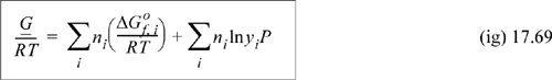
We begin the chapter with an example to provide an overview of some of the methods developed in the chapter. We have selected an introductory reaction where all species are approximated as ideal gases. For ideal gases, we show in upcoming sections that the relation between equilibrium constraint and partial pressure is written

where the symbol Π designates a product (analogous to the symbol ∑ representing the summation sign), yiP is the partial pressure (always expressed in bar) of the ith component, and vi is the stoichiometric coefficient discussed in Section 3.6. Since stoichiometric coefficients are negative for reactants, the product symbol results in a ratio of products over reactants. The solution primarily requires a mass balance relating the partial pressure to the reaction coordinate (also discussed in Section 3.6). The major steps to solving an equilibrium problem are as follows.
1. Ascertain how many phases are present and the method to be used for the equilibrium calculations. Our initial examples will use only a gas phase and determine equilibrium compositions using an equilibrium constant method. Later we will show how to use liquid and solid phases and how to use the Gibbs energy directly.
2. Use standard state properties to obtain the value of the equilibrium constant at the reaction temperature, or for the Gibbs minimization method find the Gibbs energies of the species. Usually this consists of two substeps:
a. Perform a calculation using the standard state Gibbs energies at a reference temperature and pressure.
b. Correct the temperature (and pressure for Gibbs method) to the reaction conditions.
3. Perform a material balance on the reactant and product species and relate the composition to the equilibrium constant or standard state properties from steps (1) and (2).
4. Solve for the equilibrium compositions.
The steps are made clearer by a series of examples. Steps (1) and (2) are lengthy, and the applications are easier to see by first studying steps (3) and (4) as we show in the next example. This example will help to provide motivation for understanding how to use the standard state Gibbs energies in steps (1) and (2).
Example 17.1. Computing the reaction coordinate
CO and H2 are fed to a reactor in a ratio of 2:1 at 500 K and 20 bar, where the equilibrium constant is Ka = 0.00581. (We will illustrate how to calculate Ka in Section 17.7.)
Compute the equilibrium conversion of CO.
Solution
In the expression for Ka we insert each yi P with the appropriate exponent and then insert the numerical value of pressure:

To relate the composition to the mass balance, we select a basis and use the reaction coordinate. Basis: 2 mole CO fed. Note the excess CO at the feed conditions. The reaction coordinate and method of selecting a basis have already been introduced in Section 3.6. The stoichiometry table becomes
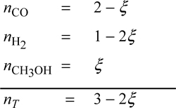
Note that all n values must stay positive, constraining the range for a physically acceptable solution to be 0 ≤ ζ ≤ 0.5. The mole fractions can be written in terms of ζ using the stoichiometry table.
Substituting the mole fractions into the equilibrium constant expression,

A trial-and-error solution is much more robust by using the difference of Eqn. 17.5 rather than the ratio of Eqn. 17.4. We solve by trial and error and substitute to get ζ recalling 0 ≤ ζ ≤ 0.5. A summary of guesses:
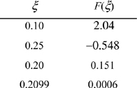
At reaction equilibrium for the given feed conditions, equilibrium is represented by ζ = 0.21. Now Eqn. 17.3 may be used to find the y’s. The conversion of CO is 0.21/2·100% = 10.5%; conversion of H2 is 2(0.21)/1·100% = 42%. Note the conversion is species-dependent with nonstoichiometric feed. Conversion can be increased further by increasing the pressure further, or by changing T where Ka is larger, provided a catalyst is available and kinetics are adequate at that T.
This example demonstrates the method to use Ka to calculate the reaction coordinate. Readers should note that the value of Ka is fixed at a given temperature, but the equilibrium value of ζ may vary for different feed conditions and often pressure for gas phase reactions as we will show in other examples. To relate the equilibrium conditions to reaction engineering textbooks, we note that most reaction engineering textbooks use conversion rather than reaction coordinate to track reaction progress. By convention, conversion is tracked for the limiting species (the species used up first at the value of ζ closest to zero in the direction of the reaction). A relation is shown in the footnote of Section 3.6.
Several other concepts are important for a general understanding of calculating reaction equilibria. First, we must understand: fundamental relations between the Gibbs energies, activities, and the equilibrium constant (Sections 17.2–17.4); simplifications that are applied for ideal gases and the effect of pressure and inerts (Section 17.5); and calculations of the temperature dependence of the equilibrium constants (Sections 17.7–17.9). Later sections illustrate the adaptation of the fundamental equations to broader applications like multiple reactions with simultaneous phase equilibria.
17.2. Reaction Equilibrium Constraint
Several sub-steps are involved in the procedure outlined in Section 17.1 steps (1) and (2) to find the equilibrium constant. In this section, we derive the equilibrium constraint, and then show how the thermodynamic properties are used to simplify to Eqn. 17.1. At reaction equilibria, the total Gibbs energy is minimized. If the composition of a system is changing, the change in the Gibbs energy is given by:
The fact that species are being created or consumed by a reaction does not alter this equation. At constant temperature and pressure, the first two terms on the right-hand side drop out:1
Substituting the definition of reaction coordinate from Eqn. 3.39,
Because G is minimized at equilibrium at fixed T and P, the derivative with respect to reaction coordinate is zero:
Now there is one unknown, ζ, in terms of which we can determine the changes in moles for all of the components. We make a further manipulation before we apply the equilibrium constraint. In phase equilibria, we found fugacity to be a convenient property to use because it simplified to the partial pressure for a component in an ideal gas mixture. We can rewrite Eqn. 17.9 in terms of fugacities. We recall our definition of fugacity dG = RT dln f. Integrating from the standard state to the mixture state of interest (cf. generalizing Eqn. 10.48),

where Gio is the standard state Gibbs energy of species i and fio is the standard state fugacity. A standard state is introduced for liquids in Section 11.3, and now we generalize the approach. The standard state is at the reaction temperature, but a specified composition (often pure) and pressure P°. Substitution of Eqn. 17.10 into Eqn. 17.9,
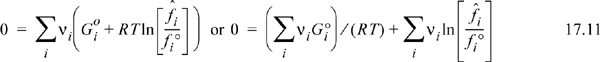
or
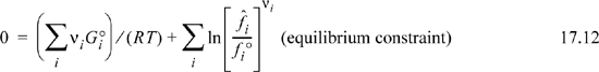
We will need to calculate both summations appearing in Eqn. 17.12, and then combine the results. Qualitatively, this equation indicates how atoms should be arranged within molecules to minimize Gibbs energy. The connection between Eqn. 17.12 and Eqn. 17.1 will become obvious as we move through the next sections. Let us work on the two summations separately. We will show that the second summation is related to the product of partial pressures for gas phase species which we define as the equilibrium constant. The first summation will relate to the negative numerical value of the equilibrium constant because the two terms of Eqn. 17.12 are equal and opposite.
17.3. The Equilibrium Constant
We now focus on the second summation of Eqn. 17.12. The ratio appearing in the logarithm is known as the activity, (cf. Eqns. 11.23 for a liquid, but now in a general sense):

The numerator ![]() represents a mixture property that changes with composition. We have developed methods to calculate
represents a mixture property that changes with composition. We have developed methods to calculate ![]() in Eqns. 10.61 (ideal gases), 10.68 (ideal solutions), 11.14 (real solution using γi), Eqn. 15.13 (real gases using
in Eqns. 10.61 (ideal gases), 10.68 (ideal solutions), 11.14 (real solution using γi), Eqn. 15.13 (real gases using ![]() ). The denominator represents the component at a specific standard state, which includes specification of a fixed composition (which can be pure or a mixture state).
). The denominator represents the component at a specific standard state, which includes specification of a fixed composition (which can be pure or a mixture state).
The second sum of Eqn. 17.12 can be manipulated after inserting the activity notation,

In a reacting mixture ![]() and/or ai will change as the reacting composition moves toward equilibrium. However, at equilibrium, the product term of activities is extremely important. We define the product term at equilibrium as the equilibrium constant Ka with the a subscript to denote that activity is used:
and/or ai will change as the reacting composition moves toward equilibrium. However, at equilibrium, the product term of activities is extremely important. We define the product term at equilibrium as the equilibrium constant Ka with the a subscript to denote that activity is used:
Combining the definition of the equilibrium constant with Eqn. 17.12, the first summation can be used to find the value of the constant:
Note that use of the term constant can be misleading because it depends on temperature. It is constant with respect to feed composition and changing mole numbers of reacting species as we will show below. We use a subscript a on the equilibrium constant to stress that it depends on activities. As we show later, there are other approximations for the equilibrium constant, and subscripts are used to differentiate between different conventions.
The Equilibrium Constant for Ideal Gases
The activity is a general property defined by Eqn. 17.13. We have seen it applied to liquids in Section 11.5. For ideal gases, the numerator of the activity is ![]() . We complete the formula for activity by selecting the standard state. For gaseous reacting species, the convention is to use a standard state of the pure gas at P° = 1 bar. For an ideal gas, fio = Po (Eqn. 9.29). Thus, fio = 1 bar. The fugacity ratio (activity) is dimensionless provided that we always express the partial pressure in bar. The second sum of Eqn. 17.12 for ideal gases simplifies to
. We complete the formula for activity by selecting the standard state. For gaseous reacting species, the convention is to use a standard state of the pure gas at P° = 1 bar. For an ideal gas, fio = Po (Eqn. 9.29). Thus, fio = 1 bar. The fugacity ratio (activity) is dimensionless provided that we always express the partial pressure in bar. The second sum of Eqn. 17.12 for ideal gases simplifies to

where the first two equalities are general, but the last is restricted to ideal gases. We will later reevaluate the fugacity ratio for nonideal gases, liquids, and solids. Now let us examine the first sum of Eqn. 17.12 which will give us the value of Ka.
17.4. The Standard State Gibbs Energy of Reaction
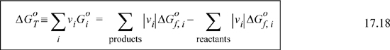
The first term on the right side of Eqns. 17.12 and 17.16, ![]() , is called the standard state Gibbs energy of reaction at the temperature of the reaction, which we will denote
, is called the standard state Gibbs energy of reaction at the temperature of the reaction, which we will denote ![]() . The standard state Gibbs energy of reaction is analogous to the standard state heat of reaction introduced in Section 3.6. The standard state Gibbs energy for reaction can be calculated using Gibbs energies of formation.
. The standard state Gibbs energy of reaction is analogous to the standard state heat of reaction introduced in Section 3.6. The standard state Gibbs energy for reaction can be calculated using Gibbs energies of formation.
As an example, for CH4(g) + H2O(g) → CO(g) + 3H2(g)
It may be helpful to think of the sum as representing a path via Hess’s law where the reactants are “unformed” to the elements and then “formed” into the products. The signs of the formation Gibbs energies of the products are positive and the signs for the reactants are negative. Thus,

The Gibbs energies of formation are typically tabulated at 298.15 K and 1 bar, and special calculations must be performed to calculate ![]() at other temperatures—the calculations will be covered in Section 17.7. Like the enthalpy of formation, the Gibbs energy of formation is taken as zero for elements that naturally exist as molecules at 298.15 K and 1 bar, and the same cautions about the state of aggregation apply. Gibbs energies of formation are tabulated for many compounds in Appendix E at 298.15 K and 1 bar. Note that for water, the difference between
at other temperatures—the calculations will be covered in Section 17.7. Like the enthalpy of formation, the Gibbs energy of formation is taken as zero for elements that naturally exist as molecules at 298.15 K and 1 bar, and the same cautions about the state of aggregation apply. Gibbs energies of formation are tabulated for many compounds in Appendix E at 298.15 K and 1 bar. Note that for water, the difference between ![]() and
and ![]() is the Gibbs energy of vaporization at 298 K. The difference is nonzero because liquid is more stable. (Which phase will have a lower Gibbs energy of formation at 298.15 K and 1 bar?)
is the Gibbs energy of vaporization at 298 K. The difference is nonzero because liquid is more stable. (Which phase will have a lower Gibbs energy of formation at 298.15 K and 1 bar?)
The standard state Gibbs energy of reaction is related to the equilibrium constant through Eqn. 17.16,

Once the value of the equilibrium constant is known, equilibrium compositions can be determined, as shown in Example 17.1. The next example illustrates calculation of the Gibbs energy of reaction and the equilibrium constant.
Example 17.2. Calculation of standard state Gibbs energy of reaction
Butadiene is prepared by the gas phase catalytic dehydrogenation of 1-butene:
Calculate the standard state Gibbs energy of reaction and the equilibrium constant at 298.15 K.
Solution
We find values tabulated for the standard state enthalpies of formation and standard state Gibbs energy of formation at 298.15 K.

The equilibrium constant is determined from Eqn. 17.16;

This reaction is not favorable at room temperature because the equilibrium constant is small.
Composition and Pressure Independence of Ka
The use of standard states for calculating ![]() has important implications on the composition and pressure independence of Ka. The standard state is at a fixed pressure, P°. Thus,
has important implications on the composition and pressure independence of Ka. The standard state is at a fixed pressure, P°. Thus, ![]() is independent of pressure. The standard states are also at fixed composition (often pure), and thus
is independent of pressure. The standard states are also at fixed composition (often pure), and thus ![]() is independent of equilibrium composition. Looking at Eqn. 17.20, we conclude that because
is independent of equilibrium composition. Looking at Eqn. 17.20, we conclude that because ![]() is independent of equilibrium composition and pressure, Ka is independent of equilibrium composition and pressure. One important point is that the state of aggregation in the standard state is important and the values of
is independent of equilibrium composition and pressure, Ka is independent of equilibrium composition and pressure. One important point is that the state of aggregation in the standard state is important and the values of ![]() and Ka do depend on the state of aggregation in the standard state; this point will be clarified in later sections.
and Ka do depend on the state of aggregation in the standard state; this point will be clarified in later sections.
We have now demonstrated steps 2(a), 3, and 4 for the procedure given in Section 17.1. The concepts have been demonstrated, but we must correct the temperature before doing calculations at temperatures other than 298.15 K. The butadiene reaction of Example 17.2 becomes more favorable with a larger Ka at higher temperatures. We will discuss some important aspects of the effects of pressure and inerts and also discuss reaction spontaneity before showing the calculation of temperature corrections.
17.5. Effects of Pressure, Inerts, and Feed Ratios
At a given temperature, equilibrium values of the reaction coordinate are affected by pressure, inerts, and feed ratios. The principle that changing the quantities affects equilibrium conversions is known as Le Châtelier’s principle in honor of Henry Louis Le Châtelier who first characterized the phenomenon. An understanding of Le Châtelier’s principle is important for operating industrial reactions. Two important modifications led to significant hydrogen conversions in Example 17.1 even though the equilibrium constant was small—use of pressure and nonstoichiometric feed.
Henry Louis Le Châtelier (1850–1936) was a French chemist. He was elected to the French Académie des Sciences and the Royal Swedish Academy of Sciences in 1907.
Pressure Effects
Pressure has little effect on the activities of condensed species (e.g., the Poynting correction is typically small) and thus it has a primary significance only for reactions with gas phase components. Pressure has important effects when both 1) gas species are involved in reactions and 2) the stoichiometric numbers of gas species are different for reactants and products. When the stoichiometric moles of gas species are the same for reactants and products, P has no effect by the ideal gas approximation, and for nonideal gases only indirect effects due to fugacity coefficients.
The equilibrium constants for ideal gases can be written
This form makes the pressure effect more obvious. As mentioned above, when the stoichiometric number of gas moles is the same for products and reactants, Σvi = 0 and the pressure effect drops out. When the stoichiometric numbers of vapor reactant moles is greater than the stoichiometric numbers of product vapor moles, an increase in pressure will drive the reaction to higher conversions,. Σvi < 0. When the stoichiometric gas mole ratios are reversed, a decrease in pressure will help drive the reaction to higher conversions, Σvi > 0. In Example 17.1 the pressure of 20 bar was important to yield significant conversions. It can be helpful to consider that qualitatively the pressure “squeezes” the reaction towards the side with fewer gas moles. As an exercise, determine the reaction coordinate for the same feed when the pressure is 1 bar.
Inerts
A component that does not participate in a reaction is called inert. Inert gas components often have an indirect, but important effect on the equilibrium reaction coordinate when gas phase species are present. Inerts change the overall mole fractions and thus mitigate the pressure effects. When Σvi > 0, adding an inert will increase conversion at a fixed total pressure. However, when Σvi < 0, the mitigation of the pressure effect is undesirable and inerts should be avoided. Qualitatively, the presence of an inert decreases the “squeezing” effect mentioned above.
Nonstoichiometric Feed
Conversions of specific reactants are influenced using nonstoichiometric feed. In Example 17.1, excess CO was fed to the reactor; conversions were 42% (H2), and 10.5% (CO). Generally, an excess of one reactant will tend to increase conversion of the other reactant. The effect can be seen qualitatively using Eqn. 17.2. For a given Ka, at a certain value of yCH3OH, a higher value of yCO results in a lower value of yH2. When using stoichiometric feed (CO:H2 = 1:2) in Example 17.1, the equilibrium conversions of H2 and CO are equal (40.6%). Example 17.1 includes both excess CO and a pressure effect. The excess CO in Example 17.1 is high enough to mitigate the beneficial pressure effect in a manner similar to an inert gas. The feed ratio giving highest H2 conversion for the specified conditions uses less excess CO, (CO:H2 = 1:1), which results in conversions of 45.2% (H2) and 22.6% (CO). Use of nonstoichiometric feed is common in industrial reactions because in some cases it helps avoid side reactions in addition to effects on equilibrium.
Example 17.3. Butadiene production in the presence of inerts
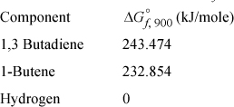
Consider again the butadiene reaction of Example 17.2 on page 648. Butadiene is prepared by the gas phase catalytic dehydrogenation of 1-butene, at 900 K and 1 bar.
a. In order to suppress side reactions, the butene is diluted with steam before it passes into the reactor. Estimate the conversion of 1-butene for a feed consisting of 10 moles of steam per mole of 1-butene.
b. Find the conversion if the inerts were absent and side reactions are ignored.
c. Find the total pressure that would be required to obtain the same conversion as in (a) if no inerts were present.
In the earlier example, we determined the value at 298.15 K for ![]() . Now we need a value at 900 K. The next section explains how the value at 900 K may be obtained. For now, use the following data for
. Now we need a value at 900 K. The next section explains how the value at 900 K may be obtained. For now, use the following data for ![]() at 900 K and 1 bar:
at 900 K and 1 bar:
Solution

a. Basis of 1 mole 1-butene feed. Set up reaction coordinate, using I to indicate inerts,.

The physical range of the solution is 0 ≤ ξ ≤ 1. P = 1 bar ⇒ 1.242 ξ2 + 2.42 ξ – 2.662 = 0 ⇒ ξ = 0.784. For the basis of 1 mol 1-butene feed, the conversion is 78.4%.
b. nI = 0 and the basis of feed is the same and 0 ≤ ξ ≤ 1. The total number of moles is nT = 1 + ξ; 1.242ξ2 – 0.242 = 0; ξ = 0.44, so conversion decreases to 44% without inert.
c. Rearranging the equilibrium expression for pressure, P–1 = ξ2 / [0.242 · (1 – ξ) · (1 + ξ)], 0 ≤ ξ ≤ 1.
Inserting a reaction coordinate of ξ = 0.784 gives P = 0.152 bar. So the reaction would need to run at a much lower pressure without the inerts to achieve the same conversion. In other words, inerts serve to dilute the fugacities of the products and suppress the reverse reaction since there are more moles of product than reactant.
17.6. Determining the Spontaneity of Reactions
In our preliminary examples, we have assumed rather idealized cases where none of the products are present in the inlet. However, in some cases, products may be present and then the reaction direction may not be as we anticipate. We can look at the reaction thermodynamics in a slightly different way to determine the direction of the reaction under given compositions, T and P. Starting from Eqn. 17.10, we may add by weighting with the stoichiometric numbers, resulting in

The term ![]() on the left side is called the Gibbs energy of reaction and is given the symbol ΔGT. Note that this is a different term than the standard state Gibbs energy of reaction (the second term) that uses the superscript °. Thus, we can write,
on the left side is called the Gibbs energy of reaction and is given the symbol ΔGT. Note that this is a different term than the standard state Gibbs energy of reaction (the second term) that uses the superscript °. Thus, we can write,

A reaction with ![]() is called exergonic and results in Ka > 1, and a reaction with
is called exergonic and results in Ka > 1, and a reaction with ![]() is called endergonic, resulting in Ka < 1. This provides an indication of whether the equilibrium favors products or reactants, but does not mean that reactions with small values of Ka cannot be conducted industrially. For example, Example 17.1 involved a small Ka (thus endergonic with
is called endergonic, resulting in Ka < 1. This provides an indication of whether the equilibrium favors products or reactants, but does not mean that reactions with small values of Ka cannot be conducted industrially. For example, Example 17.1 involved a small Ka (thus endergonic with ![]() ), yet the conversion of H2 was 42%. The propensity for the reaction to go forward or backward depends instead on the Gibbs energy of reaction ΔGT at the concentrations represented by the fugacity ratios. If the conditions provide ΔGT < 0, then the Gibbs energy is lowered when the reaction proceeds in the forward direction. If we evaluate conditions and ΔGT > 0, then the reaction goes in the reverse direction than what we have written. In either case, the concentrations adjust until the system reaches the equilibrium condition, ΔGT = 0, and then Eqn. 17.12 applies. In summary, the direction a reaction proceeds is determined by ΔGT, not by
), yet the conversion of H2 was 42%. The propensity for the reaction to go forward or backward depends instead on the Gibbs energy of reaction ΔGT at the concentrations represented by the fugacity ratios. If the conditions provide ΔGT < 0, then the Gibbs energy is lowered when the reaction proceeds in the forward direction. If we evaluate conditions and ΔGT > 0, then the reaction goes in the reverse direction than what we have written. In either case, the concentrations adjust until the system reaches the equilibrium condition, ΔGT = 0, and then Eqn. 17.12 applies. In summary, the direction a reaction proceeds is determined by ΔGT, not by ![]() . Note when evaluating the fugacity term for determining spontaneity that the actual conditions are used, not the equilibrium conditions. At the feed conditions of Example 17.1, yCH3OH = 0, which ensures ΔGT < 0 at the feed conditions even though
. Note when evaluating the fugacity term for determining spontaneity that the actual conditions are used, not the equilibrium conditions. At the feed conditions of Example 17.1, yCH3OH = 0, which ensures ΔGT < 0 at the feed conditions even though ![]() .
.
![]() The propensity for a reaction to go forward or backward under actual conditions is determined by ΔGT, not
The propensity for a reaction to go forward or backward under actual conditions is determined by ΔGT, not ![]() .
.
17.7. Temperature Dependence of Ka
Always remember that ![]() depends on the standard state, which changes with temperature. Comparing Examples 17.2 and 17.3,
depends on the standard state, which changes with temperature. Comparing Examples 17.2 and 17.3, ![]() at 298 K (Ka = 1E-14), but decreases to
at 298 K (Ka = 1E-14), but decreases to ![]() at 900 K (Ka = 0.242). In order to calculate
at 900 K (Ka = 0.242). In order to calculate ![]() , it may seem that we need to know ΔGfo for each compound at all temperatures. Fortunately this is not necessary because the
, it may seem that we need to know ΔGfo for each compound at all temperatures. Fortunately this is not necessary because the ![]() can be determined from the Gibbs energy for the reaction at a certain reference temperature (usually 298.15 K) together with the enthalpy for the reaction and the heat capacities of the species.
can be determined from the Gibbs energy for the reaction at a certain reference temperature (usually 298.15 K) together with the enthalpy for the reaction and the heat capacities of the species.
Suppose we have a table of standard energies of formation at 298.15 K but we would like the value for ![]() at some other temperature. We can account for temperature effects by applying classical thermodynamics to the change in Gibbs energy with respect to temperature using the Gibbs-Helmholtz relation,
at some other temperature. We can account for temperature effects by applying classical thermodynamics to the change in Gibbs energy with respect to temperature using the Gibbs-Helmholtz relation,
which results in the van’t Hoff equation:


For accurate calculations, we must recognize that the heat of reaction depends on temperature. We have developed the standard heat of reaction in Section 3.6 and discussed the temperature dependence there. We show later that an assumption of a temperature-independent heat of reaction results in a short-cut approximation that is often close to the full calculation. We first show the full calculation. Substituting into the van’t Hoff equation (Eqn. 17.26) and integrating again,
where we previously described finding J in Eqn. 3.46 on page 113. If desired, all values at TR can be lumped together in a constant, I.
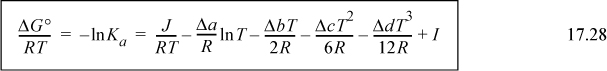
The constant I may be evaluated from a knowledge of ΔGo298 by plugging in T = 298.15 on the right-hand side as illustrated below.
Example 17.4. Equilibrium constant as a function of temperature
The heat capacities of ethanol, ethylene, and water can be expressed as CP = a + bT + cT2 + dT3 where values for a, b, c, and d are given below along with standard energies of formation. Calculate the equilibrium constant ![]() for the vapor phase hydration of ethylene at 145°C and 320°C.
for the vapor phase hydration of ethylene at 145°C and 320°C.

Solution

Taking 298.15 K as the reference temperature,
The variable J may be found with Eqn. 3.46 on page 113 at 298.15 K.
ΔH298.15o = –45,625 = J + ΔaT + (Δb/2)·T2 + (Δc/3)·T3 + (Δd/4)T4 = J + (9.014 – 3.806 – 32.24) T + [(0.2141 – 0.1566 – 0.0019)/2] T2 + [(–8.39 + 8.348 – 1.055)(1E-5)/3] T3 + [(1.373 –17.55 + 3.596)(1E-9)/4] T4
= J – 27.032 T + 0.02779 T2 – (3.657E-6)T3 – (3.145E-9)T4
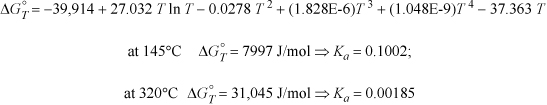
Plugging in T = 298.15 K, and solving for J, J = –39.914 kJ/mole. Using this result in Eqn. 17.28 at 298.15 K will yield the variable I.
ΔGTo/RT = –39,914/(8.314·T) + 27.032/8.314 ln T – [(5.558E-2)/(2·8.314)] T +[(1.097E-5)/(6·8.314)]T2 + [(1.258E-8)/(12·8.314)]T3 + I
Plugging in ΔGRo at 298.15K, ΔGTo/RT = –7546/8.314/298.15 = 3.0442. Plugging in for T on the right-hand side results in I = –4.494.
The resultant formula to calculate ![]() at any temperature is
at any temperature is
17.8. Shortcut Estimation of Temperature Effects
Recall Eqn. 17.25, which we refer to as the general van’t Hoff equation:
We can make rapid estimates of the equilibrium constant when we make the approximation that ΔHTo is independent of temperature. That is, suppose ΔCP = Δa = Δb = Δc = Δd = 0, which means the sensible heat effects for the reactants and products are the same. This is most closely approximated when all species are about the same molecular size and the same state of aggregation. With this approximation, ![]() in Eqn. 17.27, or we can integrate Eqn. 17.25 directly to obtain what we refer to as the shortcut van’t Hoff equation:
in Eqn. 17.27, or we can integrate Eqn. 17.25 directly to obtain what we refer to as the shortcut van’t Hoff equation:
This equation enables rapid screening for the effects of temperature and the detailed van’t Hoff can be used as a follow-up calculation. As a particular observation, we take special note from the above equation that exothermic reactions (ΔHT < 0) lead to Ka decreasing as temperature increases, and endothermic reactions (ΔHT > 0) lead to Ka increasing as temperature increases. This means that equilibrium conversion (for a specified feed) decreases with increasing temperature for exothermic reactions, and increases for endothermic reactions. This effect is illustrated in Fig. 17.1. The emphasis is placed on equilibrium because reaction rates increase with temperature. Industrial application of exothermic reactions are almost always run at elevated temperatures even though the equilibrium constant decreases at high temperature. For all reactions, the reaction rate will approach zero as equilibrium is approached. The benefit of faster kinetics typically outweighs the smaller equilibrium constant for exothermic reactions when economics are considered. There connection between equilibrium constants and kinetic rates that approach zero is explained in Section 17.15.
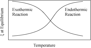
Figure 17.1. Qualitative behavior of equilibrium conversion for exothermic and endothermic reactions.
The approximate results of the shortcut van’t Hoff equation should be followed with the detailed van’t Hoff for critical applications. To improve shortcut estimates, the detailed van’t Hoff can be used at Tnear within 100 K of the temperatures of interest to calculate ΔGTnearo and ΔHTnearo. Then the values at Tnear can be used as the reference values in Eqn. 17.29.
Example 17.5. Application of the shortcut van’t Hoff equation
Apply the shortcut approximation to the vapor phase hydration of ethylene. This reaction has been studied in the previous example, and the Gibbs energy of reaction and heat of reaction can be obtained from that example.
Solution

The results are very similar to the answer obtained by the general van’t Hoff equation in Example 17.4.
17.9. Visualizing Multiple Equilibrium Constants
Plots of equilibrium constants provide a rapid method to visualize the gross trends and orders of magnitude. Fig. 17.2 illustrates how several reactions can be illustrated in a single graph. The equilibrium constants are calculated with the full temperature dependence. Note that the plots are nearly linear as would be approximated by the short-cut van’t Hoff. Exothermic reactions have a negative slope and endothermic reactions have a positive slope. When dealing frequently with a set of reactions, such a graph can serve as a “road map” where the optimal temperature window of operation maximizes desired products while minimizing by-products and potential coupling of reactions.

Figure 17.2. Graphical analysis of competing reactions.
The reactions of Fig. 17.2 are typically involved in many high-profile applications including: combustion, chemical-vapor infiltration, reforming, coking during reforming, space station gas management, electrolysis, and the hydrogen economy. Several of these reactions have common names which are listed below.
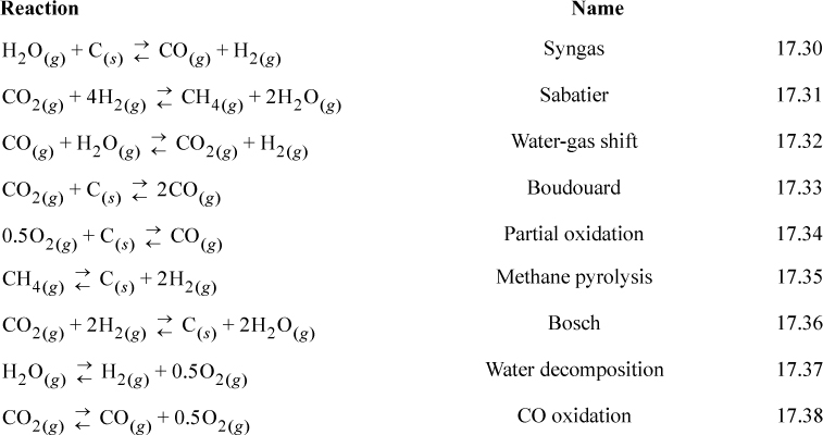
To illustrate interpretation of the graph, consider an application of the above reactions to material management in space station gas management, where an objective is to remove CO2 and provide O2. There are many ways that the reactions could be combined. On a space station sunlight is relatively abundant. Therefore, high temperatures and solar cells are available, but food must be imported. Note that the Sabatier reaction would convert waste CO2 to fuel but requires H2. Fig. 17.2 shows that the equilibrium constant is favorable below 900 K. The Bosch reaction also favors products at temperatures below 900 K. The Bosch reaction produces graphitic carbon, which can be collected in dense form and conveniently disposed. The hydrogen required for the Bosch reaction could be generated by water decomposition, which could be achieved with electrolysis or pyrolysis, with the benefit of co-producing oxygen for respiration. A small extrapolation of Fig. 17.2 shows that water pyrolysis is favorable above 2300 K.2 Coupling the Sabatier reaction with methane pyrolysis has been suggested. Methane pyrolysis is favorable above 700 K. This would produce hydrogen for other use. Hydrogen production could also be achieved by the syngas reaction, if graphitic carbon was available. H2 could be enhanced and CO removed by the water-gas shift. Catalysts can selectively alter the kinetics to minimize undesired products, although they cannot alter the equilibrium constraints. Nevertheless, all combinations are constrained by material balances, which dictate the overall reactions.
This kind of reaction network analysis is typical of many applications. For example, some simple economic considerations show why producing hydrogen by steam reforming of methane (natural gas) is the preferred method compared to electrolysis. The energetic cost of water electrolysis raises serious doubts about electrolysis feasibility on Earth. With abundant electrical energy, it might be more appropriate to operate electric vehicles. It is not practical to articulate all the ways that this kind of network analysis can be applied to modern problems, but these illustrations should suggest the manner of proceeding for many such analyses. Noting that energies of reaction are an implicit part of the analysis, a tremendous wealth of information is implied by a single graph like Fig. 17.2. Later, in Section 17.11, we demonstrate how combining an unfavorable reaction with a strongly favorable reaction can help to drive the unfavorable reaction.
17.10. Solving Equilibria for Multiple Reactions
When the equilibrium state in a reacting system depends on two or more simultaneous chemical reactions, the equilibrium composition can be found by a direct extension of the methods developed for single reactions. Each reaction will have its own reaction coordinate in which the compositions can be expressed. Some of the products of one reaction may act as reactants in another reaction, but the amount of that substance can still be written in terms of the extents of the reactions. Eventually, the material balances lead us to a system of N nonlinear equations in terms of N unknowns. We illustrate a solution by hand and then demonstrate how numerical solvers can be used.
Example 17.6. Simultaneous reactions that can be solved by hand
We can occasionally come across multiple reactions which can be solved without a computer. These are generally limited to textbook problems, but provide a starting point and test case for applying the general approach. Consider the two series/parallel gas phase reactions:
The reactions are considered series reactions because C is a product of the first reaction, but a reactant in the second. They are parallel because A is a reactant in both reactions. The pressure in the reactor is 10 bar, and the feed consists of 2 moles of A and 1 mole of B. Calculate the composition of the reaction mixture if equilibrium is reached with respect to both reactions.
Solution
The material balance gives:

Note that for a physical solution, 0 ≤ ξ1 ≤ 1, 0 ≤ ξ2 ≤ ξ1 to ensure that all mole numbers are positive. This reaction network is independent of P because Σvi = 0. The equilibrium constants are
Solving the first equation for ξ1 using the quadratic equation,
Similarly, for the second reaction,
We may now solve by trial and error. The procedure is: 1) guess ξ1; 2) solve Eqn. 17.40 for ξ2; 3) solve Eqn. 17.39 for ![]() ; 4) if
; 4) if ![]() , go to step 1. The iterations are summarized below.
, go to step 1. The iterations are summarized below.

Further iteration results in no further significant change.
These equations were amenable to the quadratic formula, but in general equilibrium criteria can be more complicated. Fortunately, standard programs available that are formulated to solve numerically multiple nonlinear systems of equations, so we can concentrate on applying the program to thermodynamics instead of developing the numerical analysis. Many software packages like Mathematica, Mathcad, MATLAB, and even Excel offer the capability to solve nonlinear systems of equations. Excel provides an especially convenient basis for illustrating the methods presented here.
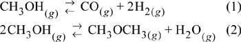
Example 17.7. Solving multireaction equilibria with Excel
Methanol has a lower vapor pressure than gasoline. That can make it difficult to start a car fueled by pure methanol. One potential solution is to convert some of the methanol to methyl ether in situ during the start-up phase of the process (i.e., automobile). At a given temperature, 1 mole of MeOH is fed to a reactor at atmospheric pressure. It is assumed that only the two reactions given below take place. Compute the extents of the two simultaneous reactions over a range of temperatures from 200°C to 300°C. Also include the equilibrium mole fractions of the various species.
Solution
A worksheet used for this solution is available in the workbook Rxns.xlsx.
Data for reaction (1) have been tabulated by Reactions Ltd.a—at 473.15 K, ΔHT = 96,865 J/mol and lnKa1,473 = 3.8205. Over the temperature range of interest we can apply the shortcut van’t Hoff equation assuming constant heat of reaction using the data at 200°C as a reference.
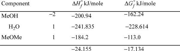
Data for reaction (2) can be obtained from Appendix E for MeOH and water. For DME, the values are from Reid et al. (1987).b
The shortcut van’t Hoff equation for this reaction gives:


Writing equations for reaction coordinates for reaction 1:
and for reaction 2:
These two equations are solved simultaneously for ξ1 and ξ2. We have rearranged the objective functions to eliminate the ratios of ξ functions and use differences instead because the Excel Solver is much more robust with this mathematical form. The solution is implemented in the worksheet DUALRXN in Rxns.xlsx or Matlab Ex17_07.m. In the example here (see Fig. 17.3), the ΔCP for both reactions is neglected. The equations derived above are entered directly into the cells, and the Solver tool is called.c You will need to designate one of the reaction equations as the target cell, the value of which is set to zero. The other reaction equation should be designated as a constraint (also set to zero). The cells with the reaction coordinates are the variables to be changed to obtain a solution. Under “options,” you may want to specify the “conjugate” method, since that generally seems to converge more robustly for the reacting systems typically encountered. Generally, the Solver tool will require a reasonably accurate initial guess to keep it from converging on absurd results (e.g., yi < 0). The initial guess can be easily developed by varying the values in the reaction-extent cells until the target cells move in the right direction. It sounds difficult, but the given worksheet will get you started, then you can experiment with initial guesses and experience how good your initial guesses need to be.
a. These data are slightly different from values calculated using tabulated properties from Appendix E, but such variations are common in thermochemical data. The equilibrium compositions are about the same if the example is reworked using data from Appendix E.
b. Reid, R., Prausnitz, J.M., Poling, B. 1987. The Properties of Gases and Liquids, 4th ed. New York: McGraw-Hill.
c. See the online supplement for an introduction to Solver.
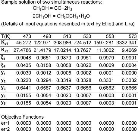
Figure 17.3. Worksheet DUALRXN from workbook Rxns.xlsx for Example 17.7 showing converged answers at several temperatures.
17.11. Driving Reactions by Chemical Coupling
Frequently, one may encounter a reaction that is not favored by Ka, and manipulation of temperature or pressure or feed composition provides only limited benefit for the desired conversion. In these cases, it may be possible to couple the reaction to another, more favorable, reaction to drive the overall production forward. Biological systems use coupling extensively. The building of sugars and biological tissue from CO2 and water is thermodynamically unfavorable. Carbon is fully oxidized and it must be reduced to create carbohydrates, and the reactions are endergonic at room temperature. These reactions are achieved by coupling an unfavorable carbon reduction with a strongly exergonic reaction.
To illustrate the principles of chemical coupling with a simple set of reactions, let us consider the production of butadiene from butene dehydrogenation at 900 K. We have investigated this reaction in Example 17.3 where we showed that the reaction is endergonic: Ka = 0.242 is small. The example showed that conversion is improved by diluting with steam. Consider instead if CO2 is fed to the reactor and a catalyst is provided for the water-gas shift reaction (c.f. Eqn. 17.32). The CO2 could then react with H2 product of the dehydrogenation, inducing higher conversion for the dehydrogenation. The hydrogen product is removed by Le Châtelier’s principle and the dehydrogenation reaction is pulled forward.
Example 17.8. Chemical coupling to induce conversion
Example 17.3(a) considered use of steam as a diluent where the conversion was found to be 78% using 10 moles of steam as diluent and only 44% without the diluent. Consider the conversion by inducing higher conversion by replacing the 10 mole steam with 10 mole CO2 which adds the water-gas shift reaction. For the water-gas shift written as ![]() , Ka2 = 0.441 at 900 K. What is the conversion of 1-butene at 900 K and 1 bar?
, Ka2 = 0.441 at 900 K. What is the conversion of 1-butene at 900 K and 1 bar?
Solution
The butadiene reaction has been written in Example 17.3(a) and ξ1 will be used for that 1-butene reaction and ξ2 will be used for the water-gas shift reaction. The stoichiometry table is,
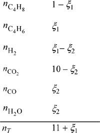
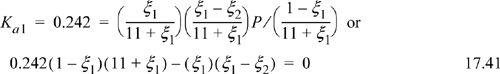
Physical limits for the reaction coordinates are 0 ≤ ξ1 ≤ 1 and 0 ≤ ξ2 ≤ ξ1. Solving Eqns. 17.41 and 17.42 simultaneously, we find ξ1 = 0.949 and ξ2 = 0.792. Reviewing previous examples, the conversion at 1 bar was only 44% without an inert, increased to 78% with an inert, and increased to 95% using CO2 to induce conversion by reaction coupling. Note that even though the water-gas shift equilibrium constant is not very large, it makes a significant difference in the conversion of 1-butene. Whether this is implemented depends on the feasibility of economically separating the products.
Chemical coupling can be classified in three ways: (1) induction, where a second reaction “pulls” a desired reaction by removing a product as in Example 17.8; (2) pumping, where the second reaction creates additional reactant for the desired reaction to “pump”; or (3) complex, where both induction and pumping are operative.3 An example of chemical pumping starts with the reaction of methyl chloride and water to form methanol and hydrochloric acid.
By adding the methyl chloride synthesis reaction,
This overall reaction becomes (adding the reactions, and take the product of the Kas):
The large equilibrium constant of 17.44 forms CH3Cl(g) readily, to pump reaction 17.43 via Le Châtelier’s principle. Through chemical coupling, the prospects of developing a feasible reaction network are virtually endless.
17.12. Energy Balances for Reactions
We have previously introduced the energy balance in Section 3.6 and also discussed adiabatic reactors. In this section we consider that there may be a there is a maximum possible value of ξ (outlet conversion) due to chemical equilibrium. Equilibrium may affect both adiabatic and nonadiabatic reactors, but we cover adiabatic reactors, and the extension to nonadiabatic should be obvious with the inclusion of the heat term.
Adiabatic Reactors
The energy balance for a steady-state adiabatic flow reactor is given in Eqn. 3.53 on page 118. The variables Tout and ![]() from the energy balance also appear in the equilibrium constraint that will govern maximum conversion. Earlier, in Chapter 3, we considered the reaction coordinate to be specified. However, in a reaction-limited adiabatic reactor, we must solve the energy balance together with the equilibrium constraint to simultaneously determine the maximum conversion and adiabatic outlet temperature. Using the energy balance from Eqn. 3.53, do the following.
from the energy balance also appear in the equilibrium constraint that will govern maximum conversion. Earlier, in Chapter 3, we considered the reaction coordinate to be specified. However, in a reaction-limited adiabatic reactor, we must solve the energy balance together with the equilibrium constraint to simultaneously determine the maximum conversion and adiabatic outlet temperature. Using the energy balance from Eqn. 3.53, do the following.
1. Write the energy balance, Eqn 3.53. Calculate the enthalpy of the inlet components at Tin.
2. Guess the outlet temperature, Tout. Calculate the enthalpy of the outlet components at Tout.
3. Determine ![]() at Tout using the chemical equilibrium constant constraint.
at Tout using the chemical equilibrium constant constraint.
4. Calculate ![]() for this conversion.
for this conversion.
5. Check the energy balance for closure.
6. If the energy balance does not close, go to step 2.
As you might expect, this type of calculation lends itself to numerical solution, such as the Solver in Excel.
Example 17.9. Adiabatic reaction in an ammonia reactor
Estimate the outlet temperature and equilibrium mole fraction of ammonia synthesized from a stoichiometric ratio of N2 and H2 fed at 400 K and reacted at 100 bar. How would these change if the pressure was 200 bar?
Solution
For a rough estimate we will use the shortcut approximation of temperature effects. Furthermore, we will assume Kϕ ≈ 1. (Is this a good approximation or not?a) Therefore we obtain,
Basis: Stoichiometric ratio in feed.
For the purposes of the example, the shortcut van’t Hoff equation will be used to iterate on the adiabatic reactor temperature. However, the full van’t Hoff method will be used to obtain ![]() and
and ![]() at an estimated nearby temperature Tnear = 600K as suggested in Section 17.8. Then the shortcut van’t Hoff equation will be used over a limited temperature range for less error. The energy balance will also use
at an estimated nearby temperature Tnear = 600K as suggested in Section 17.8. Then the shortcut van’t Hoff equation will be used over a limited temperature range for less error. The energy balance will also use ![]() ; we will create an energy balance path through Tnear = 600K rather than 298.15K. We will compare the approximate answer with the full van’t Hoff method at the end of the example.
; we will create an energy balance path through Tnear = 600K rather than 298.15K. We will compare the approximate answer with the full van’t Hoff method at the end of the example.
For ammonia, ![]() ,
, ![]() . Since the reactants are in the pure state, the respective reactant formation values are zero, and therefore the formation values for ammonia represent the standard state values for the reaction. Inserting the formation values along with the heat capacities into the detailed van’t Hoff equation—one of the Ka calculators highlighted in the margin note to Example 17.4 on page 653 is used—at an assumed temperature of 600 K, the values obtained are
. Since the reactants are in the pure state, the respective reactant formation values are zero, and therefore the formation values for ammonia represent the standard state values for the reaction. Inserting the formation values along with the heat capacities into the detailed van’t Hoff equation—one of the Ka calculators highlighted in the margin note to Example 17.4 on page 653 is used—at an assumed temperature of 600 K, the values obtained are ![]() and Ka,600 = 0.0417659. Then the shortcut van’t Hoff in the vicinity will be
and Ka,600 = 0.0417659. Then the shortcut van’t Hoff in the vicinity will be
From an assumed value of T, this equation will provide the equilibrium constant. Some manipulation is necessary to obtain the material balance from Ka,T. Plugging the mole fraction expressions into Eqn. 17.17, and collecting the fractions 1/2 and 3/2,
defining ![]()
Applying the quadratic formula,
The strategy will be to guess T, and calculate Ka,T, M, and ![]() .
. ![]() will be used in Eqn. 17.46 to perform the material balance. The material balance will be combined with the energy balance using the Heat of Reaction method (cf. Example 3.6), until the energy balance closes as represented by:
will be used in Eqn. 17.46 to perform the material balance. The material balance will be combined with the energy balance using the Heat of Reaction method (cf. Example 3.6), until the energy balance closes as represented by:

Heat capacity integrals and the energy balance have been entered in the workbook Rxns.xlsx. At the initial guess of 600 K, the F(T) of Eqn. 17.49 is 19.4 kJ. A converged result is found at 699 K shown in Fig. 17.4 and the ![]() = 0.33, conversion of feed is 33%. At 200 bar, the answer is 739 K, and conversion is 38%.
= 0.33, conversion of feed is 33%. At 200 bar, the answer is 739 K, and conversion is 38%.

Figure 17.4. Display from Rxns.xlsx showing a converged answer.
The detailed van’t Hoff is available in the same workbook and results in 698 K and 33% conversion at 100 bar, and 737 K and 37% conversion at 200 bar.
a. We can evaluate this assumption by calculating the reduced temperatures at the end of our calculation and estimating the virial coefficients, then fugacity coefficients.
Graphical Visualization of the Energy Balance
The energy balance is presented in Fig. 3.6 on page 119. The difference here is that the appropriate curve from Fig. 3.6 is superimposed on the plot and the outlet conversion and outlet temperature are determined by the intersection of the energy balance line and the equilibrium line. Fig. 17.5 illustrates an exothermic reaction. In the event that the reaction does not reach equilibrium because of kinetic limitations, the reaction coordinate must be located along the energy balance line below the equilibrium value. For the case of the ammonia reaction, the equilibrium constraint curve could be generated by inserting various temperatures in Eqn. 17.47 and then determining the reaction coordinate from Eqn. 17.48. The energy balance is plotted using Eqn. 3.55. The dot in the figure represents the point where the energy balance and equilibrium constraint are both satisfied. Note that an endothermic reaction will have an energy balance with a negative slope, and the equilibrium line will change shape as shown in Fig. 3.6, making the plot for an endothermic reaction a mirror image of Fig. 17.5 reflected across a vertical line at Tin.

Figure 17.5. Approximate energy balance for an exothermic reaction. The dot simultaneously represents the equilibrium outlet conversion and reaction coordinate value at the adiabatic outlet temperature. The plot for an endothermic reaction will be a mirror image of this figure as explained in the text.
17.13. Liquid Components in Reactions
When a liquid component is involved in a reaction, the fugacity ratio for activity in Eqn. 17.15 is typically expressed using activity coefficients. Thus,

where P is expressed in bar, and the Poynting correction is often negligible, as shown. Another important change in working with liquid components is that in determining Ka liquid phase values are used for ![]() , not the ideal gas values. Frequently these values are not available in the literature, so it is common to express equilibrium in terms of temperature-dependent correlations for Ka as described in Section 17.18.
, not the ideal gas values. Frequently these values are not available in the literature, so it is common to express equilibrium in terms of temperature-dependent correlations for Ka as described in Section 17.18.
Equilibrium constants calculated using liquid phase species are different from the equilibrium constants for the same reactants and products in the gas phase. Consider that ![]() for the vapor phase. If a vapor phase reaction is simultaneously in phase equilibrium with a liquid phase with the same components, by modified Raoult’s law we could replace
for the vapor phase. If a vapor phase reaction is simultaneously in phase equilibrium with a liquid phase with the same components, by modified Raoult’s law we could replace ![]() . However, for the liquid equilibrium constant we should use only the activity (Eqn. 17.50) without the vapor pressure. Thus, we conclude that the equilibrium constants for the liquid phase reaction must be different from the equilibrium constant for the same vapor phase reaction, and also that the standard state Gibbs energy change for the same reaction must be different.
. However, for the liquid equilibrium constant we should use only the activity (Eqn. 17.50) without the vapor pressure. Thus, we conclude that the equilibrium constants for the liquid phase reaction must be different from the equilibrium constant for the same vapor phase reaction, and also that the standard state Gibbs energy change for the same reaction must be different.
Example 17.10. Oligomerization of lactic acid
Lactic acid is a bio-derived chemical intermediate produced in dilute solution by fermentation. Lactic acid is an α-hydroxy carboxylic acid. As an aqueous solution of lactic acid is concentrated by boiling off water, the carboxylic acid on one molecule reacts with a hydroxyl on another forming a dimer and releasing water. Denoting the “monomer” as L1 and a dimer as L2,
The dimer has a hydroxyl and carboxylic acid that can react further to form trimer L3,
As more water is removed, the chain length grows, forming oligomers. The oligomerization can be represented by a recurring reaction for chain formation. Each liquid phase reaction that adds a lactic acid molecule can be modeled with a universal temperature-independent value of Ka = 0.2023 and the solutions may be considered ideal.a Commercial lactic acid solutions are sold based on the wt% of equivalent lactic acid monomer. So 100 g of 50 wt% solution would be composed of 50 g of lactic acid monomer and 50 g of water that react to form an equilibrium distribution of oligomers. The importance of including modeling of higher oligomers increases as the concentration of lactic acid increases.
a. Determine the mole fractions and wt% of species in a 50 wt% lactic acid solution in water where the distribution is approximated by only reaction 17.51.
b. Repeat the calculations for an 80 wt% lactic acid solution in water where both reactions are necessary to approximate the distribution.
Solution
a. Basis: 100 g total, 50 g of L1 = (50 g)/(90.08 g/mol) = 0.555 mol initially, 50 g = (50 g)/(18.02 g/mol) = 2.775 mol water initially, and 3.330 mol total. The equilibrium relation is Ka = 0.2023 = xL2xH2O/(xL1)2. Since the total number of moles does not change with reaction, it cancels out of the ratio, and we can write 0.2023 = nL2nH2O/(nL1)2. Introducing reaction coordinate,
Solving, we find, ξ = 0.0193, xL1 = (0.555 – 2(0.0193))/3.33 = 0.155, xL2 = 0.0193/3.33 = 0.006, xH2O = (2.775 + 0.0193)/3.33 = 0.839. Note that although the mole fraction of L2 seems small, converting to wt%, the water content is (2.775 + 0.0193)(18.02 g/mol)/(100 g)·100% = 50.4 wt%, L1 is (0.555 – 2(0.0193))(90.08 g/mol)/(100 g)·100% = 46.5 wt%, and L2 is 0.0193(162.14 g/mol)/(100 g) · 100% = 3.1 wt%.
b. Basis: 100 g total, 80 g of L1 = (80 g)/(90.08 g/mol) = 0.888 mol initially, 20 g = (20 g)/(18.02 g/mol) = 1.110 mol water initially, and 1.998 mol total. Moles are conserved in both reactions. The equilibrium relations are Ka1 = 0.2023 = xL2xH2O/(xL1)2, Ka2 = 0.2023 = xL3xH2O/(xL2xL1). Introducing the mole numbers and reaction coordinates,
Solving simultaneously, ξ1 = 0.0907, ξ2 = 0.009, xL1 = (0.888 – 2(0.0907) – 0.009)/1.998 = 0.349, xL2 = (0.0907 – 0.009)/1.998 = 0.041, xL3 = 0.009/1.998 = 0.0045, xH2O = (1.110 + 0.0907 + 0.009)/1.998 = 0.6055. The weight fractions are: (1.110 + 0.0907 + 0.009)(18.02 g/mol)/(100 g)·100% = 21.8 wt% water, (0.888 – 2(0.0907) – 0.009)(90.08 g/mol)/(100 g)·100% = 62.8 wt% L1, and (0.0907 – 0.009)(162.14 g/mol)/(100 g)·100% = 13.2 wt% L2, 0.009(234.2 g/mol)/(100 g)·100% = 2.1 wt% L3.
a. Vu, D. T., Kolah, A.K., Asthana, N.S., Peereboom, L., Lira, C.T., Miller, D.J. 2005. “Oligomer distribution in concentrated lactic acid solutions.” Fluid Phase Equil. 236:125–135.
If a vapor state coexists with a liquid phase during a reaction, the phase equilibria and reaction equilibria are coupled. Reactions need to be considered in only one of the two phases, and the equilibrium compositions will be consistent with compositions that would have been determined by the same reaction equilibria in the other phase. Similarly, some reaction equilibria constants may be known for only one or the other of the phases, and the equilibria can be solved by using reaction equilibria for whichever phase is most convenient. Simultaneous reaction and phase equilibria can be extremely useful for driving reactions in preferred directions as we illustrate in Example 17.15.
17.14. Solid Components in Reactions
When a solid component is involved in a reaction, the fugacity ratio for activity in Eqn. 17.15 is typically expressed using activity coefficients. For a solid solution,

where P is expressed in bar, Psat represents the solid sublimation pressure, and the Poynting correction is often negligible. Commonly, multiple solids exist as physical mixtures of pure crystals as discussed in Section 14.10 on page 556. When the solids are immiscible, Eqn. 17.56 simplifies to

Similar to working with liquids, solid phase data are used for ![]() , not the ideal gas values. When these values are not available in the literature, it is common to express equilibrium in terms of temperature-dependent correlations for Ka as described in Section 17.18.
, not the ideal gas values. When these values are not available in the literature, it is common to express equilibrium in terms of temperature-dependent correlations for Ka as described in Section 17.18.
Consider the reaction:
The carbon formed in this reaction comes out as coke, a solid which is virtually pure carbon and separate from the gas phase. What is the activity of this carbon? Since it is pure, aC = 1. Would its presence in excess ever tend to push the reaction in the reverse direction? Since the activity of solid carbon is always 1 it cannot influence the extent of this reaction. How can we express these observations quantitatively? Eqn. 17.15 becomes

To compute ΔGoT as a function of temperature, we apply the usual van’t Hoff procedure. This means that CP,c can be treated just like CP of the gaseous species.
Example 17.11. Thermal decomposition of methane
A 2-liter constant-volume pressure vessel is evacuated and then filled with 0.10 moles of methane, after which the temperature of the vessel and its contents is raised to 1273 K. At this temperature the equilibrium pressure is measured to be 7.02 bar. Assuming that methane dissociates according to the reaction ![]() , compute Ka for this reaction at 1273 K from the experimental data.
, compute Ka for this reaction at 1273 K from the experimental data.
Solution
We can calculate the mole fractions of H2 and CH4 as follows. Since the temperature is high, the total number of moles finally in the vessel can be determined from the ideal gas law (assuming that the solid carbon has negligible volume): n = PV/RT = 0.702·2000/(8.314)(1273) = 0.1327. Now assume that ξ moles of CH4 reacted. Then we have the following total mass balance: nT = 0.10 + ξ. Therefore, ξ = 0.0327 and

Note that the equilibrium constant indicates that significant decomposition will occur (the reaction is exergonic, Ka > 1) and that graphite forms. Such behavior is known as “coking” and is common during industrial catalysis. Industrial application of catalysis often includes consideration of “regeneration’” of the catalyst by burning off the coke and using the heat of combustion elsewhere in the chemical plant.
17.15. Rate Perspectives in Reaction Equilibria
We have avoided discussing rate effects until now with the rationale that most coverage for reaction kinetics will occur in a course focused on reactor design. Nevertheless, there is overlap between the topics of reaction equilibria and reaction rates that can serve as a bridge between the two subjects. In all equilibrium phenomena, it is important to recognize that the balance achieved is dynamic, not static. For example, the molecules at the interface between a vapor and liquid are not stationary; they are perpetually exchanging between the vapor and liquid. Application of thermodynamics helps us understand the conditions where the balance occurs. Similarly, under conditions of chemical reaction equilibrium, the species are continuously interconverting with equal rates for the forward and reverse reactions.
From a thermodynamic perspective, the true driving force for chemical reaction is the activity. When the activities are balanced as given by Eqn. 17.15 the reaction reaches equilibrium and the forward are reverse rates are equal. The activities are directly proportional to the concentrations for liquids and vapors. Thus, it is common to use concentrations instead of activities for simple kinetic models. Consider the vapor-phase reaction,
For example, if two components, A and B, react to form C and D, then the rate of accomplishing the reaction must depend on the probability of the two components colliding with each other. This probability decreases as the concentration of one of the components diminishes. By convention the rates are typically written for the stoichiometrically limiting component. Also, they are typically written for the rate of formation per volume of reacting mixture.4 If A is the limiting reactant, the rate of the formation of A due to reaction of A with B would then be,
where the minus sign acknowledges that A is disappearing rather than forming, and the subscript f indicates reaction in the forward direction and kf is known as the forward rate constant. When the exponents on the rate equation match the stoichiometric coefficients, the reaction is called an elementary reaction. When a reaction is equilibrium-limited, it is considered kinetically reversible. Recognizing that A is formed by reaction of C and D, the reverse reaction rate for formation of A is
The net rate of formation of A must be zero at reaction equilibrium,
Recognizing that concentration of a gas phase component is related to partial pressure, [A] = yAP/RT, and similarly for other components. Rearranging Eqn. 17.63 and inserting the partial pressure results in

where in this case, Σvi = –1, but the general expression is written to help readers remember the general relation for gas phase reactions. Note the manner in which the forward and reverse reaction rate constants are related to the equilibrium constant. This means that if the forward rate constant is measured in an experiment when the product concentrations are low, then the reverse rate constant can be determined from the equilibrium constant. Note that similar relations can be written for liquid-phase elementary reactions.
Certainly many reactions have rate expression more complicated than the elementary reactions discussed here. For example, enzyme catalyzed reactions often involve a binding step that is not represented by the simple statistical concept of the elementary reaction. Many reactions involve intermediate species that must be included in the mechanism and kinetic rate law. Understanding more complex rate laws is an important skill covered in reaction engineering courses. Our intention here was to show the relation for elementary reactions and to communicate the concept of forward and reverse rates approaching each other at reaction equilibrium. Note that this means that if the reaction approaches equilibrium in the forward direction, the overall rate of disappearance of A will slow and become zero. At slow rates, the reactor volume must be large to achieve meaningful change in reaction coordinate, so it is rarely economical to run commercial reactors all the way to equilibrium. However, the calculation of the equilibrium condition is important for any reactor design in order to know the limiting conversion, and usually avoid the conditions! Often, the equilibrium constant is used to calculate the reverse rate constant from the forward rate constant as discussed above.
17.16. Entropy Generation via Reactions
When introducing entropy and reversibility in Section 4.11 on page 175, we made a general statement that spontaneous reactions generate entropy. Then, in Section 4.12 on page 177 we derived relations between availability and entropy generation. In that section, we treated a single nonreactive stream. For a reaction in a steady-state open system, Eqn. 4.54 becomes
Bout = Hout – ToSout and Bin = Hin – ToSin involve H and S evaluated at the respective Tout and Tin. Enthalpies of mixed streams were first introduced in Chapter 3 and entropies for mixed streams in Chapter 4.5 Models for departures functions and excess properties in Chapters 11–15 can be added to improve the mixture property values. The concepts for proper choice of a reference state for properties is important as discussed in Chapter 3 in the section Energy Balances for Reactions on page 113. The flow terms in Eqn. 17.65 are not the same as the Gibbs energy, but the availability will decrease with a spontaneous reaction. Therefore, both sides of the equation will be negative, and shaft work will not be obtained (a normal situation in an industrial reactor), and then entropy is generated. Note that entropy generation can be decreased for a spontaneous reaction only if work is produced. For an electrochemical redox reaction (Chapter 18), the process can produce some electrical work, which is one reason that fuel cells are of much current interest. For a closed-system process, the analysis is similar to the open-system process. The relation is seen most readily if To = T (and additional work can be obtained using a heat engine between T and To), and at constant pressure, the closed system balance (Eqn. 4.57) becomes
We conclude that production of nonexpansion/contraction work equal to changes in the Gibbs energy is necessary to eliminate entropy generation. Note that it is possible to relate the total work from a reaction to Helmholtz energy using Eqn. 4.58.
17.17. Gibbs Minimization
A remarkably simple technique can be applied to solve for the equilibrium compositions of species. It is most effective when only a gas phase is present. This technique recognizes the simplicity of the fundamental problem of minimizing the Gibbs energy at equilibrium. By expressing the total Gibbs energy of the mixture in terms of its ideal solution components, we can simply request that the value of the Gibbs energy be minimized. The Gibbs energy of the mixture is calculated by Eqn. 10.42 and the needed chemical potential (partial molar Gibbs energy) is given by Eqn. 10.59:
where the last equality assumes all components are ideal gases. If we take the reference state as the elements in their natural form at the standard state, then, at the standard state pressure, ![]() . However, frequently the reactions are not at standard state pressure. The pressure effect on Gibbs energy is given by Eqn. 9.17. When the pressure effect is added,
. However, frequently the reactions are not at standard state pressure. The pressure effect on Gibbs energy is given by Eqn. 9.17. When the pressure effect is added,

Combining Eqns. 17.67 and 17.68 results in
To find equilibrium compositions, we just need to minimize Eqn. 17.69 by varying the mole numbers ni of each component while simultaneously satisfying the atom balance. Note that the mole fractions in the equation will also change as the mole numbers are varied. We do not need to explicitly write out the reactions. This method assumes that equilibrium is reached by whatever system of reactions is necessary. Most process simulators provide Gibbs minimization as a process unit.
Example 17.12. Butadiene by Gibbs minimization
Review Example 17.3(a) where steam is used to enhance conversion for 1-butene dehydrogenation. Gibbs energies of formation at 900 K for the hydrocarbons are summarized in that example.
The Gibbs energy of formation for water at 900 K is –198.204 kJ/mol. Vary conversion by selecting values of the reaction coordinate, calculating the Gibbs energy by Eqn. 17.69, and plotting the total Gibbs energy as a function of reaction coordinate. Demonstrate that Gibbs energy is minimized. Compare the equilibrium composition with that found in Example 17.3(a).
Solution
The initial moles of feed are 1 mol of 1-butene and 10 moles of steam. As an example calculation, select ξ = 0.1. Then the material balance provides, nC4H8 = 0.9, nC4H6 = nH2 = 0.1, nH2O = 10. The mole fractions are yC4H8 = 0.9/(0.9 + 2(0.1) + 10) = 0.08108, yC4H6 = yH2 = 0.0090, yH2O = 0.9009, and inserting the quantities into Eqn. 17.69, gives (inserting components in the order given above)

Repeating the calculation at various extents of reaction results in the following plot:

Careful analysis would show that the minimum is at ξ = 0.784 as in the earlier example. Note the changes in values are a small percentage of the absolute values of the total Gibbs energy, a numerical observation that is important in setting up convergence in Excel.
The previous example is somewhat contrived because the reaction was specified and the reaction coordinate was varied. The method is applicable without specifying reactions as long as the atom material balances are satisfied when selecting mole numbers.
Example 17.13. Direct minimization of the Gibbs energy with Excel
Apply the Gibbs minimization method to the problem of steam cracking of ethane at 1000 K and 1 bar where the ratio of steam to ethane in the feed is 4:1. Determine the distribution of C1 and C2 products, neglecting the possible formation of aldehydes, carboxylic acids, and higher hydrocarbons.
Solution
The solution is obtained using the worksheet GIBBSMIN contained in the workbook Rxns.xlsx (see Fig. 17.6).

Figure 17.6. Worksheet GIBBSMIN from the workbook Rxns.xlsx for Example 17.13.
One fundamental problem and one practical problem remain to be faced; there are several constraints that must be respected during the minimization process. These are the atom balances. We must keep in mind that we are not destroying matter, only rearranging it. So the number of carbon atoms, say, must be the same at the beginning and end of the process. Atom balance constraints must be written for every atom present. The atom balances are given straightforwardly by the stoichiometry of the species. For this example the balances are as follows.
O-balance: nOfeed – 2nCO2 –nCO –2nO2 – nH2O = 0
H-balance: nHfeed – 4nCH4– 4nC2H4 – 2nC2H2 – 6nC2H6 – 2nH2 – 2nH2O = 0
C-balance: nCfeed – nCH4 – 2nC2H4 – 2nC2H2 – nCO2 – nCO – 2nC2H6 = 0
The practical problem that remains is that the numerical solver often attempts to substitute negative values for the prospective species. This problem is easily treated by solving for the log(ni) during the iterations and determining the values of ni after the solution is obtained. Large negative values for the log(ni)s cause no difficulty. They simply mean that the concentrations of those species are small.
In order to apply Gibbs minimization, the Gibbs energy of formation is required for each component at the reaction temperature. This preliminary calculation is the same type of calculation as performed in Example 17.4 on page 653, but is not shown here. For example, the Gibbs energy of methane is simply the Gibbs energy of the formation reaction C(s) + ![]() at 1000 K. The values are embedded in the calculation of Gi shown in the worksheet in Fig. 17.6.
at 1000 K. The values are embedded in the calculation of Gi shown in the worksheet in Fig. 17.6.
The primary product of this particular process is hydrogen. Fracturing hydrocarbons is a common problem in the petrochemical industry. This kind of process provides the raw materials for many downstream processes. The extension of this method to other reactions is straightforward. Some examples of interest would include several systems with environmental applications: carbon monoxide and NOx from a catalytic converter, or by-products from catalytic destruction of chlorinated hydrocarbons. Evaluating the equilibrium possibilities by this method is so easy that it should be a required preliminary calculation for any gas phase process reaction study.
Example 17.14. Pressure effects for Gibbs energy minimization
Apply the Gibbs energy minimization method to the methanol synthesis reaction using stoichio-metric feed at 50 bar and 500 K. The reaction has been discussed in Example 17.1 on page 643, and in Section 17.5 on page 649.
Solution
It is convenient to first find ΔGof,1 bar and then find Gi/RT for each species, and then apply these values in the Gibbs minimization.

For a basis of 1 mole CO: nC,feed = 1 = nCO + nMeOH; nH,feed = 4 = 2nH2 + 4nMeOH; nO,feed = nCO + nMeOH; the C-balance is redundant with the O-balance so only one of these should be included as a constraint to improve convergence. Minimizing the Gibbs energy gives yMeOH = 0.42 in agreement with the other method in Section 17.5 on page 649.
Note: The objective function changes weakly with mole numbers near the minimum, so tighten the convergence criteria or re-run the Solver after the first convergence. Convergence is sensitive to the initial guess. An initial guess which works is log(ni) = –0.1 for all i.
17.18. Reaction Modeling with Limited Data
Frequently chemical engineers must model chemical reactions without information on the Gibbs energy of formation. Although it can be estimated, often a better method is to conduct experiments to find equilibrium conditions and calculate Ka directly from compositions. Experiments can be performed over a temperature range, resulting in an empirical representation of Eqn. 17.28. In fact, methods like this are used to experimentally determine Gibbs energies of formation. The data can be fitted to determine constants I and J. If the data are scattered, it is better to use the simplified van’t Hoff Eqn. 17.29 in the form lnKa = a + b/T, where a and b are fitted to the experimental data, and b is an indirect measurement of –ΔHRo/R. Thus, equilibrium data for new compounds or for liquid or solid reactions (discussed next) are often presented in the literature in the form of an equation for Ka instead of providing Gibbs energies of formation.
17.19. Simultaneous Reaction and VLE
It is not difficult to imagine situations in which reactions take place in the presence of multiple phases. Absorption of CO2 into NaOH solution involves a reaction of the CO2 as it dissolves to form sodium bicarbonate and sodium carbonate. Hydrogen bonding in “pure” fluids implies reaction and phase equilibrium at saturation conditions. The production of methyl t-butyl ether (MTBE) as an oxygenated fuel additive is an interesting process in which catalyst is placed on the trays of a distillation column. As catalysts are developed which are active at progressively lower temperatures, multiphase reactions should become even more common. In low-temperature methanol synthesis (~240°C), it can be advantageous to add a liquid phase to absorb the heat of reaction, as described in the example below. Biological pathways are also in development for many products, which frequently involve multiple phases.
The thermodynamic analysis of this seemingly complex kind of process is actually very similar to the analysis of multireaction equilibria. The extent of formation of a second phase is analogous to a reaction coordinate. The easiest way to illustrate the formulation of the problem is to consider an example. Suppose the methanol synthesis reaction was carried out at 75 bars and 240°C such that the gas phase mole fractions were 0.25 CO, 0.25 MeOH, and 0.50 H2. Based on a stoichiometric feed composition, the conversion would then be 50%. Now suppose this gas phase was placed in contact with a liquid phase with a nonvolatile solvent. The K-ratios at these conditions are about 10 for CO and H2, and about 1.0 for MeOH. What would be the composition in the liquid phase and the extent of conversion if only liquid was removed? The composition of the liquid would be 0.025 CO and 0.25 MeOH. Therefore, the extent of conversion would be 0.25/0.275 = 91%. Thus, the addition of a liquid phase greatly enhances conversion of this process. The example below elaborates on these findings in a much more formal manner.
Example 17.15. The solvent methanol process
In a process being considered for methanol synthesis, a heavy liquid phase is added directly to the reactor to absorb the heat of reaction. The liquid is then circulated through an external heat exchanger. Usually, the catalyst is slurried in the liquid phase. An alternative to be considered is putting the catalyst in a fixed bed and adding just enough liquid so that a fairly small amount of vapor is left at the end of the reaction. Supposing naphthalene was used as the heavy liquid phase, use the Peng-Robinson equation to obtain approximate vapor-liquid K-value expressions of the form
for each component at a temperature of 200–250°C and pressures from 50–100 bar.a In the worksheet computations, you may assume the K-value of naphthalene to be negligible.
Solution
A worksheet used for this solution is available in the workbook Rxns.xlsx.
Computing the K-value would normally require calling the Peng-Robinson equation during every flash and reaction iteration. This approximate correlation enables you to use Excel to perform the calculations since it is independent of any external programming requirements. The correlation should be suitably accurate if you “guess” compositions for developing the correlation that are reasonably close to the compositions at the outlet of the reactor. We suggest a guess for feed composition of {0.02, 0.10, 0.02, 0.035, 0.005, 0.82} for {CO, H2, CO2, methanol, water, and naphthalene}.
As an example of a way to develop a synthetic data base, perform flash calculations at 75 bars and temperatures of {200, 210, 220, 230, 240, 250} and the suggested feed composition. Tabulate the K-values for each component and plot them logarithmically with reciprocal temperature on the abscissa. Select a set of points, then select “add trendline” from the Chart menu. Select the options for a logarithmic fit, and displaying the equation on the chart. The coefficients of the equation give the a and b for the local “shortcut” correlation. (This step simplifies the implementation in Excel, but would be unnecessary if you were writing a dedicated program with access to a Peng-Robinson subroutine.)
Designating the solvent as component 6, the vapor-liquid K-values can be estimated as follows.

Solve for the simultaneous reaction and phase equilibria at 240°C and P = 100 bars considering the following two reactions:

Add moles of the heavy liquid until 9 moles of liquid is obtained for every mole of vapor output. The gases are fed in proportions 2:7:1 CO:H2:CO2.
Applying the shortcut van’t Hoff equation (calculated at 503 K using lnKa and ΔH°R, all reacting species gases),
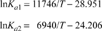
Stoichiometry
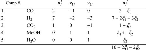
Imagine performing a flash at each new extent of conversion:
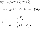
Writing objective functions:

This worksheet is called SMPRXN. An example of the output from a feed of 2,7,1,0,0 mole each of CO, H2, CO2, CH3OH, H2O is shown in Fig. 17.7.

Figure 17.7. Worksheet SMPRXN from workbook Rxns.xlsx for Example 17.15 at several temperatures.
The method of solving this problem is extremely similar to the DUALRXN problem. The only significant addition is an extra constraint equation which specifies that the vapor mole fractions must sum to unity. Note that ξ1 is greater than unity. This is because we have 2 moles of CO in the feed, so 1.3 moles converted is about 65%.
a. Note: The symbols a and b are simply regression coefficients, not the equation of state parameters a and b.
Example 17.16. NO2 absorptiona
The strength of concentrated acid which can be produced is limited by the back pressure of NO2 over the acid leaving the absorbers. The overall reaction, obtained by adding reactions (a) and (b), is shown as (c). Here we assume that N2O4 is equivalent to 2NO2.

The gas entering the bottom plate of a nitric acid absorber contains 0.1 mole of NO per mole of mixture and 0.25 mole of NO2 per mole mixture. The entering gas also contains 0.3 bar partial pressure of oxygen, in addition to inert gas. The total pressure is 1 bar. The acid made by the absorption operation contains 50% by weight of HNO3, and the operation is isothermal at 86°F. Estimate the composition of the gas entering the second plate and the strength of the gas leaving the second plate.
Solution
(Basis: 1 mole gaseous feed)
Assume yw = yHNO3 = 0 and xNO2 = xNO = 0.
For liquid:

For vapor:

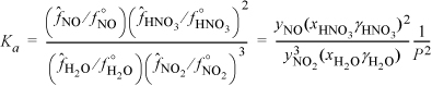
We can determine the mole fractions from the weight fractions:
Noting from the CRC Handbookb the vapor pressure of HNO3 is 64.6 mmHg, we can estimate the activity coefficients of HNO3 and water from the x-y data in The Chemical Engineers’ Handbook.c

Gibbs energies of formation are available in Appendix E for all but nitrogen dioxide, and Reid et al.d give the standard Gibbs energy of formation as 52 kJ/mol and the standard heat of formation as 33.87 kJ/mol. Performing a shortcut calculation using Kcalc.xlsx, the equilibrium constant at 303.15 K is Ka = 0.0054.
At P = 1 bar:
Substituting for the reaction coordinate:
Solving the cubic equation, ξ = 0.0431.
xHNO3 = (2ξ/(W + ξ) = 2·0.0431/(W + 0.0431) = 0.222 tells us that
W = –0.0431 + 2·0.0431/0.222 = 0.345 moles
So the composition of gas entering the second stage is yNO = 0.157; yNO2 = 0.132; yO2 = 0.328; yI = 0.383. Computations for further stages would be similar.
a. S. Lee, Personal Communication, 1993.
b. Weast, R.C. 1979. CRC Handbook of Chemistry and Physics, 60th ed, Boca Raton, FL: CRC Press, p. D-224.
c. Perry, R.H., Chilton, C.H. 1986. The Chemical Engineers’ Handbook, 6th ed. New York, NY: McGraw-Hill, p. 3–70.
d. Reid, R.C., Prausnitz, J.M., Poling, B. 1987. The Properties of Gases & Liquids, 4th ed, New York, NY: McGraw-Hill.
17.20. Summary
We have greatly enlarged the scope of our coverage of engineering thermodynamics with very little extension of the conceptual machinery. All we really did conceptually was recall that the Gibbs energy should be minimized. The provision that atoms can be moved from one chemical species to another with commensurate changes in energy and entropy simply means that reference states must be assigned to elemental standard states instead of standard states based on pure components, such that the free energies of all the components can be compared. In this sense we begin to comprehend in a new light the broad range of applications mentioned in Einstein’s quote at the end of Chapter 1. Instead of conceptual challenges, reaction equilibria focus primarily on the computational aspects of setting up and solving the problems. Notably, equation solvers can provide multidimensional capability. These are tools that can be adapted to many problems, even those beyond the scope of thermodynamics. You should familiarize yourself with such tools and build the expertise that will permit you to enhance your productivity.
Important Equations
The shortcut van’t Hoff equation provides a rapid method for screening the effect of temperature on the equilibrium constant. For best results, the temperature range should be limited as suggested in Section 17.8.

When combined with the equilibrium constraint Eqn. 17.15, reaction conversions can be estimated for many common scenarios.

The most common scenario is for ideal gases, because most industrial reactions are conducted at high temperature (to accelerate rates) and low pressure (to minimize cost).

For liquid phase components, we showed that the activity should be written as ai = xiγi. For solid species, we showed that the activity is unity when the solid is pure. The relevant Gibbs energy of formation must be used when liquids or solids appear in the equilibrium constant expression.
For simultaneous reaction and phase equilibria, we showed that the reaction could be treated in any one of the phases. Since the phase equilibrium constraint asserts equality of fugacity between phases, conceiving of the reaction in any particular phase is inconsequential, providing that the activities and Gibbs energies of formation use the same standard state.
Test Yourself
1. Reproduce the values given for the Gibbs energy of formation at 900 K for the component in Example 17.3. What values are given by the shortcut van’t Hoff equation?
2. Explain why a plot of lnK versus 1/T exhibits slight curvature.
3. When T is raised, the equilibrium constant is found to increase. Is the reaction endothermic or exothermic?
4. Explain why formation of a pure solid product does not inhibit a gas-solid reaction from going forward.
5. A reaction occurs with all components present in liquid and gas phases. Compositions in both phases are measured and the activities are calculated. The equilibrium constant value calculated using vapor phase activities is different from the equilibrium constant calculated using liquid phase activities. Is something wrong?
6. Describe the behavior of the reaction rate as equilibrium is approached. Explain why most industrial reactors are not run near equilibrium. Explain why calculation of an equilibrium constant is a good idea whenever designing a reactor.
17.21. Practice Problems
P17.1. An equimolar mixture of H2 and CO is obtained by the reaction of steam with coal. The product mixture is known as “water-gas.” To enhance the H2 content, steam is mixed with water-gas and passed over a catalyst at 550°C and 1 bar so as to convert CO to CO2 by the reaction:
Any unreacted H2O is subsequently condensed and the CO2 is subsequently absorbed to give a final product that is mostly H2. This operation is called the water-gas shift reaction. Compute the equilibrium compositions at 550°C based on an equimolar feed of H2, CO, and H2O.
Data for 550°C:

P17.2. One method for the production of hydrogen cyanide is by the gas-phase nitrogenation of acetylene according to the reaction: N2 + C2H2 ![]() 2HCN. The feed to a reactor in which the above reaction takes place contains gaseous N2 and C2H2 in their stoichiometric proportions. The reaction temperature is controlled at 300°C. Estimate the product composition if the reactor pressure is: (a) 1 bar; (b) 200 bar. At 300°C,
2HCN. The feed to a reactor in which the above reaction takes place contains gaseous N2 and C2H2 in their stoichiometric proportions. The reaction temperature is controlled at 300°C. Estimate the product composition if the reactor pressure is: (a) 1 bar; (b) 200 bar. At 300°C, ![]() .
.
P17.3. Butadiene can be prepared by the gas-phase catalytic dehydrogenation of 1-butene: C4H8 ![]() C4H6 + H2. In order to suppress side reactions, the butene is diluted with steam before it passes into the reactor.
C4H6 + H2. In order to suppress side reactions, the butene is diluted with steam before it passes into the reactor.
a. Estimate the temperature at which the reactor must be operated in order to convert 30% of the 1-butene to 1,3-butadiene at a reactor pressure of 2 bar from a feed consisting of 12 mol of steam per mole of 1-butene.
b. If the initial mixture consists of 50 mol% steam and 50 mol% 1-butene, how will the required temperature be affected?
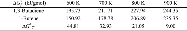
P17.4. Ethylene oxide is an important organic intermediate in the chemical industry. The standard Gibbs energy change at 298 K for the reaction ![]() mole. This large negative value of ΔGoT indicates that equilibrium is far to the right at 298 K. However, the direct oxidation of ethylene must be promoted by a catalyst selective to this reaction to prevent the complete combustion of ethylene to carbon dioxide and water. Even with such a catalyst, it is thought that the reaction will have to be carried out at a temperature of about 550 K in order to obtain a reasonable reaction rate. Since the reaction is exothermic, an increase in temperature will have an adverse effect on the equilibrium. Is the reaction feasible (from an equilibrium standpoint) at 550 K, assuming that a suitable catalyst selective for this reaction is available? For ethylene oxide, ΔHf298 = -52.63 kJ/mol. Heat capacity equations (in J/mole-K) for the temperature range involved may be approximated by CP,C2H4O = 6.57 + 0.1389 T(K); CP,C2H4 = 15.40 + 0.0937 T(K); CP,O2 = 26.65 + 0.0084 T(K)
mole. This large negative value of ΔGoT indicates that equilibrium is far to the right at 298 K. However, the direct oxidation of ethylene must be promoted by a catalyst selective to this reaction to prevent the complete combustion of ethylene to carbon dioxide and water. Even with such a catalyst, it is thought that the reaction will have to be carried out at a temperature of about 550 K in order to obtain a reasonable reaction rate. Since the reaction is exothermic, an increase in temperature will have an adverse effect on the equilibrium. Is the reaction feasible (from an equilibrium standpoint) at 550 K, assuming that a suitable catalyst selective for this reaction is available? For ethylene oxide, ΔHf298 = -52.63 kJ/mol. Heat capacity equations (in J/mole-K) for the temperature range involved may be approximated by CP,C2H4O = 6.57 + 0.1389 T(K); CP,C2H4 = 15.40 + 0.0937 T(K); CP,O2 = 26.65 + 0.0084 T(K)
P17.5. The water-gas shift reaction is to be carried out at a specified temperature and pressure employing a feed containing only carbon monoxide and steam. Show that the maximum equilibrium mole fraction of hydrogen in the product stream results when the feed contains CO and H2O in their stoichiometric proportions. Assume ideal gas behavior.
P17.6. Assuming ideal gas behavior, estimate the equilibrium composition at 400 K and 1 bar of a reactive gaseous mixture containing the three isomers of pentane. Standard formation data at 400 K are

P17.7. One method for the manufacture of synthesis gas depends on the vapor-phase catalytic reaction of methane with steam according to the equation ![]() . The only other reaction which ordinarily occurs to an appreciable extent is the water-gas shift reaction. Gibbs energies and enthalpies for the problem are tabulated below in kJ/mol.
. The only other reaction which ordinarily occurs to an appreciable extent is the water-gas shift reaction. Gibbs energies and enthalpies for the problem are tabulated below in kJ/mol.
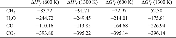
Compute the equilibrium compositions based on a 1:1 feed ratio at 600 K and 1300 K and 1 bar and 100 bars.
P17.8. Is there any danger that solid carbon will form at 550°C and 1 bar by the reaction 2CO = Cs + CO2? (ANS. Yes)
P17.9. Calculate the equilibrium percent conversion of ethylene oxide to ethylene glycol at 298 K and 1 bar if the initial molar ratio of ethylene oxide to water is 3.0.
C2H4O(g) + H2O(l) = (CH2OH)2 (1 M aq solution) ![]()
To simplify the calculations, assume that the gas phase is an ideal gas mixture, that γw = 1.0, and that the shortcut K value is applicable for ethylene oxide and ethylene glycol.
P17.10. Acetic acid vapor dimerizes according to 2A1 ![]() A2. Assume that no higher-order associations occur. Supposing that a value for Ka is available, and that the monomers and dimers behave as an ideal gas, derive an expression for yA1 in terms of P and Ka. Then develop an expression for PV/noRT in terms of yA1, where no is the superficial number of moles neglecting dimerization. Hint: Write no/nT in terms of yA1 where nT = n1 + n2.
A2. Assume that no higher-order associations occur. Supposing that a value for Ka is available, and that the monomers and dimers behave as an ideal gas, derive an expression for yA1 in terms of P and Ka. Then develop an expression for PV/noRT in terms of yA1, where no is the superficial number of moles neglecting dimerization. Hint: Write no/nT in terms of yA1 where nT = n1 + n2.
17.22. Homework Problems
17.1. For their homework assignment three students, Julie, John, and Jacob, were working on the formation of ammonia. The feed is a stoichiometric ratio of nitrogen and hydrogen at a particular T and P.
Julie, who thought in round numbers of product, wrote:
![]()
John, who thought in round numbers of nitrogen, wrote:
N2 + 3H2 ![]() 2NH3
2NH3
Jacob, who thought in round numbers of hydrogen, wrote:
![]()
a. How will John’s and Jacob’s standard state Gibbs energy of reactions compare to Julie’s?
b. How will John’s and Jacob’s equilibrium constants be related to Julie’s?
c. How will John’s and Jacob’s equilibrium compositions be related to Julie’s?
d. How will John’s and Jacob’s reaction coordinate values be related to Julie’s?
17.2. The simple statement of the Le Châtelier principle leads one to expect that if the concentration of a reactant were increased, the reaction would proceed so as to consume the added reactant. Nevertheless, consider the gas-phase reaction, N2 + 3H2 ![]() 2NH3 equilibrated with excess N2 such that N2′s equilibrium mole fraction is 0.55. Does adding more N2 to the equilibrated mixture result in more NH3? Why?
2NH3 equilibrated with excess N2 such that N2′s equilibrium mole fraction is 0.55. Does adding more N2 to the equilibrated mixture result in more NH3? Why?
17.3. The production of NO by the direct oxidation of nitrogen occurs naturally in internal combustion engines. This reaction is also used to produce nitric oxide commercially in electric arcs in the Berkeland-Eyde process. If air is used as the feed, compute the equilibrium conversion of oxygen at 1 bar total pressure over the temperature range of 1300–1500°C. Air contains 21 mol% oxygen and 79% N2.
17.4. The following reaction reaches equilibrium at the specified conditions.
C6H5CH = CH2(g) +H2(g) ![]() C6H5C2H5(g)
C6H5C2H5(g)
The system initially contains 3 mol H2 for each mole of styrene. Assume ideal gases. For styrene, ![]() ,
, ![]() .
.
a. What is Ka at 600°C?
b. What are the equilibrium mole fractions at 600°C and 1 bar?
c. What are the equilibrium mole fractions at 600°C and 2 bar?
17.5. For the cracking reaction,
C3H8(g) ![]() C2H4(g) + CH4(g)
C2H4(g) + CH4(g)
the equilibrium conversion is negligible at room temperature but becomes appreciable at temperatures above 500 K. For a pressure of 1 bar, neglecting any side reactions, determine:
a. The temperature where the conversion is 75%. [Hint: conversion = amount reacted/amount fed. Relate ξ to the conversion.]
b. The fractional conversion which would be obtained at 600 K if the feed to a reactor is 50 mol% propane and 50 mol% nitrogen (inert). (Consider the reaction to proceed to equilibrium.)
17.6. Ethanol can be manufactured by the vapor phase hydration of ethylene according to the reaction: C2H4 + H2O ![]() C2H5OH. The feed to a reactor in which the above reaction takes place is a gas mixture containing 25 mol% ethylene and 75 mol% steam.
C2H5OH. The feed to a reactor in which the above reaction takes place is a gas mixture containing 25 mol% ethylene and 75 mol% steam.
a. What is the value of the equilibrium constant, Ka, at 125°C and 1 bar?
a. Provide an expression to relate Ka to ξ. Solve for ξ.
17.7. Ethylene is a valuable feedstock for many chemical processes. In future years, when petroleum is not as readily available, ethylene may be produced by dehydration of ethanol. Ethanol may be readily obtained by fermentation of biomass.
a. What percentage of a pure ethanol feed stream will react at 150°C and 1 bar if equilibrium conversion is achieved?
b. If the feed stream is 50 mol% ethanol and 50 mol% N2, what is the maximum conversion of ethanol at 150°C and 1 bar?
17.8. The catalyzed methanol synthesis reaction, CO(g) + 2H2(g) ![]() CH3OH(g), is to be conducted by introducing equimolar feed at 200°C. What are the mole fractions and the temperature at the outlet if the system is adiabatic at 10 bar and the catalyst provides equilibrium conversion without any competing reactions?
CH3OH(g), is to be conducted by introducing equimolar feed at 200°C. What are the mole fractions and the temperature at the outlet if the system is adiabatic at 10 bar and the catalyst provides equilibrium conversion without any competing reactions?
17.9. A gas stream composed of 15 mol% SO2, 20 mol% O2, and 65 mol% N2 enters a catalytic reactor operating and forms SO3 at 480°C and 2 bar.
a. Determine the equilibrium conversion of SO2.
b. Determine the heat transfer required per mole of reactor feed entering at 295 K and 2 bar.
17.10. The feed gas to a methanol synthesis reactor is composed of 75 mol% H2, 12 mol% CO, 8 mol% CO2, and 5 mol% N2. The system comes to equilibrium at 550 K and 100 bar with respect to the following reactions:
2H2(g) + CO(g) ![]() CH3OHg)
CH3OHg)
H2(g) + Co2(g) ![]() CO(g) + H2O(g)
CO(g) + H2O(g)
Assuming ideal gases, derive the equations that would be solved simultaneously for ξ1, ξ2 where 1 refers to the first reaction listed. Provide numerical values for the equilibrium constants. Determine ξ1 and ξ2 ignoring any other reactions.
17.11. The 10/25/93 issue of Chemical and Engineering News suggests that the thermodynamic equilibrium in the isomerization of n-butene (CH3CH=CHCH3, a mix of cis and trans isomers) is reached at a temperature of 350°C using a zeolite catalyst. The products are isobutene and 1-butene (CH2=CHCH2CH3). The isobutene is the desired product, for further reaction to MTBE. Determine the equilibrium composition of this product stream at 1 bar.
17.12. Acrylic acid is produced from propylene by the following gas phase reaction:
![]()
A significant side reaction is the formation of acetic acid:
![]()
The reactions are carried out at 310°C and 4 bar pressure using a catalyst and air as an oxidant. Steam is added in the ratio 8:1 steam to propylene to stabilize the heat of reaction. If 50% excess air is used (sufficient air so that 50% more oxygen is present than is needed for all the propylene to react by the first reaction), calculate the equilibrium composition of the reactor effluent.
a. As part of a methanol synthesis process similar to problem 17.10, one side reaction that can have an especially unfavorable impact on the catalyst is coke formation. As a first approximation of whether coke (carbon) formation would be significant, estimate the equilibrium extent of coke formation based solely on the reaction: CO + H2 ![]() C(s) + H2O. Conditions for the reaction are 600 K and 100 bar.
C(s) + H2O. Conditions for the reaction are 600 K and 100 bar.
b. Is coke formation by the reaction from part (a) expected at the conditions cited in problem 17.10?
17.14. Hydrogen gas can be produced by the following reactions between propane and steam in the presence of a nickel catalyst:
C3H8 + 3H2O ![]() 3CO + 7H2
3CO + 7H2
CO + H2O ![]() CO2 + H2
CO2 + H2
Neglecting any other competing reactions:
a. Compute the equilibrium constants at 700 K and 750 K.
b. What is the equilibrium composition of the product gas if the inlet to the catalytic reactor is propane and steam in a 1:5 molar ratio at each of the temperatures and 1 bar?
17.15. Write and balance the chemical reaction of carbon monoxide forming solid carbon and carbon dioxide vapor. Determine the equilibrium constant at 700 K and 750 K. Will solid carbon form at the conditions of problem 17.14?
17.16. Catalytic converters on automobiles are designed to minimize the NO and CO emissions derived from the engine exhaust. They generally operate between 400°C and 600°C at 1 bar of pressure. K.C. Taylor (1993. Cat. Rev. Sci. Eng. 35:457.) gives the following compositions (in ppm, molar basis) for typical exhaust from the engine:
![]()
The additional products of the effluent stream include NO2, N2O, N2O4, and NH3. Estimate the compositions of all species at each temperature {400°C, 500°C, 600°C} and plot the ratio of NH3/CO as a function of temperature. (Note: Use the options of the Solver software to set the precision of the results as high as possible.)
17.17. Styrene can be hydrogenated to ethyl benzene at moderate conditions in both the liquid and the gas phases. Calculate the equilibrium compositions in the vapor and liquid phases of hydrogen, styrene, and ethyl benzene at each of the following conditions:
a. 3 bar pressure and 298 K, with a starting mole ratio of hydrogen to styrene of 2:1
b. 3 bar pressure and 423 K, with a starting mole ratio of hydrogen to styrene of 2:1
c. 3 bar pressure and 600 K, with a starting mole ratio of hydrogen to styrene of 2:1
17.18. Habenicht et al. (1995. Ind. Eng. Chem. Res., 34:3784) report on the reaction of t-butyl alcohol (TBA) and ethanol (EtOH) to form ethyltertiary-butyl ether (ETBE). The reaction is conducted at 170oC. A typical feed stream composition (in mole fraction) is:
![]()
Isobutene is the only significant by-product. Assuming that equilibrium is reached in the outlet stream, estimate the minimum pressure at which the reaction must be conducted in order to maintain everything in the liquid phase. Do isobutene or ETBE exceed their liquid solubility limits at the outlet conditions?
17.19. Limestone (CaCO3) decomposes upon heating to yield quicklime (CaO) and carbon dioxide. At what temperature does limestone exert a decomposition pressure of 1 bar?
17.20. Two-tenths of a gram of CaCO3(s) is placed in a 100 cm3 pressure vessel. The vessel is evacuated of all vapor at 298 K and sealed. The reaction CaCO3(s) = CaO(s) + CO2(g) occurs as the temperature is raised. At what temperature will the conversion of CaCO3 be 50%, and what will the pressure be?
17.21. One suggestion for sequestering CO2 is to synthesize carbonate polymers. Polycarbonate is well known for its strength and transparency. To gauge the feasibility of this approach, consider the synthesis of dimethyl carbonate (DMC) from methanol and CO2 at 350 K.
a. Write a balanced stoichiometric equation for this reaction. Highlight any by-products.
b. Estimate the Ka value for the reaction. What pressure is required to achieve P·Ka = 0.1?
c. Methanol and DMC are both liquids at this temperature. Explain how to estimate their partial pressures at a given extent of conversion. You may neglect the CO2 in the liquid for this question.
17.22. Ethyl acetate is to be produced by a liquid phase reaction.
a. Use the shortcut van’t Hoff equation to calculate the expected conversion of HOAc for equimolar feeds of EtOH and HOAc in a batch reactor at 80°C.
b. Repeat part (a) with a 3:1 ratio of EtOH to HOAc at 80°C.
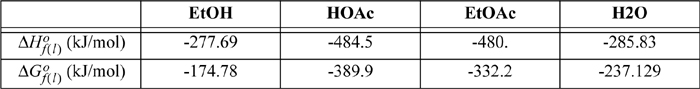
17.23. Hamilton, et al.,6 have studied the binding of DNA chromosomes to proteins WT1 and EGR1. WT1 uses a zinc binding site to suppress a certain type of kidney tumor. EGR1 binds to regulate cell proliferation. There may be an important regulatory link between the two proteins.7

a. Use the binding data above to determine the standard state Gibbs energies of reaction at each temperature, the heat of reaction over the temperature range, and the entropy of reaction over the temperature range.
b. The binding constants are about the same size. Evaluate the relative magnitudes of the enthalpy and entropy of formation for each binding type. Does the thermodynamic analysis imply that the binding types are similar or different?
17.24. The enthalpy of reaction for many biological reactions and surfactants is strongly temperature-dependent, but instead of using full heat capacities, the temperature dependence can be characterized by differences in heat capacities ΔCP = CP,prod – CP,react, typically assumed to be independent of temperature.7
a. The heat of reaction is represented by ΔH = ΔHR + ΔCP(T – TR). Show that
b. Provide an equation consistent with part (a) for the temperature dependence of the entropy of reaction.
17.25. Lysozyme (MW = 14.313 kDa) undergoes a phase transition from a native folded (N) to unfolded state (U) that can be considered a reversible reaction, N(aq) ![]() U(aq), where the subscript (aq) indicates that the protein is in an aqueous solution. At high temperature the protein is in state U and at low temperature, it is in state N. The melting temperature (Tm) is where the concentrations are equal. The melting temperature can be changed by pH, ionic strength (added salt), denaturant (solvents), or pressure. The results of problem 17.24 apply. The protein unfolding has been studied by Cooper, et al.8 The heat to unfold 1 mg/mL of protein in 2 mL of pH = 4 solution at Tm = 78°C is 0.0755 J, ΔCP = 6.3 kJ/mol-K. The ΔV = –40 mL/mol.7
U(aq), where the subscript (aq) indicates that the protein is in an aqueous solution. At high temperature the protein is in state U and at low temperature, it is in state N. The melting temperature (Tm) is where the concentrations are equal. The melting temperature can be changed by pH, ionic strength (added salt), denaturant (solvents), or pressure. The results of problem 17.24 apply. The protein unfolding has been studied by Cooper, et al.8 The heat to unfold 1 mg/mL of protein in 2 mL of pH = 4 solution at Tm = 78°C is 0.0755 J, ΔCP = 6.3 kJ/mol-K. The ΔV = –40 mL/mol.7
a. What is the Gibbs energy change for the unfolding at the melting temperature? (Hint: The answer requires conceptual thought, not many calculations.)
b. Show that at the melting temperature at pH = 4, ΔH = 540 kJ/mol and ΔS = 1.54 kJ/mol.
c. Evaluate the contributions to ΔG at 23°C and pH = 4. Is the process driven by enthalpy or entropy under these conditions?
d. Show that the relation for [N]/[U] is ![]() For a solution of overall concentration 1 mg/mL, plot [U] as a function of temperature for 20 ≤ T ≤ 110 °C, and provide a tabular summary of [U] at 60°C and 90°C.
For a solution of overall concentration 1 mg/mL, plot [U] as a function of temperature for 20 ≤ T ≤ 110 °C, and provide a tabular summary of [U] at 60°C and 90°C.
e. When pH is varied, the net charges on the protein change (as will be explained in Chapter 18), resulting in different Tm and ΔH. In the range 20 ≤ Tm ≤ 78 °C, the relation is ΔH(kJ/mol) = 48.6 + 6.3 Tm(°C). Derive the relation between ΔS and Tm.
f. At pH = 1, Tm = 43°C. Provide a plot of plot [U] as a function of temperature for 20 ≤ T ≤ 110 °C, and provide a tabular summary of [U] at 25°C and 55°C.
g. (advanced) Lysozyme has four disulfide bonds that are important in the folding behavior. The authors created a mutant protein with only three disulfide bonds. The relation in (e) still holds. At pH = 2.5, Tm = 23°C for the mutant. Evaluate the contributions of enthalpy and entropy to the folding.
h. (advanced) Provide an interpretation for the sign of ΔV. At pH = 4, how much pressure is needed to lower the melting temperature 5°C to 73°C?9
17.26. Surfactants clump together to form organized structures called micelles that can be spheres, rods, and so forth. The formation of the clump can be modeled as a “chemical” reaction, though there are no chemical bonds formed or broken. When surfactants are in solution below the critical micelle concentration, CMC, the surfactant molecules are almost all “free” in solution. At the CMC, micelles start to form. Above the CMC, the amount of free surfactant is almost constant in solution and as more surfactant is added to the solution, more micelles form. It is conventional to provide the property changes of surfactants per mol of surfactant molecules, not per mole of micelle.
a. Given the data below for nonylglucoside (NG) demicellization in water, calculate the micellization value, ΔCPmic, as a function of temperature. Is the heat capacity of a micelle greater than or less than the heat capacity of the molecules that make up the micelle?
b. Calculate ΔSmic and for the surfactant as a function of temperature. Is the overall solution (including water) more ordered or less ordered after micellization?
NG data:

17.27. Micelle formation in surfactants is described in problem 17.26. Solve the problem using the data for sodium docecyl sulfate, SDS in water.
SDS data:

17.28. For nonylglucoside, NG, thermodynamic data for demicellization in water are presented in problem 17.26. Model the micelle reaction as nS ![]() Mn where S is free surfactant and Mn is a micelle. Treat the solution as an ideal solution. Vary the total concentration of NG from 0 up to 20 mmol/L. Water is 55.5 mol/L. Calculate mole fractions and molar concentrations (mmol/L) of the free surfactant (in mM) and the micelles (in μM) of NG at T=285 K, where n = 58. Plot curves for the concentrations. Identify the approximate CMC in mmol/L. Hint to simplify calculations: The mol/L added is very small relative water molarity (55.5 mol/L). The density can be assumed to be constant.
Mn where S is free surfactant and Mn is a micelle. Treat the solution as an ideal solution. Vary the total concentration of NG from 0 up to 20 mmol/L. Water is 55.5 mol/L. Calculate mole fractions and molar concentrations (mmol/L) of the free surfactant (in mM) and the micelles (in μM) of NG at T=285 K, where n = 58. Plot curves for the concentrations. Identify the approximate CMC in mmol/L. Hint to simplify calculations: The mol/L added is very small relative water molarity (55.5 mol/L). The density can be assumed to be constant.