
7. Capital Budgeting and Discounted Cash Flow Analysis
Discounted cash flow analysis is probably the most important financial tool that you will encounter. Fortunately, present values are easy to understand and easy to calculate. If you had the opportunity to choose between receiving $1,000 a year from today or receiving $1,000 today, which would you prefer? Clearly you would prefer to receive the cash today. If you received the money today, you could invest it and earn a return during the upcoming year. If you could invest at 5%, at the end of the year you would have $1,050 (your original $1,000 plus $50 in interest). So if 5% is the correct interest rate, a choice between $1,000 a year from now and $1,000 today is equivalent to a choice between $1,000 a year from now and $1,050 a year from now. Obviously, $1,050 is the better outcome. A dollar received today is always worth more than a dollar received in the future. The sooner you receive the money, the sooner you can invest it and begin receiving a return or borrow less and avoid paying out interest.
Calculating Present Values
You’ll no doubt hear financial analysts referring to the present value of future cash flows. The present value of any future amount is just the amount you would have to invest today to grow to that future amount in the assumed time period at the assumed interest rate. So at 5% interest, $1,000 is the present value of $1,150 to be received 2 years from now. This relationship can be summarized by the equation in Exhibit 7-1. In this equation, the interest rate is expressed in decimal form (5% = .05), and t is the number of years the funds remain invested.
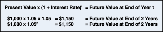
Exhibit 7-1. Relationship between present value and future value
This equation is nothing more than a sixth-grade compound interest formula. Fortunately, that’s all you need to calculate present values and perform discounted cash flow analyses. You will usually find it more convenient to work with that equation if you rearrange the terms. When you divide both sides of that equation by (1 + Interest rate)t you get
Present value = Future Value / (1 + Interest rate)t
Using that expression, it is straightforward to calculate the present value of any future amount.
Discounted Cash Flow Analysis (DCF)
Present values are sometimes referred to as discounted cash flows (DCFs), and the interest rate is sometimes referred to as the discount rate. Financial models that utilize present value calculations are therefore often referred to DCF analyses. Capital budgeting is the process corporations use to determine whether long-term investments are worth pursuing. This typically involves calculating the DCF valuation of each potential project. Discounted cash flow analyses are essential tools for assessing almost all corporate expenditures. Examples could range from deciding which copy machine to purchase, to assessing the costs and benefits of an employee training program, to evaluating merger and acquisition (M&A) opportunities. It is, of course just as important to consider the time value of money when making personal financial decisions such as buying a house, saving for a child’s education, or choosing whether to buy or lease a new car. DCF techniques are also used to value financial instruments such as stocks, bonds, and employee stock options. The basic concepts are illustrated next, and specific applications are discussed in later chapters.
Reading a Present Value Table
Present value tables are tools that were created to reduce the amount of arithmetic involved in DCF calculations. They are seldom still used for that purpose because financial calculators and spreadsheets are now much better alternatives. However, before moving on to spreadsheets, the present value table in Exhibit 7-2 illustrates some basic time value of money concepts. Interpreting the numbers in the present value table is straightforward. If you think of the column headings as annual interest rates, you can think of the row headings as years. If the column headings were monthly interest rates, the row headings would represent months. Determining what interest rate to use is extremely important and is a topic discussed in detail later in this chapter in the section, “Selecting the Appropriate Discount Rate.” For the moment, assume the relevant annual interest rate is 10%. The table tells you that the present value of $1.00 received 1 year from now is .909 dollars, or just under 91 cents. That figure was calculated by dividing $1.00 by 1.10. If you put $.91 into an account earning 10%, at the end of 1 year your account balance would be $1.00. The table shows that the present value of $1 received 2 years from now is .826 dollars, or just under 83 cents ($1.00 / 1.102). The present value of $1 received 3 years from now is .751 dollars, or just more than 75 cents ($1.00 / 1.103). All other entries in the table were calculated in the same way.
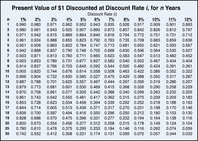
Exhibit 7-2. Present value table
Basic Time Value of Money Concepts
So how can you use this present value table? If the table tells you the present value of $1 received in the future, you can calculate the present value of any number of dollars. Suppose you want to buy your daughter a $1,000 computer when she graduates from high school 1 year from now. How much would you need to put in a bank account tomorrow morning at 10% to have that $1,000 ready when she graduates? You would need to deposit $909 ($1000 × .909), which is the present value of $1,000 received or paid 1 year from now. How much would you need to invest today if she were not going to graduate for 10 years? The present value of $1,000 in 10 years is only $386 ($1000 × .386). You would need to invest much less today because 10 years of compound interest, instead of just 1, would be added before you make your withdrawal. Other things equal, the present value will always be less when the time period is longer. Other things equal, the present value will always be larger when the interest rate is smaller. Suppose you will need $1,000 in 10 years but the annual return on your investment will be only 2%. You would need to invest $820 ($1000 × .820) instead of $386. That makes sense. If your investment will be growing more slowly, you need to start with an amount closer to your eventual target. When you start modeling corporate operating and strategic investments, it will be important to remember that, other things equal, a longer time period always reduces the present value of a future amount, and a lower interest rate always increases the present value of a future amount.
Do the Future Benefits Justify the Upfront Costs?
Now assume that your time value of money is 10%, for example, your money is currently in an account earning 10% per year. The most you should pay for a $1,000 benefit to be received 1 year from now is $909. If you had to pay more than that, you would be better off leaving the money in the account where it was earning 10%. In that account any amount greater than $909 would grow to more than $1,000 by the end of the year. Similarly, if your firm’s weighted average cost of capital were 10%, $909,000 is the most it should pay for a benefit of $1,000,000 to be received 1 year from now. If that same $1,000,000 benefit would not be received for 10 years, the most your firm should pay is $386,000.
Calculating the Present Value of a Series of Cash Flows
The same approach you have used to calculate the present value of a single payment can be used to calculate the present value series of cash flows. Suppose you have just learned that you won $1,000,000 in the New Jersey State lottery. You rush to the lottery commission office to pick up your $1 million check. They say, “Sorry, that’s not how it is done.” They explain that they will pay you $50,000 per year for the next 20 years and that $50,000 × 20 is $1,000,000. What lump sum amount would you be willing to accept today instead of receiving $50,000 per year for the next 20 years? This calculation is shown in Exhibit 7-3. The first two columns show the year and the amount to be received at the end of each year. The third column shows the 10% present value discount factors obtained from Exhibit 7-2. The right column is the product of the cash flow in each year and the present value discount factor for that year. For example, $45,455 is how much you would have to invest today to grow to $50,000 at the end of 1 year. If your time value of money is 10%, you would be indifferent between receiving $45,455 today or $50,000 1 year from now. This table also illustrates how dramatic the impact of compound growth rates can be. You would be indifferent between receiving the final $50,000 payment or only $7,432 today. That’s true because if you put $7,432 in an account earning 10%, it would after 20 years grow to exactly $50,000. The present value of the series of twenty $50,000 payments, the sum of the numbers in the right column, is $425,678. If your time value of money is 10%, you would be indifferent between receiving $425,678 today or $1 million spread out in $50,000 payments over the next 20 years. For the moment you are ignoring taxes and risk. Those factors are discussed in later chapters.
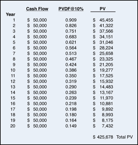
Exhibit 7-3. Calculating the present value of a series of payments
Using DCF on the Job
In case you don’t get to use this analysis in exactly that context, look at some work-related examples. Your colleague has calculated that if your firm were to purchase a more energy-efficient heating and cooling (HVAC) system for its corporate headquarters, it could reduce its energy bills by $50,000 per year for the next 20 years. He has also determined that a system with the appropriate energy efficiency rating and the necessary heating and cooling capacity would cost $600,000. He’s proud of the memo he has written to the boss recommending that the firm spend the $600,000 to achieve $1,000,000 in energy savings. If your firm’s weighted average cost of capital is 10%, would the investment he is recommending be a cost-effective one? No, if energy cost reductions are the only reason for putting in the new system, the most your firm should spend for the new system is $425,678. A basic premise of DCF analysis is that the economic value of any asset is the present value of the cash flows you receive as a result of owning that asset. That’s true whether the asset is an HVAC system, a piece of investment real estate, a share of stock, a bond, or even a company that you plan to acquire.
HR Applications
Here are some HR illustrations using the same numbers. Today is your 65th birthday, and you are about to retire. Under the terms of your company’s defined-benefit pension plan, you have a choice of receiving a $50,000 per year pension payment for the rest of your life or a one-time upfront lump sum payment of $450,000. If you assume that you will live for 20 years after you retire and that your time value of money is 10%, which alternative would you choose? Under those assumptions you would be better off taking the $450,000 upfront. Exhibit 7-3 showed that if you put $425,678 into an account earning 10% and then withdrew $50,000 at the end of each year, you would exactly empty that account at the end of the 20th year. That’s true because the $425,678 is the sum of the $45,455 that you would have to put in to grow to the first $50,000 withdrawal, the $41,322 needed to cover the second $50,000, and the amount needed to cover each of the other 18 withdrawals. If $425,678 is how much you have to deposit inured to draw out $50,000 per year, with a $450,000 deposit you could withdraw more than $50,000 in each of the next 20 years. That example could just as easily have been worded, “What’s the most you should spend on a training program that will increase workforce productivity by $50,000 per year in each of the next 20 years?” or “What’s the most you should spend on a HRIS program that will in each of the next 20 years eliminate the need for one data-entry position costing $50,000?” Of course, you may argue quite reasonably that you’ve never seen a software package with a useful life of 20 years. If the software package has a 3-year useful life, you just add up the first three rows ($45,455 + $41,322 + $37,556 = $124,343). These are generic models that can be easily customized to fit almost any business investment you are considering. If appropriate, a different cash flow could be entered for each year, and the number of years could be adjusted to reflect the length of the benefit stream you expect.
How Important Is It to Consider the Time Value of Money?
You need to consider the time value of money whenever you are comparing, adding, subtracting, or performing any calculations on cash flows that occur during different time periods. A mile is not equal to a kilometer, so you would not add one distance expressed in miles to another distance expressed in kilometers. The result would be meaningless. Before doing any calculations on those two numbers, you would need to express them both in the same unit of measurement, that is, both in miles or both in kilometers. Just as a mile is always bigger than a kilometer, a dollar received today is always worth more than a dollar received in the future. So before performing any calculations involving cash flows from different time periods, you need to express them in the common metric of present value.
Individuals sometimes assume that time value of money adjustments are only of real-world importance when the time horizons are long. For example, constructing a new manufacturing facility or starting an R&D project that might produce cash flows over a 20- or 30-year time frame. Now look at the example described in Exhibit 7-4 that involves a much shorter time horizon. In a past labor negotiation, the Chrysler Corporation offered the 70,000 members of its UAW collective-bargaining unit immediate lump sum bonuses averaging $2,120 each. How much more would it have cost Chrysler to increase its lump sum offer to $2,250, but spread the payments out over the 3-year life of the labor contract? Assume that at the time Chrysler’s WACC was 10% and that under the second option the $750 payments would be made at the end of each contract year. Because Option A involves only an immediate payment, there is no present value adjustment required. To calculate the present value of the series of payments under Option B, multiply each payment by the appropriate discount factor from the 10% column of the present value table in Exhibit 7-2. You see that Chrysler, given its 10% cost of raising money, would be indifferent between paying each worker $1,865 up front, or $750 at the end of each of the next 3 years. Now that both options have been expressed in present value terms, you can compare them. Option B costs $256 less per worker. Because at the time Chrysler had 70,000 active employees, increasing its offer to $2,250 would have saved Chrysler almost $17.8 million! If you had ignored the time value of money, you would have mistakenly concluded that $2,250 over the term of the contract was more expensive than $2,120 upfront. This example demonstrates that even over relatively short time horizons ignoring the time value of money can lead to seriously flawed decisions.
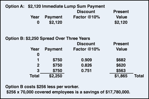
Exhibit 7-4. Using present value to compare alternative compensation schemes
Still need to convince yourself how real that $17.8 million savings is? Suppose Chrysler were to immediately deposit into a bank account earning 10% the amount needed to fund Option A and the amount needed to fund Option B. To fund Option A would require depositing 70,000 × $2,120. To fund Option B would require depositing 70,000 × $1,865. Do the math. That’s a $17.8 million difference. Less is needed to fund Option B because the initial deposit would grow by 10% before the first $750 payments are made. The remainder would grow by another 10% in year 2 before the second payment is made, and the balance would grow by 10% in the third year before the last payment is made. The effect would be exactly the same as in that hypothetical, but a more likely scenario would be that instead of pre-funding these payments and investing the funds at 10%, the firm would simply not need to raise the money immediately, avoiding the 10% cost of capital on those amounts.
Using Spreadsheets to Calculate Present Values
Although present value tables may be useful for illustrating how DCF models work, they are no longer the most efficient way to calculate them. The analysis in Exhibit 7-3 could be accomplished easily using the time value of money functions built into Microsoft Excel and most other spreadsheet programs. Exhibit 7-5 shows an Excel spreadsheet that does this. The cash flows are typed into any range of cells you prefer, and then in any cell you type the Excel formula to calculate the net present value of those cash flows. The general syntax of the Excel net present value formula is
=NPV(Interest rate, Range of cells
where the cash flows are located)
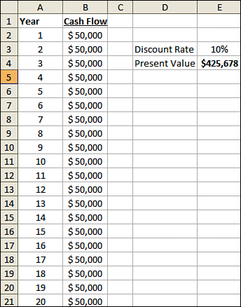
Exhibit 7-5. Using an Excel spreadsheet to replicate analysis in Exhibit 7-3
In Exhibit 7-5 the formula in cell E4 is =NPV(.10,B2:B21). The result returned is the same $425,678 that you calculated in Exhibit 7-3. An alternative formula that would produce exactly the same result is =NPV(E3,B2:B21). In this second formula the interest rate is replaced with a cell address showing where the interest rate is located. The advantage of this second approach is that you can more easily plug in different discount rates to determine their impact on the present value. For example in this case, lowering the interest rate from 10% to 5% increases the present value to $623,111. If this firm could raise money only at 10%, it should pay no more than $425,678 for this stream of benefits. If this firm could raise money at a cost of 5%, it could pay up anything to $623,111 for the same stream of benefits. Obviously, a business deal is more attractive if the funds used to finance it can be raised at a lower cost.
In the earlier lottery example, you assumed the $50,000 payment was received at the end of each year. If those amounts were received at the start of each year, you could adjust the spreadsheet, as shown in Exhibit 7-6. Note the difference is that only 19 cash flows are listed in Column A. Because the first $50,000 would be received at the beginning of the first year, there is no time value of money adjustment required for that amount. The second payment would be received at the end of year 1 (the start of year 2), the third payment at the end of year 2, and so forth. The 20th payment would be received at the end of the 19th year. The present value of the 20 payments ($468,246) is therefore the initial $50,000 plus the $418,246 present value of the 19 future cash flows.
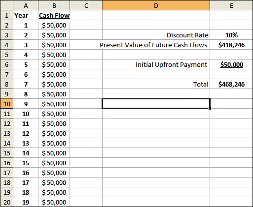
Exhibit 7-6. Present value when cash flows occur at beginning of each period
Example of Using Excel’s NPV Function to Analyze a Buy Versus Lease Decision
Now look at a buy versus lease analysis using Excel’s built-in NPV function. You have decided that you need a new BMW 328i. The dealer says he agrees with you and explains that he has two ways that he can help you get that car. He will be glad to sell you the car for $35,200, or he will be equally happy to lease it to you. The 4-year lease would require an immediate $5,000 down payment, and then payments of $5,400 at the end of each year. Assume all funds will be taken out of an account earning 8% per year. The first step is to write down the pattern of cash flows associated with each alternative, as shown in Exhibit 7-7. The negative numbers represent cash you will have to pay out, and the one positive number, $18,300, is what you estimate you will receive if you sell the car at the end of year 4. The formula typed into cell B9 is =B2+NPV(0.08, B3:B6). The formula typed into cell C9 is =C2+NPV(0.08, C3:C6). In both cases the initial payment occurs at the present and is therefore not included in the range of cells specified in the NPV function. Excel assumes that the first entry in an NPV range is one period out, that the second is two periods out, and so forth. Had the $35,200 purchase price or the $5000 down payment been included within the NPV range, Excel would have treated them as occurring one year from now. The results in Exhibit 7-7 indicate that with this particular set of assumptions, buying the car would be approximately $1,000 cheaper than leasing it. Suppose however that you were taking the funds out of an account earning 15% or that you were borrowing the money from your brother-in-law who was charging you 15%. To make this change you would simply alter the NPV formulas to =B2+NPV(0.15, B3:B6) and =C2+NPV(0.15, C3:C6). At this higher cost of capital, the buy option becomes the more expensive one. Does that make intuitive sense? The buy option requires you to commit a much larger amount up front. The greater your cost of capital is, the greater the cost of tying that much cash up right away.
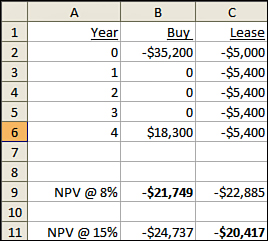
Exhibit 7-7. Lease or buy a BMW 328i
Determining the Relevant Cash Flows
An important aspect of the previous example is that it assumed the same end points under both alternatives, that is, that you did not own the car at the end of the 4 years. You sold it after 4 years under the buy option or turned it in after 4 years under the lease option. Had you not modeled equivalent end points, you would not be evaluating just the difference between buying and leasing. You would have also included the difference between owning and not owning the car at the end of year 4. If the objective is to isolate the cost differences between buying and leasing, you must model the same end point under both alternatives.
Another key assumption in the previous example was the choice of the 4-year time horizon. How could you model the cash flows if you were not sure whether you would keep this new car for 4, 6, or even 10 years? The approach shown in Exhibit 7-8 accommodates that scenario by assuming that you will own the car after 4 years under both options. Under the buy option you do not sell it and therefore receive no cash at the end of year 4. Under the lease option you purchase the car at the end of the lease for (you can assume) $19,000 and therefore pay out $24,400 ($19,000 plus the final lease payment of $5,400). Because under both alternatives you own the car at the end of year 4, how long you keep it after that is irrelevant to the original buy versus lease choice.
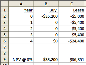
Exhibit 7-8. Lease/buy analysis when the time frame is unclear
Should maintenance costs be included in the model when analyzing the buy-versus-lease decision? Yes, if maintenance costs would be different under the buy and lease options. No, if maintenance costs would be the same under both the buy and lease options. When constructing DCF analyses you can determine whether a particular cash flow needs to be considered using what is sometimes referred to as the with-without rule. The only relevant cash flows are those that differ with a particular choice versus without that choice. For example, suppose you must pay for gasoline whether you buy the car or lease a car. The cost of the gas is real. It’s just not relevant to the choice between buying or leasing the car.
Selecting the Appropriate Discount Rate
The interest rate in present value calculations is often referred to as the discount rate. The appropriate discount rate is the one that reflects the decision-maker’s opportunity cost of capital, in other words how much the decision-maker could have benefited from the use of this money had it not been committed to this project. If the cash is already on hand, the appropriate discount rate is the rate of return you could have earned on alternative investments. If cash must be raised to undertake this project, the appropriate discount rate is the rate that must be paid to obtain those funds. The logic is the same whether the decision-maker is a for-profit corporation, a nonprofit organization, or you or your family. If you’re going to make the payments on a car lease by taking the funds out of your bank account, the appropriate discount rate is the amount you would have earned had the money remained in that account. If you are going to make those payments by borrowing the money from your brother-in-law, the appropriate discount rate is the interest rate he charges you on that loan.
As discussed in Chapter 6, “Stocks, Bonds, and the Weighted Average Cost of Capital,” most corporations are financed through a combination of debt and equity. The weighted average of the cost of debt and the cost of equity is the firm’s cost of capital (WACC). The WACC is the interest rate that firms typically use when conducting discounted cash flow analyses. An important exception would be situations in which the investment being considered is of greater risk than the activities usually undertaken by that corporation. In such cases a risk-adjusted interest rate, one higher than the company’s WACC, would be more appropriate. Incorporating risk considerations into DCF analyses is discussed in Chapter 9, “Financial Analysis of a Corporation’s Strategic Initiatives.”
Money Has Time Value Because of Interest Rates, Not Because of Inflation
A dollar received in the future is always worth less than a dollar received today. That would be true even if you lived in a zero inflation world. Money has time value because if you receive it sooner, you can either invest it and earn interest or borrow less and avoid paying interest. If you lived in a zero inflation world, interest rates would be lower, but they would still exist. You would still need to make time value of money adjustments. Nominal interest rates, those that exist in the marketplace, are themselves affected by inflationary expectations. For example, a banker who requires a 2% real return and expects inflation to average 7% might offer you a mortgage at 9%. If the banker had expected inflation to average only 4%, she could have offered you a 6% mortgage. When performing DCF analyses you can use either real, that is, inflation-adjusted, interest rates or nominal interest rates, but you need to be consistent. If you project cash flows that do not include anticipated future price changes, you need to discount those using real interest rates. If you project nominal cash flows, you need to discount those using nominal interest rates. This second approach is usually the easier one for managers to understand and work with. Project the dollar amounts you think you will actually receive or have to pay in future years, and discount those using the firm’s nominal weighted average cost of capital.
Using NPV to Evaluate an Investment or Project
Consider the example shown in Exhibit 7-9. This project involves a $100,000 upfront cost and then produces the benefits shown in years 1 through 5. The formula in cell B9 is =+B2+NPV(A11,B3:B7). Remember that because the –$100,000 shown in cell B2 is an immediate expenditure, it is not included within the range of cells specified within the NPV function. Excel assumes the first entry in that range is 1 year into the future. If this firm’s weighted average cost of capital is 12%, this project would have an NPV of $17,513. In other words, the net benefit to shareholders from this project is $17,513. The present value of the benefits in years 1 to 5 is $117,513, which is $17,513 more than the $100,000 initial cost. An investment is attractive when its NPV is greater than zero because that indicates that the present value of future benefits is greater than the upfront costs.
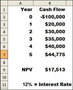
Exhibit 7-9. Find the interest rate that makes the NPV = 0
IRR as an Alternative to Net Present Value
To make investment decisions using NPV analyses, you must start with an assumption about the appropriate discount rate. The internal rate of return (IRR) approach reverses that sequence. Instead of starting with an estimate of the appropriate discount rate, this approach calculates the largest rate that could be used and still have the investment be an attractive one. At any cost of capital less than the IRR the project is worth pursuing; that is, the present value of the future benefits is greater than the upfront cost. At any cost of capital greater than that, the project is not worth pursuing; that is, the present value of the future benefit is less than the costs. Suppose you returned to the spreadsheet in Exhibit 7-9 and change the value in cell A11 to 14%. Discounting the benefits at this higher rate, the NPV would fall to $11,190. If you continued to incrementally increase the interest rate in cell A11, you would see that as you discount the future benefits at higher and higher rates, the NPV continues to decline. As shown in Exhibit 7-10, at an interest rate of 18%, the NPV reaches zero, and at any interest rate larger than 18%, the NPV is negative. The interest rate that makes the NPV equal the zero is defined as the IRR (see Exhibit 7-11).
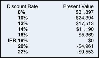
Exhibit 7-10. Present value of cash flows shown in Exhibit 7-9, calculated at different discount rates
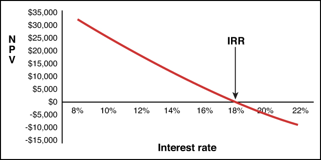
Exhibit 7-11. IRR is the interest rate that makes NPV = 0.
Using Excel’s Built-In IRR Functions
Exhibit 7-10 used a trial-and-error process to find the IRR. You can always begin by plugging a discount rate into the NPV formula and observing whether the resulting NPV is a positive number. If it is, you could keep trying larger and larger discount rates until the NPV dropped to zero. If the initial NPV estimate were a negative number, you could plug in successively smaller discount rates until the NPV rose to zero. A more efficient approach would be to use Excel’s built-in IRR function. The spreadsheet in Exhibit 7-12 contains the same cash flows shown in Exhibit 7-9. The general syntax of the Excel formula for calculating an internal rate of return is
=IRR(range of cells where the cash flows are located)
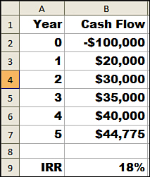
Exhibit 7-12. Using Excel’s built-in IRR function
The formula in cell B9 of the spreadsheet in Exhibit 7-12 is = IRR(B2:B7). Note that when working with the IRR function, the time zero cash flow is included in the range. The result calculated in cell B9 is exactly the same 18% you found by trial and error in Exhibit 7-10.
IRR analyses are popular with CFOs and line executives for at least two reasons. In many cases, they enable you to avoid having to make estimates of the appropriate discount rate. For example, there might be a disagreement within the finance department about whether the NPV of a particular project should be calculated using a discount rate of 10%, 12%, or 14%. If you know the project has an IRR of 18%, you won’t need to worry about resolving that disagreement. The project would add economic value to the firm at any of those rates and at any discount rate up to 18%. A second way IRR analyses are often used is to rank alternative investments. Giving up a project with an IRR of 20% would make economic sense if that were necessary to undertake a project with an IRR of 30%.
Two Different Ways to Answer the Same Question
To summarize you have considered two alternative decision rules. To utilize the NPV decision rule, you must begin with an estimate of cash flows and an estimate of the appropriate discount rate. Using the IRR decision rule, on the other hand, does not require you to begin with an estimate of the appropriate discount rate. Instead, this approach calculates the largest discount rate that could be applied to these cash flows and still have their present value be large enough to offset the project’s upfront costs. These two rules can be summarized as follows:
NPV decision criteria: Invest if NPV > zero
IRR decision criteria: Invest if IRR > WACC
The following example illustrates the use of these techniques to analyze financial securities such as bonds. Subsequent chapters utilize these two decision rules to evaluate HR initiatives and corporate operating and strategic investments.
Example of Using NPV to Price the Bonds in Your 401(k)
Suppose today is June 30, 2013, and your broker phones to suggest a bond she believes you should purchase for your 401(k). The bond that was originally issued in 2003 has a $1,000 par value, a coupon rate of 6%, and a maturity date of July 1, 2018. If you purchase the bond, the par value is the amount you will receive when the bond matures. The coupon rate is the percentage of par value the bond issuer promises to pay you annually as interest. The coupon rate was established based on market conditions existing at the time the bond was issued and is locked in for the life of the bond. The individual who purchased this bond in 2003 is now eager to sell it to you. How much would you pay for a $1,000 par value bond with a 6% coupon that will mature in another 5 years? That, of course, depends on what bonds of comparable riskiness and maturity are yielding in today’s market. Assume that in the current market 5-year bonds of comparable risk are yielding 8%.
Because the economic value of any asset is the present value of the cash flows you would get out of owning it, you can use the Excel NPV function to calculate an appropriate market price for this bond. The first step is to lay out cash flows you will receive if you purchase this bond, which are shown in Exhibit 7-13. Assume the interest is paid on the last day of each year. Each year you would receive $60 interest (6% coupon × $1,000 par value). At the end of the fifth year when the bond matures, you would receive the final $60 interest payment plus the $1,000 par value. The Excel formula in cell A12 is =NPV(A10,B4:B8). This bond would sell in the current market for $920, a substantial discount from its $1,000 par value. The bond would sell at a discount because for the next 5 years it will pay only the 6% coupon rate, not the 8% available on comparable bonds. If you were to purchase this bond for $920 today, receive $60 interest in each of the next 5 years, and then $1,000 when the bond matures, you would end up with exactly the same 8% yield to maturity as someone who purchased a newly issued $1,000 bond at par, received $80 interest the next 5 years, and then $1,000 when that bond matured.
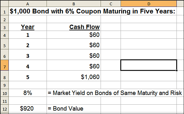
Exhibit 7-13. Using NPV to calculate the value of a bond
Bond prices always move in the opposite direction from interest rates. If you were to enter 5% in cell A10 of the spreadsheet in Exhibit 7-13, you would see that the bond value becomes $1,043. The bond would sell at a premium to its par value because in that scenario the locked-in 6% coupon rate was greater than the 5% available on comparable bonds. If you pay $1,043 to purchase the bond, you will receive only the $1,000 par value when it matures. That $43 loss will exactly offset the above market interest you earned, and you will net the same 5% yield to maturity available on comparable bonds.
Example of Using IRR to Decide Which Bonds to Purchase
Suppose the investment manager for your firm’s defined-benefit pension plan is choosing between two bonds of comparable maturity and riskiness. Both bonds have a $1,000 par value and an 8-year maturity. Bond A is selling at par with a 9% coupon. Bond B has only an 8% coupon but can be purchased for $879. Which bonds offers the higher yield to maturity? To determine this begin by typing the cash flows associated with each bond into the spreadsheet in Exhibit 7-14. You can then use Excel’s built-in internal rate of return function to calculate the yield on each bond. The formula in cell B15 is =IRR(B5:B13). The formula cell in C15 is =IRR(C5:C13). You see that the yield on Bond A is 9%. That’s no surprise because it is selling par and has a 9% coupon. Bond B had only a 7% coupon, but because you can purchase it at a deep discount, it actually offers a higher yield. Bond B with a 9.2% yield would be the better buy.
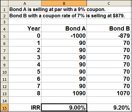
Exhibit 7-14. Using IRR to calculate the yield on a bond
Caution About the IRR Reinvestment Rate Assumption
The IRR criterion is extremely useful and widely used. Nevertheless, it has some potential weaknesses that you should understand. When comparing two projects, the one with the higher NPV will usually also have the higher IRR. There are however some situations in which that is not the case. The spreadsheet in Exhibit 7-15 calculates the IRR and NPV of Projects A and B. Project A has a higher IRR, but Project B has a higher NPV. That occurred because the IRR formula assumes the interim cash flows are reinvested at the same rate of return as the project that generated them. That assumption is too optimistic in situations in which the interim cash flows are reinvested at something closer to the firm’s weighted average cost of capital. In this example, Project A had larger cash flows in the early years and was therefore more affected by the high reinvestment rate assumption.
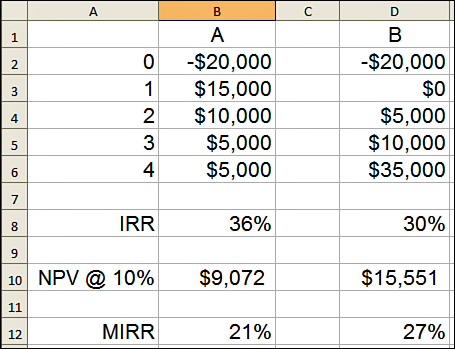
Exhibit 7-15. IRR and NPV do not always provide the same ranking.
Which project should you select when the NPV and IRR imply different rankings? You should base your choice on the NPV measures because there is no risk that they will be distorted by an unrealistically high unrealistic reinvestment rate assumption.1 An alternative would be to re-evaluate the projects using Excel’s MIRR function. The Excel formula for calculating this modified internal rate of return measure is
=MIRR(range, initial financing right, reinvestment rate)
This function enables you to specify the rate that will be earned by reinvesting the cash flows that are received prior to the project’s end. In Exhibit 7-15, the entries in cells B12 and D12 were =MIRR(B2:B6,10%,10%) and =MIRR(D2:D6,10%,10%). Project A had the larger IRR, but after entering a more realistic reinvestment rate assumption into the MIRR function, it is clear that Project B would be the better choice. As a practical matter, the capital budgeting spreadsheets illustrated in Chapter 9 include both NPV and IRR measures. This practice requires only a few extra keystrokes and will highlight any instances in which the NPV and IRR criterion might lead to different choices.
Why Decisions Should Not Be Based on Payback Periods
The payback period is usually defined as the original investment divided by the annual benefit. For example, if a new energy-efficient furnace costs $4,000 and then reduces fuel bills $800 per year, it would “pay for itself” in 5 years. The usual assumption is that the shorter the payback period, the more attractive the investment. Because they are easy to understand and easy to calculate, payback periods are often used in capital budgeting. Unfortunately, relying on payback periods can lead to a serious misallocation of resources. One problem with simple payback formulas is that they do not take into account the time value of money. This limitation can, of course, be overcome by calculating the number of periods it takes for the present value of future cash flows to just equal the initial investment. A more serious weakness in payback measures, even if based on discounted cash flows, is that they completely ignore the magnitude and duration of all benefits that occur after the payback period. Consider the two alternative projects described in Exhibit 7-16. Using the payback decision rule, you would prefer Project A because costs are recovered in 5 years instead of 7. In this case, that would be a bad choice. The NPV of Project B is $4.6 million, twice what this firm would earn on Project A. If you’re still not convinced of the limitations of payback models, consider that the option with the shortest payback period is always to do nothing at all. You might want to use payback periods as a tie-breaker if two projects are close in terms of projected NPV. That would be the equivalent of adopting a bird-in-hand philosophy assuming that the option with the shorter payback involves less risk. You should avoid, however, using payback periods instead of an NPV- or IRR-based decision model.
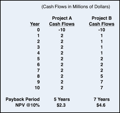
Exhibit 7-16. Payback periods can lead to the wrong decision.