
10. Equity-Based Compensation: Stock and Stock Options
During the 1980s, the pay packages of top executives were often unrelated to the success of the corporations they managed. How could that have occurred when their compensation consisted of salaries plus bonuses that were paid only if certain financial targets were achieved? In fact, CEOs received about 50% of their pay in the form of bonuses. The assumption was that the total compensation (salary plus bonus) received by these executives would be highly correlated with changes in company performance. The empirical data, however, failed to support that assumption. A frequently cited 1990 Harvard Business Review article by Michael C. Jensen and Kevin J. Murphy reported an extensive statistical analysis showing that annual changes in executive compensation did not reflect changes in corporate performance. Even though bonuses represented a large proportion of total compensation, Jensen and Murphy concluded that compensation for CEOs was “no more variable than compensation for hourly and salaried employees.”1 They and others argued for more aggressive pay-for-performance systems. Heeding this call, in the early 1990s corporate boards began to emphasize the creation of shareholder value. Equity compensation—that is, paying in stock and stock options—was seen as the most direct way to align shareholder interests and financial interests of managers. The use of equity compensation, particularly the granting of stock options, expanded dramatically during the 1990s. By 2003, 99% of large U.S. public corporations were granting stock options.2
How Do Stock Options Work?
Before looking at the specific characteristics of employee stock options, it may be helpful to review the use of exchange traded options. These are options publicly traded on a regulated exchange. These stock options are contracts that guarantee the option’s owner the right to either buy or sell the underlying stock at a specified price during a specified time period. The key point is that the option owner has the right, but not the obligation, to make this transaction. A call option provides the right to purchase a share of stock, that is, to call it in. A put option provides the right to sell a share of stock, that is, to put it to the other person. Now look first at a real estate analogy to see why one person might sell an option and another might purchase an option. Suppose you want to buy my house but only if your company transfers you to central New Jersey. We could sign a contract giving you the right to buy my home for a specified price, say $500,000, anytime during the next 12 months. That contract would require me to sell you my home if you decide to go forward with the deal but would not require you to purchase it if you chose not to. Why would I agree to take my home off the market for 12 months waiting for you to make a decision? I would do that only if you paid me some negotiated amount, say $10,000, to purchase that call option on my house. If you decided not to go through with the deal, I would keep your $10,000 and put my house back on the market. Stock options are similar in that the option purchasers pay for the right to make a transaction at a future date if they decide it is in their interest to do so. The option sellers receive a fee for agreeing to those terms. The amount paid to purchase an option is usually referred to as the premium.
What Is the Intrinsic Value of an Option? What’s the Time Value of an Option?
For a call option, the intrinsic value is the current stock price minus the exercise price. The exercise price is the price at which you have the right to exercise your option to purchase the stock. If a stock is currently selling for $45 and you have the right to buy it for $30, the intrinsic or minimum value of this option is $15. You could make a $15 profit by purchasing the stock at $30 and immediately reselling it at the current market price of $45. Why might the price of an option be greater than this minimum value? The possibility that the stock price could rise prior to the date the option expires makes its market value greater than its intrinsic value. If potential option buyers believe this stock’s price will rise above $45 before the option expires, they will be willing to pay more than $15 for the option. In fact, an option with an intrinsic value of zero (for example, the right to buy any time during the next year for $80 a share a stock that is currently selling for $80 a share) could have a market value well above zero. The portion of an option’s value attributable to the amount of time remaining before the option expires is referred to as the time value of that option.
Exchange Traded Options Are Sometimes Referred to as Listed Options
Exchange traded options are options traded on a regulated exchange that standardizes the contracts so that the underlying asset, quantity, expiration date, and strike price are known in advance. For example, Exhibit 10-1 shows the June 14, 2012, market price of call and put options on shares of Johnson & Johnson stock. On that date Johnson & Johnson stock was selling for $66.01 per share. The table shows the cost of purchasing call options with exercise prices (also called strike prices) ranging from $40 per share to $90 per share. For example, the market price of an option to purchase one share of J&J stock for $75.00 was $1.05. Why would anyone pay a $1.05 for the right to buy J&J stock at $75.00 when it was currently available for $66.01? You would buy that call option only if you believed that prior to the option’s expiration on the third Friday of June 2013, the J&J stock price would exceed $76.05 (the $75.00 you would pay for the stock plus the $1.05 you have already paid for the option). Suppose, for example, prior to the option’s expiration, the J&J stock price reaches $95.00. You could exercise your option to purchase the stock at $75.00 and then immediately resell it for $95.00. That $20.00 gain minus the $1.05 you paid for the option would leave you with a net profit of $18.95. If, on the other hand, on the day the option expired, the J&J stock price were below $75, you would let the option expire unexercised. There is an analogous case of buying a put option. You would pay $16 for the option to sell one share of J&J stock at $75 if you thought prior to the options expiration the J&J stock price would fall below $59 per share. If, for example, it fell to $40 per share, you could buy it at that price and then exercise your option to sell it at $75. Your profit would be $19 per share, the $35 per share gain minus the $16 you paid for the put option. You can profit from call options when the price of a stock goes up and from put options when the price of a stock goes down.
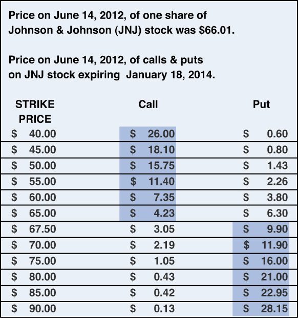
Exhibit 10-1. Example of exchange traded options
Source: http://investing.money.msn.com/investments/equity-options?symbol=us%3ajnj.
Are Options High-Risk Investments?
Are options high-risk investments? The answer to that question (and the answer to most questions) is, “It depends.” Naked options is the term used to describe trades in which the option purchaser does not also own shares of the underlying stock. Naked options can be extremely risky investments. Suppose the price of company X stock fell from $40 a share to $36 a share. If you had purchased $100,000 worth of stock when the price was at $40, you would have a 10% loss, but your investment would still be worth $90,000. What would your investment be worth if you had instead invested your $100,000 in options to buy company X stock at $40 per share? It would be worthless if on the day those options expired the stock price was $36. For the same movement in the stock price, the stock investment declined by 10% and the options investment declined by 100%. Covered options, on the other hand, can be a risk-reducing instrument. Covered options refer to trades in which the option buyer also owns shares of the underlying stock. Suppose you own 1,000 shares of Apple stock worth $700,000. You plan to retire in 1 year and are concerned that if the Apple stock price drops dramatically, your retirement will be much less comfortable. If you purchased for $8.00 each 1,000 put options giving you the option to sell 1,000 shares of Apple stock for $700 per share, you have limited your loss to $8,000. If the stock price fell to $350 per share but you have the right to sell your shares at $700, the $8,000 you paid for the put options prevented a $350,000 loss on the stock. You could think of that $8,000 as the cost of buying portfolio insurance. Of course, if the Apple stock price had risen by 10%, what would have been a $70,000 gain would be reduced by what you paid for the (unused) puts, and your net benefit would be only $62,000.
Options Trading Can Involve Many Different Strategies
Clever, but not always successful, traders have devised a large number of sometimes complex strategies for using options. These have colorful names such as Guts, Butterfly, Straddle, Strangle, Risk reversal, Bull put spreads, and on and on. You don’t need to understand any of those to design and manage employee stock option programs. However, illustrating one simple one may provide some insight into how calls and puts can be pieced together. A strategy referred to as a straddle involves buying a put and a call on the same stock. Suppose Boeing and Airbus compete for a large jetliner contract. You don’t have an opinion about which firm will win the contract, but you do believe that as soon as the winner is announced, the price of Boeing stock will soar if Boeing wins the contract or plummet if Boeing loses the contract. If Boeing stock price is currently selling for $75 per share, you could bet on that anticipated volatility by simultaneously buying calls giving you the right to purchase Boeing stock at $75 and puts giving you the right to sell Boeing stock at $75 a share. If the calls cost you, for example, $3 each and the puts $2 each, you have invested $5 per share to create this trade. If the stock moves up by more than $5, you exercise the call and make a profit. If the stock price falls by more than $5, you exercise the put and make a profit. Using straddles you can make money whether a stock price rises or falls, as long as the movement in one direction or the other is large enough.
How Do Employee Stock Options Differ from Exchange Traded Options?
Employee stock options cannot be bought or sold on public stock exchanges. Employers grant them, usually at no cost, to senior executives and sometimes also to non-executive employees. Employee stock options give the employee the right purchase shares of the employing company’s stock at a specific price during a fixed time period. Suppose for example, the company’s stock is currently selling for $50 a share and the employee is granted the right to purchase 1,000 shares at today’s price any time in the next 10 years. If 6 years from now, the stock is selling for $80 a share and the employee exercises her option to buy 1,000 shares at $50 each, she will have an immediate gain of $30,000 ( (80 – 50) × 1000). The hope is that the prospect of such gains will create an incentive for employees to behave in ways that will make the firm more successful and cause the stock price to rise faster. Employee stock options are by definition call options because they provide the right to purchase shares of stock. Employee stock options differ from exchange traded options in a number of important ways:
• They are granted or given to employees, so there is no purchase price.
• They are usually nontransferable; that is, they cannot be sold prior to exercise.
• They often have a vesting period, that is, the options are forfeited if the employee does not stay with that firm for a specified period of time.
• They tend to have longer exercise periods than exchange traded options. The average life of employee stock options is often 7 to 10 years. The exercise period for exchange traded options is typically months or at most a year or two.
As will be discussed next, these differences mean that the market price of exchange traded options is not usually a good proxy for the value of employee stock options.
Equity Compensation Can Be Options, Shares, or Both
The graph in Exhibit 10-2 is based on data reported by Frederic W. Cook and Company, Inc.,3 a large consulting firm specializing in executive compensation. This firm conducts an annual survey of the executive compensation practices of the 250 largest U.S. companies in the Standard & Poor’s 500 index. The trends shown in this graph are quite dramatic. In 2003, 99% of these large firms granted stock options to their senior executives. By 2011, the percentage granting options had declined to 70%. During the same period the proportion of firms offering their employees performance shares increased from 26% to 72%. Performance shares are shares of company stock given to managers only if certain companywide performance targets, such as an increase in revenues or earnings-per-share, are reached. The percentage of firms granting stock options may continue to decline, but for the foreseeable future, it is likely that options will continue to be used by the majority of large firms. Stock options are increasingly granted in combination with outright share grants or share grants contingent upon company performance. Possible explanations for the decreasing reliance on employee stock options are discussed in the following sections.
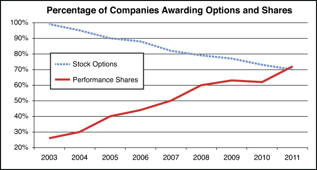
Exhibit 10-2. Trends in equity compensation
Source: Graph prepared with data extracted from the following reports released by Frederic W. Cook & Co., Inc.: The 2004 Top 250, September 2004, page 4. The 2008 Top 250, October 2008, page 5. The 2011 Top 250, October 2011, page 7.
Do Employees Prefer Options or Stock?
What are the key differences between paying in options and paying in shares of stock? If given the choice would employees prefer to receive options or shares? To explore these questions use the specific example described in Exhibit 10-3. The assumptions are that a company whose stock price is currently $40 per share is considering two alternatives. This firm will give employees either A) 1,000 shares of company stock or B) options to buy 8,000 shares of stock at today’s $40 price any time during the next 10 years. These employee stock options are valued at $5 each. Is it more expensive to grant stock or options? As this example illustrates there need not be any cost difference. By adjusting either the number of shares or the number of options, it is straightforward to define two alternatives that would have the same cost to the company. If the cost is the same, how would you choose between these alternatives? That choice should not be left to the firm’s finance department but should be based on the HR department’s assessment of which alternative would have the most beneficial incentive effects. To begin that analysis look at the impact a $20 change in the stock price would have on stockholders and on option holders.
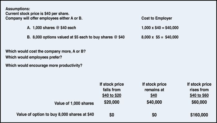
Exhibit 10-3. Does a $40 change in stock have the same impact on stockholders and option holders?
Employees Granted Shares Benefit Even When the Stock Price Goes Down
This example reveals clearly that paying with options is a highly leveraged form of compensation. If the stock price is still $40 at the time the options expire, the value of the 8,000 options will be zero. Had employees received 1,000 shares instead of options and the stock price remained at $40, their equity compensation would be worth $40,000. That’s a big difference. If the stock price doesn’t change or falls, employees benefit substantially more from a grant of shares than from a grant of options. The situation reverses, however, if the stock price rises. If on the day the options expire the stock price is $60, the employee’s 8,000 options will be worth $160,000 ( [$60 – $40] × 8,000). The value of 1,000 shares on that date would be $60,000. That’s $100,000 less than the value of 8,000 options.
Do All Employees Have the Same Risk Preferences?
Which alternative would employees prefer, and which alternative would create the stronger incentive effects?
The answer to those questions depends upon the personalities of the employees involved and their positions in your organization. Risk-averse employees would probably prefer to receive shares instead of options. For them it may be important to know that their equity compensation will be worth something even if share prices remain flat or decline. Regardless of personal risk preferences, employees at lower income levels may prefer shares because they would be less able to adjust their personal finances to accommodate large fluctuations in the value of their equity compensation. Less risk-averse employees and employees at higher income levels will probably prefer to receive a larger percentage of their compensation as options. These employees may be willing to accept some additional risk to have the possibility of a much larger payout. In the previous numerical illustration, at a stock price of $60 per share, the option holders received a payout of $160,000 compared to the $60,000 benefit they would’ve gotten from 1,000 shares. That’s a $100,000 difference for the same movement in stock price. The difference gets even bigger as the share price continues to climb. At $85 per share 1,000 shares would be worth $85,000, whereas 8,000 options would be worth $360,000 ([$85 – $40] × 8000). At that the price level, the difference is $275,000!
The finance department can calculate the cost differences, but the HR department should be assessing which combinations of stock and options are more likely to motivate and retain key employees. The mix preferred by employees is not necessarily the mix corporations will prefer. HR managers must determine whether increasing the amount of at-risk pay is a desirable compensation strategy in each of the specific situations they encounter. Risk-averse employees might prefer cash over either stock or options, but that would not create the wanted incentive effects. Risk tolerant executives might prefer options over stock. Would a highly leveraged compensation package like that optimize executive incentives to increase performance, or would it encourage them to swing for the fences and expose the firm to unwarranted risk? These are not easy questions to answer, and the analysis of these behavioral issues should not be left to the finance department. For HR managers to participate in that discussion, they must understand the financial and accounting aspects of options so they can make judgments about how employees will respond. The data in Exhibit 10-2 shows a significant and consistent decline in the granting of stock options. What triggered this decline? Part of the explanation may be that firms concluded that the overuse of employee stock options was encouraging excessive risk-taking. That is, however, not the primary reason. The primary reason for this change in compensation practices was a change in accounting practices.
The Debate over the Expensing of Stock Options
The Financial Accounting Standards Board (FASB) in 2004 altered the existing generally accepted accounting principles to require for the first time that employee stock options had to be expensed in the year they are issued.4 Prior to that time a company could choose to either include or not include the cost of employee stock options along with the other expenses shown on its income statement. If it chose not to recognize the cost of employee stock options on its income statement, it was required to show only in a footnote how large that expense would have been had it been included in its income statement. Sound like a strange rule? It was. Only a handful of major companies (for example, Coca-Cola, General Electric, Wachovia Bank, Bank One, and the Washington Post) chose to subtract the cost of employee stock options on their income statement.5 Companies were reluctant to expense options because doing so would lower their reported net income and earnings per share. Of course, where on the page you chose to show that expense affects only the reported net income, not the actual business reality. The decision to expense or not expense options sometimes had a substantial effect on a firm’s reported bottom line. One study by Merrill Lynch estimated that by not expensing options, companies in the Standard & Poor’s 500 index overstated their earnings by 10%.6
The FASB decision followed years of debate during which much of corporate America argued that the expensing of options was not necessary because option grants were not a business expense but merely the transfer of an ownership interest from one group of individuals to another, that is, from current stockholders to employees. If that argument had prevailed, it would have implied that paying in stock was also a nonexpense because it is also just a transfer of an ownership interest from current stockholders to employees. Direct stock grants have always been treated as a compensation expense, and there were no serious proposals to change that practice. The argument for expensing options is that if these equity instruments were not given to employees, they could be sold the public. The price the public would have paid for these options is the opportunity cost of giving them to a firm’s employees. Berkshire Hathaway CEO Warren Buffett summarized the case for expensing option well when he asked, “If stock options aren’t a form of compensation, what are they? If compensation isn’t an expense, what is it? And, if expenses shouldn’t go into the calculation of earnings, where in the world do they go?”7
Changes in the Accounting Treatment of Options Does Not Change Their True Cost
Now that the expensing of employee stock options is mandatory, firms are reducing the number of options granted. In 2003, 99% of large firms granted options to their top executives. The expensing of options became mandatory in 2004, and as was shown in Exhibit 10-2, the percentage of large firms granting options declined in that year and each subsequent year. By 2011, that percentage was down to 72%. Was this a rational response to the changing accounting rules? There are legitimate reasons to be concerned about the precision of the approaches used to estimate the cost of the employee stock options. Nevertheless, whatever the true cost of granting options is, the change in the accounting rules did not increase that true cost by one cent. If the accounting rules didn’t increase the true cost of options, why are fewer firms using them? It seems that the extensive use of options prior to 2004 was not driven by judgments about the optimal compensation strategy but by the desire to maximize reported earnings. Speaking in 1998, Warren Buffet observed, “Accounting principles offer management a choice: Pay employees in one form and count the cost, or pay them in another form and ignore the cost. Small wonder then that the use of options has mushroomed.”8 This emphasis on reported, as opposed to true, earnings was obviously not in the best long-run interest of shareholders. Now that both option grants and stock grants must be expensed, the playing field has been leveled. Firms can now choose the mix of option and stock grants that they believe will create value for shareholders without having this decision distorted by the accounting rules.
Using Black-Scholes to Estimate the Cost of the Options Granted
Now that options expensing is mandatory, firms are paying greater attention to the methodologies used to calculate the dollar cost of option grants to their employees. The choice of methodology can have a direct effect on the firm’s bottom line. The price of exchange traded options is set by the marketplace. It is determined by what buyers are willing to pay and what sellers are willing to accept. Because employee stock options usually differ from exchange traded options in a number of significant ways, the price of options traded in the marketplace is not a useful proxy for the value of options granted to employees. Most firms must rely on financial models to estimate the cost of their employee stock options. The most widely used of these is the Black-Scholes model,9 named for Fisher Black and Myron Scholes, the two Nobel prize-winning economists who developed it. However, over the last few years, a significant number of firms have shifted to alternatives such as lattice models or Monte Carlo simulations. These alternatives are discussed next. Decisions about which model to use should not be left to the finance department. An understanding of employee behavior is required when choosing among alternative models, and the choice of model may influence future compensation strategy decisions. HR managers should be active contributors to these discussions.
The equations underlying the Black-Scholes model are complex, but HR managers without a mathematics background can still achieve a good intuitive understanding of what the model does and how they can use it to design and manage employee stock option programs. The Black-Scholes value of an option can be calculated by plugging a few numbers into a spreadsheet of the type described next. The Black-Scholes model estimates the present value of the expected payoff an employee will receive from an options grant. The logic and calculation of present values is discussed in Chapter 7, “Capital Budgeting and Discounted Cash Flow Analysis.” The expected payoff is just the average payoff that an individual would receive if she purchased (or was granted) an option with these characteristics on many occasions. If you go to a casino and play a game where there is a 30% chance of winning $50 and a 70% chance of losing $25, the expected payoff is –$2.50 (.30 × $50 + .70 × –$25). If you played that game 1,000 times, your average outcome would be close to a loss of $2.50 per play. That expected payoff was calculated by multiplying each of the possible outcomes by the probability that outcome would occur and then summing those products. As you see next, the Black-Scholes model estimates all the possible payoffs from an option and the probability that each of those payoffs will occur. It then uses that information to calculate an expected payoff and expresses that expected payoff in present value terms.
The Black-Scholes model estimates the range of potential payoffs to an option by assuming that on average the price of the underlying stock will increase at the risk-free interest rate. The risk-free interest rate is the rate you could earn on a riskless investment such as U.S. government bonds. This assumption is illustrated in Exhibit 10-4. If the annual risk-free interest rate is 5%, the assumption is that stocks that trade at $38 a share at the beginning of the year will on average trade at $40 ($38 × 1.05) at year’s end. Of course, that number is only an average. Roughly one-half the time, the price will be greater than $40 and roughly one-half the time less than $40. The distribution of possible stock prices around the expectation of $40 is represented by the curve in Exhibit 10-4. The specific shape of the curve assumed by the Black-Scholes is a lognormal distribution. This is just a variation on the normal or bell-shaped curve that you may be familiar with. Important characteristics of lognormal distributions are that they do not include values below zero and are skewed to the right. That makes sense because a stock’s price can never fall below zero and has no fixed limit on the upside. The distribution is skewed to the right because a stock’s price can drop only 100% but can rise by more than 100%. Because the distribution is skewed to the right, the mean of the distribution ($40) is slightly to the right of the dotted vertical line.
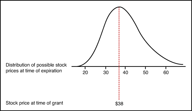
Exhibit 10-4. Log-normal curve to describe distribution of possible future stock prices
Stock prices slightly above or slightly below the mean are assumed to be more likely to occur than prices far above or far below the mean. In this example, stock prices between $40 a share and $50 a share are more likely to occur than prices between $50 and $60. Prices between $50 and $60 a share are more likely than prices between $60 and $70. Prices above $70 (or below $20) are possible but have an even lower likelihood of occurring. How rapidly the probability of occurrence drops off as the price deviates from the mean is determined by what statisticians call the standard deviation of the distribution. Roughly speaking the standard deviation is just the average deviation around the mean stock price. In this example, a low standard deviation would mean prices cluster tightly around the expected value of $40. A large standard deviation would mean prices are spread out over a much larger range. The simplest way to calculate the standard deviation in a stock’s price is to use past history. Some analysts, however, prefer to use an estimate of what future price volatility will be. After you have an estimate of the mean stock price and standard deviation of the distribution, you can use the known properties of the lognormal distribution to calculate the probability of each possible stock price occurring. In Exhibit 10-4 that probability is shown graphically as the height of the curve at each stock price.
You can then convert your estimate of the distribution of possible stock prices at the time of exercise into an estimate of the distribution of possible option payoffs. For example, if the exercise price is $38 and the stock price at expiration is $50, the value of the option is $12 ($50 – $38). And analogous calculation could be done for all possible stock prices. Of course, for all stock prices below the exercise price of $38, the value of the option will be zero. There is no value to having the right to buy something at $38 that is selling in the public marketplace for less than that. Weighting each of these possible payoffs by the probability that it will occur, you can calculate the average payoff you would receive if you purchased an option like this many times. That average or expected payoff, when expressed in present value terms, is the value to the employee and the cost to the employer of this option grant. The cost per option would then be multiplied by the number of options granted to determine the total cost.
Understanding the Inputs to the Black-Scholes Model
The original Black-Scholes model did not take dividends into consideration. An extension of the original model proposed by Robert Merton in 197310 does incorporate the impact on option prices of dividend payments. It is this version that is most often used to price employee stock options. Fortunately, you do not need to master or even understand the Black-Scholes-Merton equations shown in Exhibit 10-5 to effectively use this model. Most corporations purchase commercial software to do these calculations on a large scale, but a quick Internet search would reveal numerous, free online calculators for determining the Black-Scholes value of a stock option. If you are willing to do a little typing, you can easily create your own Black-Scholes spreadsheet by following the model shown in Exhibit 10-6. The inputs describing the option are entered on Row 3. To calculate the Black-Scholes value based on these inputs, type in the following formulas:
in cell B6: =(LN(B3/C3)+(D3-G3+F3^2/2)*E3)/
(F3*SQRT(E3))
in cell C6: =B6-F3*SQRT(E3)
in cell D6: =NORMSDIST(B6)
in cell D8: =D6*B3*EXP(-G3*E3)-E6*C3*EXP(-D3*E3)
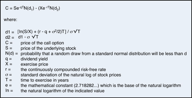
Exhibit 10-5. Black-Scholes-Merton option pricing formula
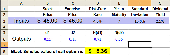
Exhibit 10-6. Spreadsheet for calculating Black-Scholes value on an employee stock option
The six inputs to this model are
• Current stock price
• Price at which the option can be exercised
• Risk-free interest rate
• Years to maturity or expected life of the option
• Standard deviation in the price of the underlying stock
• Dividend yield on the underlying stock.
By adjusting each of these inputs up and down in the previous spreadsheet, you can quickly see the impact they have on the estimate of the options value. If you understand what makes an option valuable, you should not be surprised which changes increase the option’s value and which lower it.
• Stock price and exercise price: The value of the option increases when the amount by which the current stock price exceeds the exercise price increases. The right to buy shares at $45 is more valuable when the current stock price is $65 than when the current stock price is $55. Employee stock options are typically granted with an exercise price equal to the current stock price. Their value depends upon how much the company’s stock prices will rise in the future.
• Risk-free interest rate: The value of an option increases when the interest rate increases. One benefit of an option is that you get to hold onto your money until the option is exercised. If you buy 1,000 shares today at $45, you must immediately pay out $45,000. If you have the option to buy those same shares at the same price 7 years from now, you get to hold onto your $45,000 for an extra 7 years. The benefit from holding onto your $45,000 for 7 years depends on interest rates. The higher the interest rate, the more you can earn on your money during that 7-year period.
• Years to maturity: The value of an option increases when the years to maturity or the expected life of the option increases. Options have value for two reasons. They enable you to wait to see what happens to the stock price before making a decision about whether to purchase shares, and they enable you to hold onto your money until the option is exercised. Both of those benefits increase as the length of the option increases. With longer options, there is more time for the share prices to grow, and you get to retain your cash for a longer period.
• Volatility of the stock price: The value of an option increases when the volatility in the price of the underlying stock increases. Volatility is measured as the standard deviation in annual stock price changes expressed as percentage. A large standard deviation means there are large swings in the price of that stock. A lower standard deviation would mean the price fluctuations remain within a narrower range. For stock owners, higher price volatility means a greater chance of big gains and a greater chance of big losses. For option holders higher volatility means a greater chance of big gains, but not a greater chance of big losses. The value of an option increases as the stock price rises further above the exercise price. However, the value of an option does not change as the stock price falls further below the exercise price. The option value is zero whether on the date of expiration the stock price is $10 below the exercise price or $100 below the exercise price. Option holders benefit from greater volatility because it means a chance for bigger gains without exposure to the possibility of greater losses. The Black-Scholes value of an option is often more sensitive to changes in the volatility estimate than it is to changes in the other inputs to the model. In Exhibit 10-6, if you change only the volatility estimate from 15% to 25%, the value of the option rises from $8.36 to $11.81.
• Dividend yield: The value of an option decreases when the dividend yield on the underlying stock increases. The dividend yield is measured as the annual dividend paid divided by the average stock price in that year. What happens to the profits earned by the corporation during the period between the time the option is granted and the time it is exercised? Like all profits, they will either be distributed as dividends or retained in the corporation. If they are distributed as dividends, this value goes to current stockholders, not to the option holders. This will, other things equal, decrease the value of the shares the employee will in the future have the option to purchase. Simply put, option holders would prefer the company not distribute any dividends until they exercise their options and become shareholders.
• Vesting periods and forfeiture rates: The cost to the firm to grant employees stock options declines when the forfeiture rates increase. Employees who do not stay with the firm for the full vesting period often forfeit their right to these options. These factors are not inputs to the Black-Scholes model but can be used to adjust the results coming out of that model. For example, if the firm granting the options described in Exhibit 10-6 had a 2-year vesting period and a 5% employee exit rate, the value of the option would be $7.55 ($8.36 × .95 ×.95).
The Input Not Used by the Black-Scholes Model
It may seem counterintuitive, but expectations about whether the price of this stock will rise or fall are not an input to the Black-Scholes model or any other option costing model. Because options can be used to bet on a stock going up or down, the assumption is that the risk associated with any option could be exactly offset by creating a second portfolio whose value moved in the opposite direction. This ability to hedge away all risk allows options to be priced on a risk-neutral basis, that is, without any assumption about the direction of future movements in the stock price. It also allows options to be valued by assuming that the expected return on the underlying stock will equal the risk-free rate interest rate.
Firms Must Disclose the Methods and the Assumptions They Use to Cost Stock Options
The Financial Accounting Standards Board’s Accounting Standards Codification 718 on Stock Compensation (ASC 718) requires that all equity compensation be expensed at “fair value.” For awards such as restricted stock and performance shares, fair value is the current value of the stock. For stock options and stock appreciation rights, fair value is estimated using an option-pricing model such as Black-Scholes. For stock options that vest over time the compensation expense is recognized over that vesting period. ASC 718 also requires that in the footnotes to its financial statements a firm disclose information describing the nature and terms of its share-based payments, the method of estimating fair value, and the effect of these compensation costs on the income and cash flow statements. The list of specifics that must be disclosed is extensive. Exhibits 10-7 and 10-8 contain only excerpts from the stock option footnotes in the 2011 annual reports of Johnson & Johnson and Alcoa.
The fair value of each option award was estimated on the date of grant using the Black-Scholes option valuation model that uses the assumptions noted in the following table. Expected volatility represents a blended rate of 4-year daily historical average volatility rate and a 5-week average implied volatility rate based on at-the-money traded Johnson & Johnson options with a life of 2 years. Historical data is used to determine the expected life of the option. The risk-free rate was based on the U.S. Treasury yield curve in effect at the time of grant.
The average fair value of options granted was $7.47, $8.03, and $8.35, in 2011, 2010, and 2009, respectively. The fair value was estimated based on the weighted average assumptions of
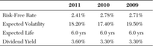
Exhibit 10-7. Excerpt from the 2011 stock option footnotes of Johnson & Johnson
Source: Johnson & Johnson 2011Annual Report, page 54.
The fair value of new options is estimated on the date of grant using a lattice-pricing model with the following assumptions:
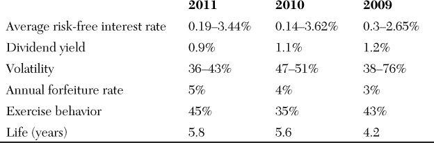
The exercise behavior assumption represents a weighted average exercise ratio (exercise patterns for grants issued over the number of years in the contractual option term) of an option’s intrinsic value resulting from historical employee exercise behavior. The life of an option is an output of the lattice-pricing model based upon the other assumptions used in the determination of the fair value.
Exhibit 10-8. Excerpt from the 2011 stock option footnotes of Alcoa
Source: Alcoa 2011 Annual Report, page 126.
J&J Used Black-Scholes to Price Employee Stock Options
The interpretation of the information in the Johnson & Johnson footnote is relatively straightforward. J&J’s Black-Scholes model uses a risk-free interest rate of 2.41% based on U.S. Treasury bonds. J&J says that its historical experiences have been that employees exercise their options on average after about 6 years. In 2011, J&J stock paid dividends equal to 3.6% of the average stock price. The one assumption that may warrant some explanation is the expected volatility in the price of J&J stock. J&J reports that it was estimated using a combination of historical data and the implied volatility from exchange traded options on J&J stock. To find the volatility implied by the market price of J&J’s exchange traded options, you can plug into the Black-Scholes formula the market price of those options and all the Black-Scholes variables other than volatility. Then solving algebraically for volatility, you can obtain an estimate of what the market on average was assuming about how much variability there will in the future prices of J&J stock. The disadvantage of using historical volatilities is that history may not repeat itself. The disadvantage of using implied volatilities is that they are only estimates of what may happen in the future. J&J chose to use a blend of the two.
Alcoa Used a Lattice Model to Price Employee Stock Options
The footnote excerpted in Exhibit 10-8 shows that Alcoa used a lattice pricing model instead of Black-Scholes. Models such as the one illustrated in Exhibit 10-9 are often referred to as lattice models because of their lattice-like appearance. Before discussing why an increasing number of firms are shifting to lattice models, it is probably useful to review how these models work. Like the Black-Scholes models, lattice models estimate the present value of the expected payoff an employee will receive from an options grant. As in Black-Scholes, that expected payoff is calculated by multiplying each of the possible outcomes by the probability that outcome will occur and then summing those products. The difference is that in the Black-Scholes model the distribution of possible stock prices at the time of expiration is described by a continuous distribution, the lognormal curve discussed in the previous section. Under the lattice model, distribution of possible stock prices is represented by a range of discrete price points.
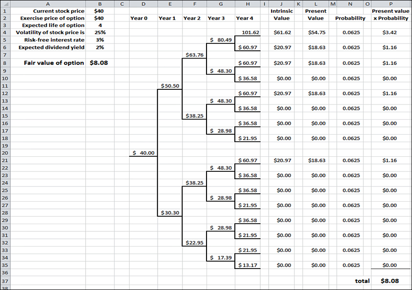
Exhibit 10-9. Example of a simplified binomial options pricing model
Most lattice models assume that the price of the underlying stock will follow a binomial distribution, a type of probability distribution in which the underlying event has only one of two possible outcomes. These models break down the time to expiration into a series of discrete intervals, or steps. The assumption is that at each step the stock price will either increase by a specific amount or decrease by a specific amount. The simplified binomial model in Exhibit 10-9 assumes that the term of the option is 4 years and that each step equals 1 year. Therefore, at the end of year 1, there are only two possible stock prices. The year 2 stock price is dependent upon where the price ended year 1. As you can see in the diagram, this process means there are 4 possible prices at the end of year 2, 8 possible prices at the end of year 3, and 16 possible prices at the end of year 4. Had this model been extended out to the 10-year term of a typical employee stock option, the number of price possibilities at the end of the last year would be more than 1,000. Using this estimate of the distribution of possible stock prices at the time of expiration, you can calculate the expected payoff to the option holder.
If You Want to Know How the Spreadsheet Was Calculated
This simplified binomial model (see Exhibit 10-9) assumes the stock price in each period will grow at the risk-free interest rate minus the dividend rate. The price will then be that amount plus one standard deviation or that amount minus one standard deviation. The formula in cell E11 is =D20*(1+B5-B6)*(1+B4). The formula in cell E28 is =D20*(1+$B$5-$B$6)*(1-$B$4). Analogous formulas were entered into columns F, G, and H. The intrinsic value of the option, the amount of payoff that would be received at each price level, is shown in Column J. That amount is just the stock price minus the exercise price of $40 per share. Because those gains would be received 4 years from now, they need to be converted into present values. That calculation is done in Column L by dividing the intrinsic value from Column J by (1+i)t. The formula in cell L4 is =+J4/(1+B5)^4. Column N shows the probability that each of those values will occur because there are 16 equally likely outcomes that probability is 1.0/16, which is .0625. The present values from Column L are multiplied by these probabilities, and the product is shown in Column P. The values in Column P are then summed in cell P37. The value in cell P37 is the weighted average of the possible outcomes that is the expected payoff from the option.
Why Do Some Firms Prefer Lattice Models over Black-Scholes?
The Black-Scholes model is easy to calculate. You enter the assumptions into a single equation and obtain an estimate of the option’s value. However, the Black-Scholes model assumes the value of the input variables (volatility, interest-rate, and dividend yield) are fixed over the term of the option. That’s not always the case. More important, it also assumes there is no early exercise, that is, that all employees will hold their options until the expiration date. That assumption is seldom, if ever, true. In practice, firms attempt to incorporate early exercise behavior into the Black-Scholes model by using the average number of years before exercise, rather than the maximum term of the option as the input assumption. Because the Black-Scholes assumptions are seldom perfectly satisfied, the results obtained with that model are at least open to question.
The lattice model is more cumbersome to calculate because you must specify perhaps hundreds of steps in a binomial tree. However, an advantage of the lattice model is that at each step, you can use different volatility, interest-rate, and dividend yield assumptions. The biggest advantage of the lattice model is that you can explicitly model early exercise behavior, and if you want you can model the exercise behavior differently for different groups of employees. The basics of modeling the early exercise are illustrated in Exhibit 10-10. In this example, you do not assume that all employees will hold their options until they expire at the end of 4 years. Instead, assume that employees will exercise their options if and when the current stock price reaches a level equal to or greater than 150% of the exercise price. In other words, the assumption is that when the reward from exercising gets large enough, employees will grab the bird-in-hand rather than continue to hold their options and expose themselves to the possibility that the stock price will fall. In Exhibit 10-10, one of the four possible stock prices at the end of year 2 satisfied this condition ($63.76 > (1.50 × $40). There is a 25% chance that the $63.76 price will be reached the end of year 2. If that happens the model assumes the option will be exercised at that point. The distribution of possible payoff values is adjusted and the expected payoff recalculated. In this example, explicitly modeling early exercise behavior reduced the option value to $7.93 from the $8.08 shown in Exhibit 10-9. The effect would have been larger if the example extended the binomial tree out to the 10-year term of a typical employee stock option. The effect would have also been larger if you assumed that less than a 50% increase in the stock price was required to trigger early exercise. The footnote shown in Exhibit 10-8 indicates that the Alcoa lattice model assumed early exercise would occur when the stock price grew by 45%.
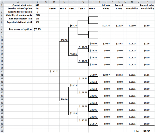
Exhibit 10-10. Assumes early exercise will occur when stock price reaches 150% of the exercise price
To summarize, lattice models enable the firm to build in assumptions about when early exercise will occur. If options are exercised prior to the expiration date, that changes the distribution of possible option payoffs. Changes in that distribution alter the average benefit employees receive from these options. That expected benefit is the value of the option used in the calculation of the firm’s employee stock option expense. If the choice of the options pricing model affects the estimated value of the options, it also affects the expense shown on the income statement and the bottom-line net income that the company reports.
The lattice models in Exhibits 10-9 and 10-10 are simplifications created to illustrate the basic logic behind these approaches. In practice, the lattice model most often used to value employee stock options is the Hull-White model.11 An example of the type of lattice models that can be designed following the Hull-White approach is shown in Exhibit 10-11. The simplified examples in Exhibits 10-9 and 10-10 were four-step binomial models. The example in Exhibit 10-11 is a 200-step trinomial model. A binomial model assumes there are two possible price outcomes at each step, an increase or a decrease. A trinomial model assumes there are three possible outcomes. The price will increase, stay the same, or decrease. A 200-step model is one that divides the time between the grant date and the expiration date into 200 periods.
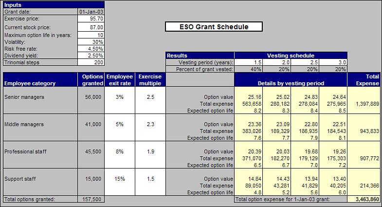
Exhibit 10-11. Worksheet from commercially available employee stock option software
Source: Hoadley Trading & Investment Tools website, http://www.hoadley.net/options/develtoolseso.htm, downloaded 8/24/2012.
The Black-Scholes model assumes a continuous distribution of possible stock prices. This distribution is illustrated by the curve in Exhibit 10-4. Lattice models assume a process that produces a distribution of discrete stock prices. This distribution is illustrated by the prices in Column H of the spreadsheet in Exhibit 10-9. However, as the number of steps in a lattice model increases, this distribution of discrete prices becomes a closer and closer approximation to the continuous distribution assumed by Black-Scholes. Using the same assumptions about the option terms and the underlying stock, Black-Scholes and 200-step lattice models such as the one shown in Exhibit 10-11 would yield almost exactly the same estimate of the option’s value. Of course, the purpose of going to a lattice model is that it offers the flexibility to use different input assumptions. For each year, you could use a different estimate of the stock price volatility, the risk-free interest rate, and the dividend yield. The biggest difference is that with the lattice models, you can specifically model early exercise behavior and forfeitures due to employee exits. As illustrated in Exhibit 10-11, different assumptions can be specified for different employee groups. A firm’s historical experience might indicate that, for example, less highly paid employees tend to exercise their options when the stock price exceeds 150% of the exercise price, but senior executives tend to not exercise early unless the stock price reaches 250% of the exercise price. Unlike the Black-Scholes model where expected time to exercise was one of the input variables, a lattice models such as the one in Exhibit 10-11 calculates the average life of the options based on the assumptions about the exercise multiples and the anticipated movements in the stock price. The Alcoa note in Exhibit 10-8 points out that this is the case.
Using Monte Carlo Simulation to Determine the Value of Employee Stock Options
Most firms still use a Black-Scholes model to estimate the cost of employee stock options. A growing number of firms use either a binomial or trinomial lattice model. A smaller percentage uses a Monte Carlo simulation. Each of these approaches uses a different method to estimate the distribution of possible stock prices at the time of expiration. The Black-Scholes model relies on a single equation that assumes that these prices can be described by a continuous lognormal distribution. Lattice models assume this distribution can be approximated by a series of discrete price points generated through a multistep binomial or trinomial tree. Monte Carlo simulations are the least rigid in their assumptions. These models perform a large number of random trials and observe the price distribution that results. A different application of Monte Carlo simulations was illustrated and discussed in Chapter 9, “Financial Analysis of a Corporation’s Strategic Initiatives.” When used to evaluate options, Monte Carlo models begin with an equation for predicting the future price of the underlying stock. That equation, which is the same one underlying in the Black-Scholes model, assumes that stock prices follow a random walk. Each period the stock price moves randomly either up or down. The magnitude of that movement is determined by the standard deviation of the changes in stock price. Monte Carlo simulations use random draws from a standard normal distribution to generate a sequence of random stock price movements and then calculate the stock price that would result. Each time that process is repeated, it generates one possible value of the stock price at expiration. That process is then repeated many thousands of times. The average of all these price possibilities is then used to calculate the expected payoff from the option. That expected payoff is then expressed in present value terms.
Dilution, Overhang, and Run Rates
Your CFO may have legitimate concerns about managing overhang. Overhang is the aggregate of the equity awards currently outstanding plus those authorized but not yet granted, divided by the fully diluted number of shares outstanding. In other words, a measure of how many shares have been or may in the future be issued through the firm’s equity compensation programs. When the overhang is large, shareholders may become concerned the company’s compensation practices will result in an excessive dilution of their ownership interests. Motivated by that same concern, companies carefully monitor their run rate, a measure of the rate at which they are issuing the shares under their shareholder-approved equity compensation plan. The higher the run rate, the sooner management needs to go back to the shareholders seeking an authorization for an increase in the share pool. Overhang and dilution are important constraints on the design of equity compensation programs. They should not, however, drive the design of these programs. Stock prices are a function of earnings-per-share. The denominator in the EPS ratio is the number of shares outstanding. Other things equal, if equity compensation programs increase that denominator, EPS and the stock prices will decline. That is the dilution effect that may be a concern to shareholders. However, if equity compensation programs are effective, other things will not be equal. Net income in the numerator will rise by more than enough to offset the larger denominator and EPS and the stock price will rise. Some forms of equity bases pay (for example, stock appreciation rights, restricted stock units, and performance share units) do not result in any dilution all. A brief description of these instruments is provided in Exhibit 10-12.
Stock options: A stock option is a right to purchase employer stock at a fixed price during a specified period of time. An expense is charged based on the option’s fair value on the grant date. Fair value is estimated using a Black-Scholes, lattice, or Monte Carlo model.
Restricted stock: Restricted stock is employer stock granted to employees at no cost. It is subject to vesting requirements and transferability restrictions. An expense is charged equal to the number of shares granted multiplied by the grant date market value of the stock.
Restricted stock unit (RSU): Restricted stock units are not stock, but cash payments equal in value to one share of stock. Units do not represent any actual ownership interest and have no voting or dividend rights. The amount expensed is equal to the number of RSUs granted multiplied by the grant date fair market value of a share of company stock.
Stock appreciation rights (SAR): Stock appreciation rights provide the employee a payoff equal to the appreciation in a specified number of shares of employer stock. The SAR’s fair value on the grant date is estimated using a Black-Scholes, lattice, or Monte Carlo model.
SARs provide a payoff to the employee only if the stock price appreciates. RSUs provide a payoff to the employee even if the stock price is flat or declines.
Performance shares: Performance shares are employer stock provided to employees if company performance reaches target levels. For Performance shares contingent upon financial performance (for example, EBIT, EPS, and ROE) at the end of the performance period, the expense is adjusted to equal the value of the shares that actually vest. Performance shares contingent upon stock market performance (for example, stock price change or TSR) are usually valued using a lattice model or Monte Carlo simulation. Black-Scholes models cannot easily incorporate the performance contingencies.
Performance share unit (PSU): Performance units are not stock, but cash payments equal in value to one share of stock that are made to employees if specified financial performance or stock performance targets are achieved. For PSUs contingent upon financial performance at the end of the performance period, the expense is adjusted to equal the value of the cash actually paid. PSUs contingent upon stock market performance are usually valued using either a lattice model or Monte Carlo simulation. Black-Scholes models cannot easily incorporate the performance contingencies.
Exhibit 10-12. Alternative forms of equity compensation
Equity Compensation Is One Tool for Aligning Executive and Shareholder Interests
HR managers need more than the ability to read and interpret the employee stock option footnotes in their firm’s annual report. To effectively design and manage compensation programs, they must understand the financial characteristics of alternative forms of equity-based pay. In many companies employee stock options now represent a smaller percentage of total compensation. Options are still widely used but often combined with other forms of equity compensation. They are also often combined with cash bonuses tied to stock performance measures such as the total shareholder return. Stock-related measures are, however, only one tool for aligning executive and shareholder interests. The alternative is to replace or combine stock market-based measures with financial statement-based measures of the increase in shareholder value. A range of such measures is discussed in Chapter 12, “Creating Value and Rewarding Value Creation.” Both approaches have their own strengths and weaknesses.