Chapter 14. Isochore and Isopach Maps
Introduction
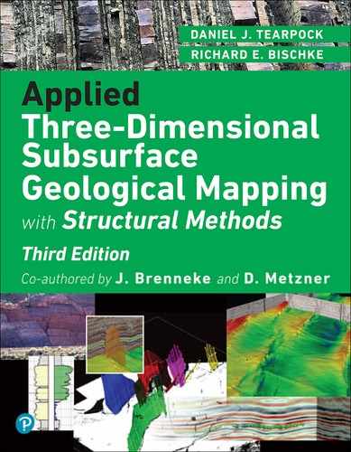
Two key terms, isochore and isopach, are often used synonymously in the petroleum industry as measures of thickness, but they are different. An isochore map (Fig. 14-1a) delineates the true vertical thickness of a stratigraphic interval, whereas an isopach map (Fig. 14-1b) illustrates the true stratigraphic thickness of a stratigraphic interval. These two terms are often confused with respect to their geological meaning. It is vital for both exploration and development work that the correct meaning and, more important, the correct application of these two thicknesses be understood.
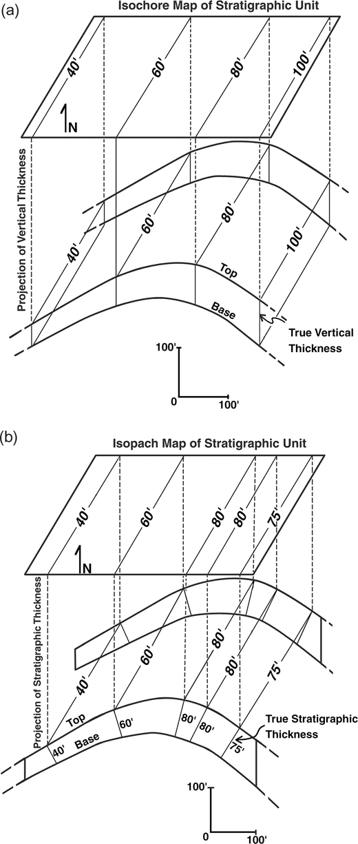
Figure 14-1 (a) An isochore map delineates the true vertical thickness of a stratigraphic interval, such as a rock unit containing a reservoir. (b) An isopach map delineates the true stratigraphic thickness of a stratigraphic interval. The same dipping stratigraphic unit is used in both (a) and (b), with the same edge-of-map boundaries. Note different thickness values assigned to the isochore map versus the isopach map of the same unit.
An isochored or isopached unit may be as small as an individual sand only a few feet thick or as large as several thousand feet thick and encompassing a number of stratigraphic units. An isopach map is extremely useful in determining the stratigraphic framework or the structural relationship responsible for a given type of sedimentation and for recognizing paleohigh areas. The shape of a basin, the position of the shoreline, areas of uplift, and under some circumstances the amount of vertical uplift and erosion can be recognized by mapping the variations in thickness of a given stratigraphic interval (Bishop 1960).
Isochore and isopach maps are used for a number of purposes by the petroleum geologist, including (1) depositional environment studies, (2) genetic sand studies, (3) growth history analyses, (4) depositional fairway studies, (5) derivative mapping, (6) the history of fault movement, and (7) calculation of hydrocarbon volumes.
In this chapter, we discuss several different types of isochore and isopach maps important to the evaluation of petroleum potential. These include interval isopach maps and net sand and net pay isochore maps. An interval isopach map delineates the true stratigraphic thickness of a specific unit or units. Interval isopach maps are discussed briefly near the end of this chapter.
An isochore map may be based on the total vertical thickness of a specific unit or based on an aggregate vertical thickness of a particular rock type within a stratigraphic unit. For example, a given unit may consist of interbedded permeable and impermeable strata. An isochore map can be made for the total unit consisting of both permeable and impermeable strata, or an isochore map can represent the aggregate vertical thickness of only the reservoir-quality rock within that stratigraphic unit. For simplicity and brevity in this chapter, we use the term net sand isochore map to refer to a map of only the reservoir-quality rock, although the term net reservoir isochore might be more precise. Therefore, a net sand isochore map represents the aggregate vertical thickness of reservoir-quality rock present in a particular stratigraphic interval, which is illustrated in Figure 14-2. The techniques and calculations to derive vertical thickness are explained in detail in this chapter. The fluid contained in a stratigraphic unit may be hydrocarbons or water, or any combination of the two. Figure 14-3 shows a net sand isochore map of the 10,500-ft Sand in Golden Meadow Field, Lafourche Parish, Louisiana, USA. A net pay isochore map delineates the aggregate vertical thickness of reservoir-quality rock that contains hydrocarbons (gas, oil, or both). An example is shown in Figure 14-5.

Figure 14-2 Net sand consists of porous reservoir-quality rock. All nonreservoir-quality rock is ignored. (From Tearpock and Harris 1987. Published by permission of Tenneco Oil Company.)
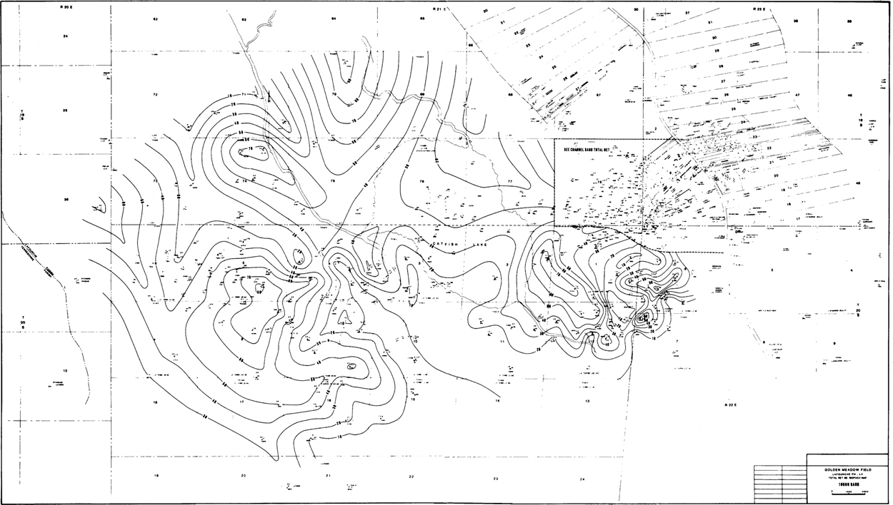
Figure 14-3 Portion of the net sand isochore map of the 10,500-ft Sand in Golden Meadow Field, Lafourche Parish, Louisiana, USA. (Published by permission of Texaco, USA.)
Net sand and net pay isochore maps of subsurface units are usually prepared from well log data, although seismic data may also be used. Interval isopach maps may also be constructed from well log data and seismic data, where coverage is adequate. As with structure maps, the completeness and accuracy of an isochore or isopach map depend on the amount and accuracy of data available. Even in isochore and isopach mapping, we cannot get away from the importance of log correlation work. Well log data, particularly correlations, should be studied very carefully in order to prepare an accurate and precise isochore map.
For volumetric reserve calculations, we are interested in obtaining the volume of a reservoir (solid material plus fluid-filled pore space). In this book, we use the volume unit acre-foot, which is standard practice in the United States. One acre-foot is equivalent to 1233.48 cubic meters and to 0.123348 hectare-meters. To many people, an acre-foot is an abstract measurement, but the concept is relatively simple. One acre-foot can be defined as that volume of rock plus fluid contained in an area one acre in size, with a thickness of one foot. How big is an acre? There is a very easy way for some people to visualize the size of an acre. One acre contains just about the same area as an American football field from goal line to goal line. A football field 300 ft long and 160 ft wide is equal to 48,000 sq ft, whereas one acre is equal to 43,560 sq ft. If we fill, with oil, a box that is one foot deep and the size of an American football field, the total volume of oil is just about equal to one acre-foot. In terms of barrels of oil, there are 7758 barrels (1233 cubic meters) of oil in one acre-foot. However, a reservoir volume of one acre-foot actually comprises solid material plus fluids that occupy the pore space. A calculation of oil-in-place in a reservoir must take into account pore space and water saturation as well as other factors. In creating a net pay map, we assume that within a net sand interval that contains hydro-carbons, all pore spaces are filled with hydrocarbons. The later calculation of hydrocarbons-in-place takes account of water saturation. In most cases, the structurally lower limit of a reservoir is a hydrocarbon/water contact, typically defined on the basis of parameters related to economic productivity, such as porosity and water saturation.
Sand–Shale Distribution
Most individual rock bodies do not consist exclusively of permeable rock; shale and other impermeable rock material are commonly distributed throughout the rock body as interbedded shale or impervious (tight) zones. The percentage and distribution of shale members or impervious zones varies widely within rock units. Net sand and net pay isochore maps are drawn on net effective sand (porous and permeable sand) only; therefore, shale and other nonreservoir-quality rock must be subtracted from the total interval to determine the net effective sand for isochore mapping.
In a given oil or gas well, the net effective sand to be used for isochore mapping is normally determined by computer analysis of digital log curves or detailed analysis of 5-in. well logs, supplemented by available core analysis. In Chapter 4, in the section Annotation and Documentation, we outline a method for annotating the percentage and distribution of net sand and impermeable layers that are present within a particular productive unit (Fig. 4-47). Once the net sand is determined for each well, a net sand map can be prepared for that sand. The aggregate of net sand for any particular well may contain water or hydrocarbons; net pay is that portion of the net sand that contains hydrocarbons in sufficient quantities to produce hydrocarbons at economic rates.
For a net sand or net pay map, the gross, or overall, interval to be mapped extends from the top of porosity to the base of porosity within the productive unit. Within that interval, the amounts of net sand and net pay vary with location. The net/gross ratio is the amount of net sand divided by the thickness of the gross interval, as determined from well logs and core analyses. The net/gross ratio within a productive unit can be mapped, based on log and core data, and used to estimate net sand and net pay at selected locations within the unit, as described later in this chapter.
Basic Construction of Isochore Maps
The procedure used in constructing an isochore map depends on whether the reservoir being mapped is a bottomwater or an edgewater reservoir. A bottomwater reservoir is a reservoir that is completely underlain by water (Fig. 14-4). An edgewater reservoir is one not completely underlain by water; some portion(s) of the productive unit is completely filled with hydrocarbons, and water underlies the remainder of the reservoir (Fig. 14-6).
Figure 14-4 Three-dimensional model of a bottomwater reservoir.
It is important to be able to visualize a hydrocarbon reservoir in three dimensions. Your ability to understand the configuration of a reservoir can affect the location of development wells, completion practices, and planned production.
Bottomwater Reservoir
Figure 14-4 is a 3D model of a bottomwater reservoir. This hydrocarbon accumulation, consisting of oil and gas, is trapped within an anticlinal structure. Notice how the oil and gas are segmented within the reservoir and completely underlain by water.
Figure 14-5 illustrates, in both map and cross-sectional views, a bottomwater oil reservoir. Looking at the cross section in the center of the figure, we can see the oil/water contact. The hydrocarbons are completely underlain by water; therefore, nowhere in the productive unit is there a full-thickness of oil. At any location within the reservoir, the amount of net pay equals the amount of net sand above the oil/water contact.
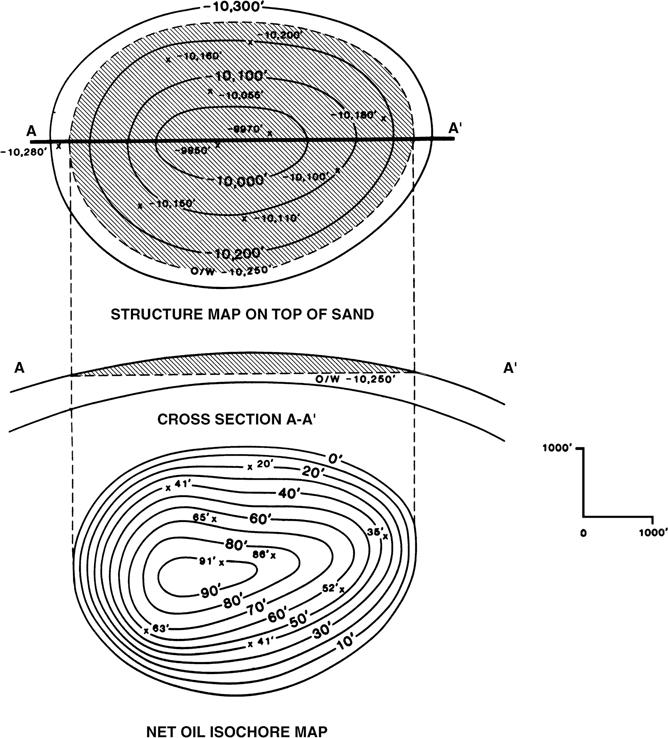
Figure 14-5 Structure map of the top of porosity, cross section, and net oil isochore map for a bottomwater reservoir. A net oil isochore map is a map showing the vertical aggregate thickness of reservoir-quality rock containing hydrocarbons. (From Tearpock and Harris 1987. Published by permission of Tenneco Oil Company.)
Net Pay Isochore Map Construction.
The construction of a net pay isochore map for a bottomwater reservoir requires a structure map on the top of porosity for a given productive unit, net pay values for each well in the reservoir, and the depth of the hydrocarbon/water contact. The following procedure is used to construct the net pay isochore map for a bottomwater reservoir (Fig. 14-5).
Post the net pay values for each well on a basemap. If deviated wells are included, the net pay values must be corrected to true vertical thickness.
Overlay the isochore basemap on the top-of-porosity structure map for the reservoir, and draw the outer limit of the hydrocarbon-bearing reservoir. The outer limit may be any boundary, or combination of boundaries, such as an oil/water contact, fault, pinchout, or permeability barrier. Where this outer limit of the productive reservoir area is a hydrocarbon/water contact, it becomes the zero contour line on the net pay isochore map, as shown in Figure 14-5. In this case, the outer limit of the reservoir is an oil/water contact at a depth of −10,250 ft. However, if a boundary of part of a reservoir is a more or less vertical surface, such as a vertical fault or a vertical salt face, then the amount of net pay adjacent to this surface will exceed zero.
Contour the net pay isochore map, which is contained within the area outlined by the zero line on the basemap. Be sure to honor all posted net pay values. The net pay contours may generally conform to the structure contours. Net pay contours are commonly drawn as being equally spaced. However, due to variations in net sand thickness within the reservoir, the isochore contours need not be equally spaced. Figure 14-5 is a net pay map of a reservoir in which the net oil contours reflect the structure in a general way, yet the contours are proportionally spaced due to variation in net sand within the productive unit. If the well control is limited, additional points of contour control may be obtained by using a method called walking wells or by using a net/gross ratio map, each of which allows us to estimate net pay at chosen points in a reservoir. These methods are explained in detail later in this chapter.
Always indicate the maximum or minimum thicknesses of pay within the area bounded by a maximum or closed minimum net pay contour (Fig. 14-5), as this information is necessary for volumetric calculation after planimetering of the net pay map.
If you are constructing a net pay map for a bottomwater reservoir on a computer, you have two choices. You can follow the preceding steps 1, 2, and 3 on the workstation. Alternatively, if the net sand is evenly distributed vertically within the reservoir, you can calculate the bulk rock volume (BRV) of the reservoir and multiply the resulting volume by a net/gross map to construct a net pay map. The BRV is simply the volume of rock in the reservoir, including both reservoir and nonreservoir lithologies. To use this second method, you will require a structure map on the top of the reservoir, knowledge of the depth of the hydrocarbon/water contact, a net/gross ratio map, and net pay values for every well within the productive area of the reservoir.
Construct a structure map of the top of the reservoir, using all available well and seismic data and making sure that the seismic data ties the well data.
Construct a surface representing the hydrocarbon/water contact.
By computer, compute the volume between the top of the reservoir structure map and the hydrocarbon/water contact. This volume is the BRV of the field containing pay and corresponds to the BRV of the oil and gas slices in Figure 14-4.
Determine the net/gross ratio for the reservoir unit in all of the wells in the area of the accumulation. The wells used in the net/gross mapping should not be limited to the accumulation itself but should extend beyond it as far as necessary to delineate any important trends.
Construct a net/gross ratio map of the gross reservoir unit (see Fig. 14-14a). This map should honor the net/gross data from the wells and reflect your understanding of the geology of the reservoir unit.
Multiply the BRV by the net/gross map to determine the net pay volume. Post the net pay for every well in the field, and construct a net pay isochore map of the net pay volume, honoring all well control.
This procedure may seem complicated, but with the use of a computer, a net pay isochore map can be constructed quickly once a top-of-reservoir structure map is constructed and net/gross and net pay counts have been calculated for the relevant wells. Some software packages allow various steps to be programmed so that a macro can be constructed, essentially automating this process. It should be emphasized that this method is applicable only if the nonreservoir rock is uniformly, or relatively uniformly, distributed vertically within the gross reservoir. It should also be emphasized that the net/gross described here is net sand divided by gross reservoir interval, not net sand divided by gross sand.
Edgewater Reservoir
Figure 14-6 is a 3D model of an edgewater reservoir containing oil and gas. The hydrocarbons are trapped within an anticlinal structure. Compare the configuration of this reservoir with the bottomwater reservoir model in Figure 14-4. In this example of an edgewater reservoir, part of the productive unit is filled with gas, part is filled with oil, and wedge-shaped volumes of gas and oil are also present. It is obvious that this type of reservoir is more complex and more difficult to visualize in three dimensions.

Figure 14-6 Three-dimensional model of an edgewater reservoir.
Figure 14-7 illustrates in map and cross-sectional views an edgewater reservoir containing oil. The cross section shows an oil-filled part of the productive unit and a wedge of oil that is underlain by a wedge of water. Between the oil/water contact on the top of the unit (top of porosity) and the oil/water contact on the base of the unit (base of porosity), an oil wedge overlies a water wedge. Up-dip of the oil/water contact on the base of porosity, the reservoir is full of oil from the top to base of porosity. That area is the full-thickness area of the reservoir. In the full-thickness area, net pay equals net sand. In the wedge, net pay equals the amount of net sand above the water level.

Figure 14-7 Structure maps, cross section, and net oil isochore map for an edgewater reservoir.
Edgewater reservoirs are obviously more complex than bottomwater reservoirs. An edgewater reservoir can be extremely complex if it contains both oil and gas and is cut by one or more faults. When mapping a reservoir cut by faults, consideration may be given to mapping one or more fault wedges in addition to mapping the hydrocarbon wedges above water. The result may be a complex isochore map. Fault wedges are discussed in detail later in this chapter.
An understanding of the reservoir type and configuration is very important in such decisions as the location of development wells, completion practices, and production plans. Take a few minutes and review Figure 14-6, especially the areas of multiple wedge zones.
The generally accepted method for construction of a net hydrocarbon isochore map for an edgewater reservoir is called the Wharton method after J. B. Wharton (1948). The data needed to construct a net hydrocarbon isochore map for this type reservoir are
a structure map on the top of porosity of the productive unit;
a structure map on the base of porosity of the productive unit;
a net sand isochore map (with a contour interval equal to that to be used in the net pay map);
net pay values for all available wells; and
depth or elevation of all fluid contacts (oil/water, gas/water, oil/gas).
Net Pay Isochore Map Construction for a Single-Phase Reservoir.
We first outline the procedure for construction of a net hydrocarbon isochore map for an edgewater reservoir containing a single type of hydrocarbon. For this example, we consider the rock type to be sandstone and the hydrocarbon to be oil. The procedure is illustrated in Figure 14-8.
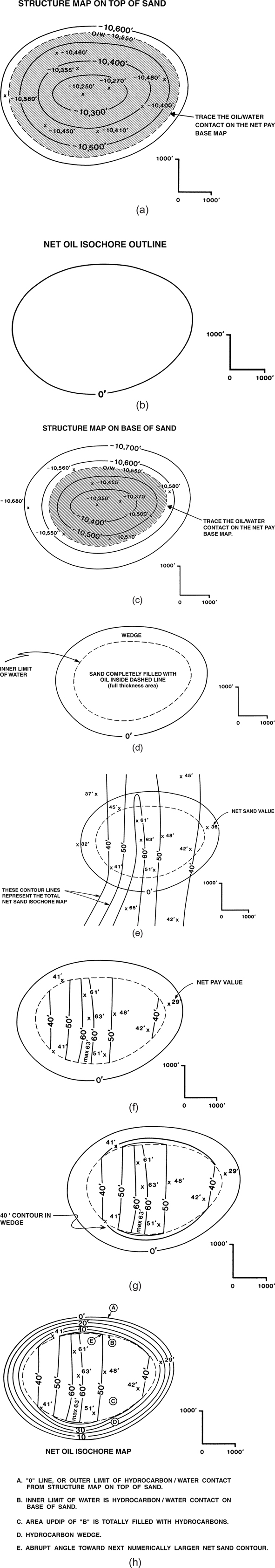
Figure 14-8 (a) Overlay a net oil basemap on the structure map of the top of sand (top of porosity). The oil/water contact is traced on the overlay. (b) The oil/water contact becomes the zero contour line on the net oil isochore map. (c) Overlay the net oil isochore map on the structure map of the base of sand (base of porosity), and trace the oil/water contact as a dashed line. (d) Isochore basemap delineating the two major areas comprising the net oil isochore map: (1) oil wedge from the zero line to the inner limit of water (ILW; oil/water contact on the base of the sand), and (2) the area of full hydrocarbon thickness. (e) To contour the full-thickness area, superimpose the net oil isochore map on a net sand isochore map and trace the net sand contours inside the ILW (dashed line). (f) Net oil isochore map with contours drawn for the oil-filled area. (g) All full-thickness area contours that intersect the ILW must connect through the wedge with contours of equal value (see text for procedure). (h) Completed net oil isochore map with important points of isochore construction listed. (From Tearpock and Harris 1987. Published by permission of Tenneco Oil Company.)
Start with a basemap with all the well control spotted.
Place the basemap over the structure map on the top of the unit (top of porosity) (Fig. 14-8a), and trace the outer limit of the productive reservoir. In this example, the limit is the oil/water contact on the top of the unit, and it becomes the zero line on the net oil isochore map, as in the previous example. The zero line is shown in Figure 14-8b. From this point forward, we refer to the base map as the net oil isochore map.
Place the net oil isochore map over the structure map on the base of the unit (base of porosity) (Fig. 14-8c), and trace the oil/water contact on the isochore map using a dashed line. This dashed line represents the inner limit of water (ILW) for the reservoir. Within the area inside this dashed line, oil fills the productive unit (Fig. 14-8d), and this area is referred to as the full-thickness area. The intersection of the oil/water contact with the top and base of the unit outline the wedge zone.
Post net pay values for all wells within the reservoir, corrected to true vertical thickness, on the net oil isochore map.
In the full-thickness area, the entire net sand is filled with oil, so the net oil in this area equals the amount of net sand, as interpreted on the net sand isochore map. Notice that the net sand contours are based on all wells within and outside the reservoir. Therefore, to contour the full-thickness area, place the net oil isochore map over the net sand isochore map as shown in Figure 14-8e, and trace the contours within the dashed-line area onto the net oil isochore map. Label the maximum thickness of oil (63 ft) within the area enclosed by the maximum net pay contour (60 ft). The full-thickness area of the net oil isochore map is now finished, as illustrated in Figure 14-8f.
The next step is to contour the oil wedge. The wedge zone is the area between the oil/water contact on the top of the unit and the oil/water contact on the base of the unit, as shown in Figure 14-8d and f. The oil wedge overlies a water wedge (see cross section in Fig. 14-10). All well data in the wedge must be honored. In the full-thickness area, net sand distribution controls the net pay contours. However, in the oil wedge, the structural attitude of the productive unit, and the distribution of impermeable rock within the unit influence the position of net pay contours. The contours conform in general to the structure contours, but they are not necessarily equally spaced (variations in contour spacing are discussed below). As the first step in contouring the wedge, draw the net pay contours from the full-thickness area into the wedge. Notice in Figure 14-8g that the full-thickness contour lines turn abruptly at the ILW, in the direction of increasing sand thickness (in the direction of the next net sand contour of higher value). They connect through the wedge with contours of the same value elsewhere in the full-thickness area. Lastly, draw the net pay contours in the oil wedge that do not correspond to contours within the full-thickness area. Honor the well data within the wedge, and more or less equally space contours where data is lacking (Fig. 14-8h). If the dip of the productive unit is more irregular than in this example, then that variation in structure may be considered in contouring the wedge.
The completed net oil isochore map is shown in Figure 14-8h. This figure highlights five important points of the net pay isochore map construction. We recommend that you leave the dashed ILW on the net pay isochore map. It allows others to review and verify that you have used the water contact on the base of porosity correctly in creating the net pay map.
The method of connecting the full-thickness contours to those in the wedge zone is extremely important and deserves special attention. Why can we not extend the net pay contours in the full-thickness area on trend, past the ILW and into the wedge? Look at Figure 14-9, which is similar to Figure 14-8g. Let’s discuss the construction of the easternmost 50-ft contour in the figure. Why must this contour line sharply change direction at the ILW on the net oil isochore map rather than continue straight into the wedge zone? Figure 14-10 is a diagrammatic cross section along the 50-ft net sand contour. The net sand is exactly 50 ft everywhere along the cross section. The net sand is exactly 50 ft everywhere along the cross section. In the portion of the reservoir that is up-dip to the oil/water contact on the base of porosity (ILW), oil fills the entire 50 ft of net sand. However, a point one foot down-dip of the ILW is within the wedge zone, where the sand contains both oil and water. Therefore, anywhere outside the ILW, both oil and water are present and, since the total net sand is still 50 ft thick, there must be less than 50 ft of oil. The 50-ft net pay contour, therefore, cannot continue along the 50-ft net sand contour down-dip of the ILW.
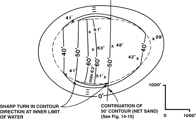
Figure 14-9 Full-thickness net pay contours make an abrupt turn at the inner limit of water toward the next net sand contour of higher value. (Modified from Tearpock and Harris 1987. Published by permission of Tenneco Oil Company.)

Figure 14-10 Cross section along the 50-ft net sand contour line in Figure 14-9.
Where must the 50-ft contour from the full-thickness area be drawn in the wedge zone? It must be drawn through an area of 50 ft of net oil in the wedge zone. This area exists only where the net sand is greater than 50 ft. In Figure 14-8e, notice that the net sand increases in thickness west of the 50-ft contour to a maximum of 63 ft. Therefore, the 50-ft contour, at its intersection with the ILW, must turn sharply toward the area of thicker sand. Since contour lines must close, the contour connects to the west to connect with the other 50-ft contour in the full-thickness area (Fig. 14-8g).
This procedure must be undertaken for all contour lines contained within the full-thickness area of the net pay isochore map. The correct application of this technique is most important. If the full-thickness area net pay contours are carried incorrectly into the wedge zone, the volume of hydrocarbons determined for the reservoir will be overestimated.
Figure 14-11a and b present a summary of the foregoing method for preparing a net pay isochore map for an edgewater reservoir containing one type of hydrocarbon.

Figure 14-11 (a)–(b) Summary of method for constructing a net hydrocarbon isochore map for an edgewater reservoir containing one hydrocarbon (oil or gas). (Modified from Tearpock and Harris 1987. Published by permission of Tenneco Oil Company.)
Comprehension of, and commitment to, the foregoing procedure will help you avoid the most common pitfall in net pay mapping, which is the mapping of more net pay than net sand that is filled with hydrocarbons. In the full-thickness area, a net pay contour corresponds exactly to a net sand contour. In the hydrocarbon wedge, a net pay contour corresponds to that same amount of net sand above the water level. Therefore, in the wedge, a net pay contour of a given value must be within an area where the total net sand is of greater value. Always overlay and compare the net pay contour map to the net sand contour map in order to check that the positions of the net pay contours are reasonable.
As with a bottomwater reservoir, you have two options if constructing a net pay isochore map of an edgewater reservoir on a computer workstation. First, you can follow the foregoing procedure on the workstation. The complication with this approach is that few if any software packages understand the implication of an ILW line when contouring net pay. In order to force the software package to duplicate the Wharton method, it may be necessary to add a significant number of digital control points to force the software to turn abruptly toward thicker net sand contours at the ILW.
A second option is to calculate the BRV of the reservoir on the computer and multiply this volume by a net/gross map to determine the net pay volume. This procedure is directly analogous to using the computer to construct a net pay map on a bottomwater reservoir except that a base of reservoir structure map is required in addition to a top of structure map and knowledge of the depth of the hydrocarbon/water contact. In this case, the base of reservoir structure map is combined with the surface representing the depth of the hydrocarbon/water contact. The volume between the top of structure and the combined base of structure/hydrocarbon/water contact is the BRV of the reservoir. Multiplying this volume by the net/gross map yields the net pay volume, which may then be contoured. As with a bottomwater reservoir, make sure to plot the net pay in each well within the accumulation to help in contouring the net pay volume. Make sure that all well control within the accumulation is honored because failure to honor well control is a red flag for anyone reviewing a net pay isochore map. It is still best practice to plot the ILW on the net pay isochore map. It is also best practice to construct a net sand map to compare with the net pay isochore contours in the full-thickness area and wedge zone.
Net Pay Isochore Map Construction for a Reservoir Containing Oil and Gas.
Two methods may be used to estimate the volumes of oil and gas in a reservoir containing both types of hydrocarbons. The simplest and quickest method is to construct a total net hydrocarbon isochore map and a net gas isochore map, calculate the volumes of each, and subtract the gas volume from the total hydrocarbon volume to determine the oil volume. This method is appropriate when only one lease owner is involved or when only the total estimated volumes of oil and gas are required (there being no interest in the actual distribution of oil and gas within the reservoir). Where a reservoir underlies two or more separate ownerships, it is very important to know the estimated volumes of gas and oil under each lease. In this case, net gas and net oil isochore maps must be constructed, preferably using the procedure outlined in this section.
Construct the net gas isochore map first. Draw the basic maps used in the Wharton method, which are the structure map on top of porosity, structure map on base of porosity, and net sand isochore map. Using these maps, construct the net gas isochore map as shown in Figure 14-12a and b. The net gas isochore map is constructed using the same procedure explained in the previous section on edgewater reservoirs containing one type of hydrocarbon. The only difference in this case is that the gas/oil contact defines the down-dip, outer limit of the gas reservoir, whereas in the previous cases the limit was determined by a hydrocarbon/water contact.
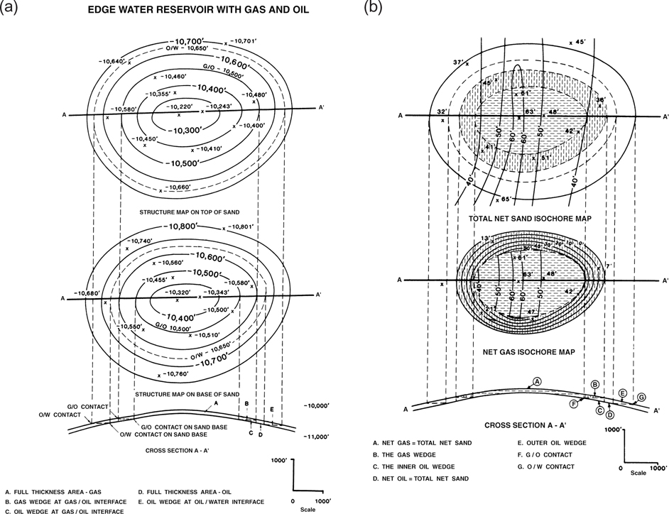
Figure 14-12 (a)–(b) Summary of procedure to construct a net gas isochore map for a reservoir containing both oil and gas. (Modified from Tearpock and Harris 1987. Published by permission of Tenneco Oil Company.)
The last map to be constructed is the net oil isochore map. This map differs from the previous maps in that it has two wedge zones, an inner wedge zone (gas/oil) and an outer wedge zone (oil/water), as shown on the cross section in Figure 14-12a. The outer oil wedge and any full-thickness areas are constructed using the Wharton method, as previously discussed; the inner oil wedge requires additional steps.
Figure 14-13a shows a partitioned map (without wells) for the oil reservoir, with an inner wedge and an outer wedge of oil, and an area of full-thickness in between. The fluid contacts on the structure maps are used to determine the zero net pay limits and dashed wedge limits by tracing them onto the net oil map.

Figure 14-13 (a) Outline of oil isochore map showing the inner and outer wedge zones and the full-thickness area. (b) Overlay of net oil isochore map on the net sand isochore map. The contours in the area of full oil thickness are equal to the net sand contours. (c) Full-thickness area is contoured. (d) Overlay of net gas and net sand isochore maps used to aid in the construction of the inner oil wedge contours. (e) Completed net oil isochore map. (From Tearpock and Harris 1987. Published by permission of Tenneco Oil Company.)
First, contour the area containing a full-thickness of oil. Post the net oil values next to each well and overlay the isochore basemap onto the net sand isochore map, as shown in Figure 14-13b. Trace the net sand contours on the net oil map only within the full-thickness area of oil, as shown in Figure 14-13c. Indicate the maximum thickness of oil in each of the areas enclosed by the 60-ft net pay contours. This portion of the isochore map is now complete.
As with edgewater reservoirs containing a single phase, edgewater reservoirs that consist of a gas cap and an oil rim can easily be isochored on a computer workstation. Using the procedures outlined previously for bottomwater and edgewater reservoirs, as appropriate, determine the bulk rock volume of the gas reservoir and the bulk rock volume of the oil reservoir. Multiply each volume by the net/gross map to determine the net pay volume for both the gas reservoir and the oil reservoir. Alternatively, you can determine the net pay volume of the gas reservoir and the net pay volume of the entire hydrocarbon reservoir and determine the net pay volume of the oil reservoir by difference.
We now contour the inner oil wedge on the map, to be followed by contouring of the outer oil wedge. By referring to the cross section in Figure 14-12b, we see that within the inner oil wedge, the sum of net oil-filled and net gas-filled sand equals the total net sand. Therefore, in order to determine the amount of net oil in the inner wedge zone, the following procedure is used. Overlay the net gas isochore map on the net sand isochore map, and note each location where the contours on the two separate maps cross. The net oil sand value at each contour intersection is equal to the difference in values of the two contours. For example, at point C in Figure 14-13d, the 30-ft contour line on the net gas isochore map crosses the 50-ft contour line on the net sand isochore map. By subtracting the 30 ft of net gas from the 50 ft of net sand, a value of 20 ft of net oil is obtained for this point. Take a minute and review the data at point D. As indicated, a known value is established wherever a contour line on the net gas isochore crosses a contour line on the net sand isochore. The net oil sand value at each intersection is the difference in values of the two contours. Figure 14-13d shows 48 points of control, plus data from four wells, to aid in contouring the inner wedge zone of the oil isochore map. Overlay the net oil map on the net gas and net sand maps, mark selected points with the corresponding value of oil, and then contour the inner oil wedge. The net pay contours at the edge of the full-thickness area turn abruptly towards the thicker net sand values (Fig. 14-13e), just as described in the contouring of a single-phase reservoir.
When contouring the inner oil wedge, the net oil isochore map should be overlain on both the net gas and net sand isochore maps. This allows mapping the inner oil wedge with the constraint, and thus the assurance, that the sum of the net gas and net oil does not exceed the total net sand. This is one of the most complex, and therefore most difficult, areas to construct within an isochore map.
Finally, contour the outer wedge precisely as described in the previous section on contouring the wedge in a single-phase reservoir (Fig. 14-8h). We now have constructed the inner and outer wedges and the full-thickness area for the oil isochore. The completed net oil isochore map is shown in Figure 14-13e.
Methods of Contouring the Hydrocarbon Wedge
Limited Well Control and Evenly Distributed Impermeable Rock
With limited well control in the wedge zone of a reservoir and a fairly even distribution of impermeable rock within the productive unit, the most common method for contouring the wedge is to combine proportional and equal spacing of the net pay contours, while honoring the available well control. This is how the outer oil wedge and gas wedge in the last example were constructed. Typically, you may equally space contours between the outermost wells and the zero net pay contour. Within the area of well control, proportionally space the contours according to the net pay values and the well locations. Contouring in this manner assumes that the vertical distribution of net sand is uniform in the reservoir. On the other hand, the horizontal distribution of net sand may not be uniform and, if so, the net pay contours will reflect that stratigraphy only to the extent of the density of control points. The configuration of the contours within a wedge is primarily controlled by the structural attitude of the productive unit and the distribution of net sand and impermeable rock within the overall unit. If the distribution of nonreservoir-quality rock (e.g., shale) is fairly uniform both vertically and horizontally, the primary influence on the contours in the wedge is the structural attitude of the unit. In such a case, the contours should more or less conform to the structure contours and be more or less proportionally and equally spaced.
If the well control in the wedge is limited and sand distribution varies significantly horizontally, we can use the ratio of net sand to gross interval (net/gross ratio) within the productive unit to approximate net pay within the wedge. This allows us to more accurately contour in the wedge than if we simply equally and proportionally space the contours. Using the wells within and outside the reservoir, first calculate the net/gross ratio in each of the wells. Then map the net/gross ratio in the area of the reservoir, using contours with a typical contour interval of 5% or 10% (0.05 or 0.10). When we map the net/gross ratio, we make the assumption that the distribution of net sand is uniform vertically. This means that, at any point in the reservoir, the net/gross ratio is the same above the water level as it is for the entire thickness. Once the map is complete, estimate the net pay at selected points in the wedge. At a given point, calculate the gross interval thickness above the water level as the difference in depth between the top of porosity and the water level. Multiply this calculated gross interval by the net/gross ratio to estimate the net sand above the water level, which is equal to net pay at the selected point.
This process is done automatically if you use the workstation to compute the BRV of the reservoir and multiply it by a net/gross map. Lateral changes in gross thicknesses are captured by the bulk rock volume. Lateral changes in the net/gross ratio are captured in the net/gross map.
We use the maps in Figure 14-14 as an example of the technique, applied to an edgewater gas reservoir with a gas/water contact at −8350 ft. The net/gross mapping technique begins after construction of the outline of the net pay map and contouring of net pay within the full-thickness area (Fig. 14-14b). As the first step in constructing a net/gross ratio map, calculate the net/gross ratio for wells within and outside the reservoir. Figure 14-14a shows the net/gross ratio calculation beside each well in the area of study. Contour the values using a contour interval of 5%, or 0.05. Then estimate net pay at selected points within the wedge. Figure 14-14b is a partially completed net pay isochore map of the reservoir, shown as an overlay on some contours in the net/gross map. For efficiency, select estimated net pay points to lie directly on the net/gross contours, such as points (1) through (9). As an example, use point (3) on the 50% contour. Calculate the gross interval thickness above the water level at point (3) by taking the difference in depth between the gas/water contact at −8350 ft and the top of porosity at point (3), which is −8310 ft on the structure map (not shown). The gross interval thus equals 40 ft. Then estimate the net pay by using the following calculation.
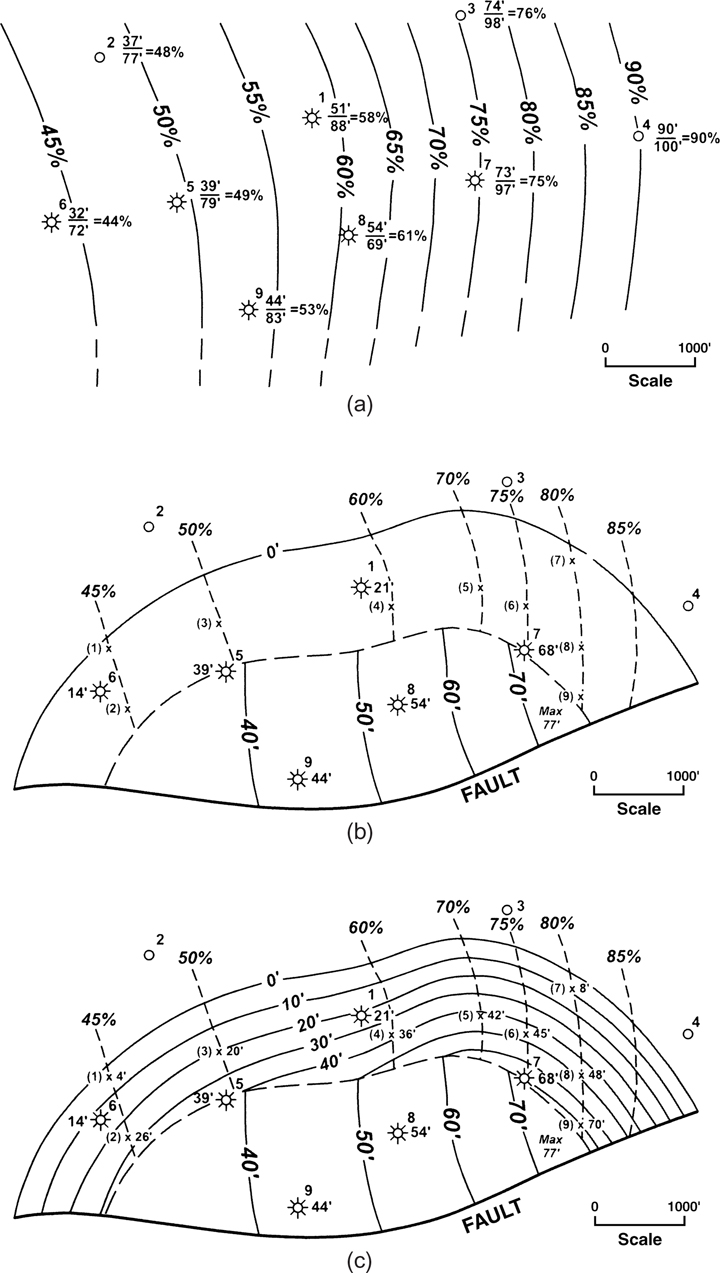
Figure 14-14 (a) Net/gross ratio map based on well control. (b) Overlay of partially completed net gas map on the net/gross ratio map. (c) Completed net gas isochore map. (Published by permission of D. Tearpock.)
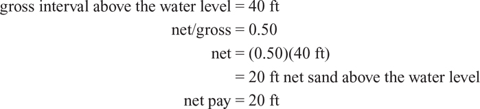
Using the same procedure, create as many points of estimated pay as necessary for adequate control. Figure 14-14c shows the completed net pay map for the reservoir. If using the BRV multiplied by net/gross map method to calculate net pay using a workstation, this process will be utilized automatically.
The net/gross mapping method provides added control for contouring net pay in the hydrocarbon wedge. The method is reasonably accurate if net sand is more or less uniform in vertical distribution. However, the method is significantly less accurate if the reservoir includes intervals of impermeable rock that vary considerably in thickness. For a reservoir with this erratic vertical distribution of net sand and impervious rock, we recommend estimating net pay by using the walking wells method, described in the next section.
Walking Wells—Unevenly Distributed Impermeable Rock
A technique called walking wells can be used to improve the accuracy of the contouring in the hydrocarbon wedge. At times, we may wish to better define the distribution of net pay sand within the wedge instead of just using the proportionally spaced method. For example, a dispute exists as to the equity of various leases overlying a reservoir, and the reservoir is being mapped for equity determination between various companies. Furthermore, the distribution of net sand versus impermeable rock varies within the reservoir, such as both thick and thin shale intervals occurring within the productive unit. In such cases, a more detailed estimate of the reserves in the wedge zone may be required.
Our purpose in walking a well is to estimate the net pay at selected points within the wedge. To accomplish this, we assume that the stratigraphy seen in a given well log is representative of the stratigraphy along a designated net sand contour line extending through the wedge. In our imagination, we will move, or walk, the well along this line and estimate net pay at selected points, as described below.
Let’s say we wish to construct a net gas isochore map, with a 10-ft contour interval, for a sandstone reservoir with limited well control. We want additional control in the gas wedge, so we decide to walk a well through the wedge and estimate the amount of net gas at selected points. Any well to be walked can be located in the reservoir itself, or even down-dip of the hydrocarbon/water contact and thus outside the reservoir. The key point in walking a well is to choose a well that can be walked parallel to the nearest contour line on the net sand isochore map. This is a critical point because when walking a well through the wedge, the assumption is made that the amount and distribution of net sand, as seen in the well log, are the same within the reservoir in a direction parallel to the net sand contours. For example, if a well has 50 ft of net sand, it will fall on the 50-ft total net sand contour line. Construction of this 50-ft contour line assumes that exactly 50 ft of net sand exists all along this contour line, not just at the well location (Fig. 14-15). If a series of wells were drilled along this contour line, each well should encounter exactly 50 ft of net sand. We further make the assumption that along the net sand contour line (at least for any limited distance), the vertical distribution of net sand and impermeable rock, as seen in the well, remains constant within the unit being mapped. This assumption regarding the rock distribution may not be true along the 50-ft contour over long distances, or on opposite limbs of a fold, because of changes in depositional environments, variable structural growth histories, and other factors. However, it is a reasonable assumption to make for a limited distance from the well, parallel to the nearest net sand contour line.
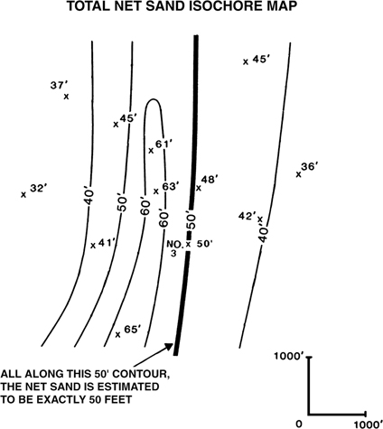
Figure 14-15 Net sand contour map. Each net sand contour line is constructed with the assumption that the amount of net sand is constant along the contour line.
Procedure for Walking a Well.
Use three maps in walking a well through the wedge zone. First, lay the structure map of the top of porosity over the net sand isochore map. Then overlay the net gas base map on the two maps, as shown in Figure 14-16a. We wish to walk Well No. 2, which is located near the crest of the structure, through the wedge zone in order to estimate net pay in part of the reservoir. We walk the well along the dashed line, parallel to the 50-ft net sand contour.
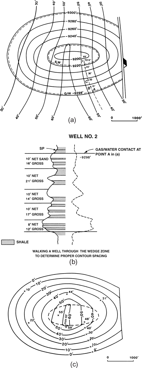
Figure 14-16 (a) Net gas basemap overlain on top-of-porosity structure map and net sand isochore map. Walk Well No. 2 through the wedge zone along the dashed line, parallel to the nearest net sand contour line (50 ft). (b) Five-inch detailed log for the 9200-ft reservoir, showing increments of 10 ft of net sand per gross feet of interval. (c) Completed gas isochore map for the 9200-ft reservoir. The contour spacing in the southeastern portion of the wedge zone was improved by walking Well No. 2. (From Tearpock and Harris 1987. Published by permission of Tenneco Oil Company.)
Notice that the ILW is shown on the structure map of the top of porosity as a means to delimit the full-thickness area on this map. From its position on the base-of-porosity structure map, the ILW was simply traced on the top-of-porosity structure map. Now we have the data necessary to make a net pay isochore map after walking the well, as described in the following procedure.
Preparatory to walking a well, use a computer analysis of the digital log curves or an analysis of a detailed 5-in. electric log to determine the net sand in the well and the distribution of sand and impermeable rock. The 5-in detailed electric log for Well No. 2 is shown in Figure 14-l6b. The well contains 48 ft of net sand, and the log shows increments of 10 ft of net sand per gross feet of interval, so chosen because we use a 10-ft contour interval in the net pay map. The productive unit is full of gas in Well No. 2, at its position in the full-thickness area.
Overlay the top-of-porosity structure map on the net sand map, then overlay the net gas basemap. Trace the gas/water contact as a zero net gas contour on the basemap, and trace the limit of the full-thickness area as a dashed line.
On the net gas map, lightly mark a dashed line for the well path, parallel to the nearest net sand contour. The net sand contour map may be removed for now; use it later in net pay mapping of the full-thickness area and for checking positions of net pay contours in the wedge.
To begin walking Well No. 2, move the well, from its actual structural position, along the well path and place it such that the top of porosity in the productive unit is at the gas/water contact at −9298 ft, which corresponds to the zero contour line on the net gas isochore map (Point A in Fig. 14-16a). A well drilled at this location would (1) encounter the top of porosity of the productive unit at the gas/water contact, (2) contain 48 ft of net sand, and (3) have no pay.
Starting at the top of the sand on the electric log, determine the number of vertical gross feet of section containing 10 ft of net sand. In Figure 14-16b, a total of 16 ft of gross section includes the 10 ft of net sand. From Point A, move the well up-structure 16 ft, along the dashed line to locate Point B at −9282 ft. This Point B becomes a 10-ft net gas data point for contouring the gas wedge, because a well drilled at Point B would encounter the top of the sand 16 ft above the gas/water contact, and it would contain 10 ft of net gas sand.
To determine the location of the 20-ft net gas point, start at the base of the previous 10-ft net sand section in the log and repeat the procedure. In this example (Fig. 14-16b), it requires 21 vertical gross ft to obtain the next 10 ft of reservoir-quality sand. Move the well up-structure 21 ft from Point B, along the dashed line, to locate Point C at −9261 ft. Point C is the 20-ft net gas data point at 37 ft (16 ft + 21 ft) above the water level.
Continue the same procedure until the well is back at its original structural position. Erase the dashed well path on the net gas map.
Using this method, the well may be walked completely across the wedge, resulting in a more accurate contour spacing than using the method incorporating equal spaced and proportionally spaced contours. We make no assumption about the vertical distribution of net sand being uniform. We use the real distribution of net sand in an actual well to estimate net sand distribution in a part of the reservoir. Figure 14-16c shows the completed net gas isochore map constructed for this reservoir, incorporating the data obtained from walking Well No. 2.
We can walk as many wells as we deem necessary. However, we emphasize strongly that a well must be walked parallel to the nearest contour line on the net sand isochore map. Significant net pay contouring errors can occur if this procedure is not followed. Consider Well No. 5 in the western portion of the reservoir (Fig. 14-17). If we wish to develop a more accurate contour spacing in this area of the reservoir, can Well No. 5 be walked from the water level up-dip to the inner limit of water, along the dashed line? The answer is no. Well No. 5 has 28 ft of net sand. If the well is walked from the gas/water contact up-dip, it will be walked across net sand contours into an area of greater net sand than is actually present in the well, as seen on the net sand map. Therefore, Well No. 5 cannot be walked to improve the contour spacing in this area of the wedge. Caution must be taken when walking wells to be sure that the assumptions made in choosing a well to walk are geologically reasonable and can be supported by a net sand isochore map or, if necessary, additional study of sand distribution.
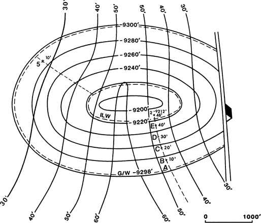
Figure 14-17 Structure map superimposed onto the net sand isochore map. Well No. 5 in the western portion of the reservoir cannot be walked through the wedge zone to improve the spacing of net pay contours. (Modified from Tearpock and Harris 1987. Published by permission of Tenneco Oil Company.)
Reservoirs with Significant Shale Intervals.
If a reservoir is encountered with one or more significant shale intervals between net sand, such as that shown in Well No. 2 in Figure 14-18a, the accurate construction of the net hydrocarbon isochore map within the wedge may depend on the walking of wells through the wedge. It is obvious from a review of the 5-in. detail log for Well No. 2 that the net sand and impervious rock are not evenly distributed throughout the gross interval. Therefore, the use of the equally spaced contour method for contouring the wedge would result in significant error.

Figure 14-18 (a) Five-inch detailed electric log for Well No. 2. The sand and impermeable rock are not evenly distributed throughout this productive unit. (b) Top-of-porosity structure map superimposed on the net sand isochore map. The dashed lines indicate paths along which Wells No. 2 and 3 were walked through the wedge zone to improve the net gas contour spacing. (From Tearpock and Harris 1987. Published by permission of Tenneco Oil Company.)
The map in Figure 14-18b shows the location of Well No. 2, in its position on structure, and the placement of the 10-ft and 20-ft net gas values used for contouring the net gas isochore map based on walking Well No. 2 through the wedge. Notice that the first 10 ft of net sand are obtained in 16 ft of gross interval; however, it takes another 52 ft of gross interval to obtain another 10 ft of net pay sand. Therefore, the estimated 10-ft net gas point is at −9282 ft (16 ft above the water level of −9298 ft), and the estimated 20-ft net gas point is at −9230 ft (68 ft above the water level). Well No. 3 was also walked to generate the 10-ft and 20-ft net gas points shown in Figure 14-18b.
Figure 14-19a shows a net gas isochore map prepared for this reservoir using a combination of equally spaced and proportionally spaced contours within the wedge, which honor the net pay values assigned to each well. Figure 14-19b is a net gas isochore map prepared by walking Wells No. 2 and 3 through the wedge. Observe the significant difference between the two net gas isochore maps. If there were several leases involved in this gas reservoir, the net gas isochore map prepared by walking the wells would provide a more accurate map for assigning equities to each lease.

Figure 14-19 (a) Net gas isochore map based on equally and proportionally spaced contours. (b) Net gas isochore map with the contour spacing based on walking Wells No. 2 and 3 through the wedge. Compare this map to that shown in Figure 14-19a. (From Tearpock and Harris 1987. Published by permission of Tenneco Oil Company.)
Several other methods exist for constructing accurate net pay isochore maps. For example, there is a more accurate method of estimating pay when we walk wells. Also, using the method that employs the construction of a net-to-gross ratio map for the entire productive unit provides estimates of net pay at points within the wedge. In this section of the chapter, we review the more detailed method of walking wells.
Using the same reservoir as in Figure 14-18, we illustrate the more detailed technique of walking wells. Figure 14-20 shows a north-south diagrammatic cross section along the path used to walk Well No. 2. On the right side of the figure, we position Well No. 2 so that the top of the sand is at the gas/water contact (−9298 ft). On the left side of the figure, we position the well at the inner limit of water (−9218 ft) where the base of porosity is at the gas/water contact. From the right, Well No. 2 must be walked 16 ft up-structure from the gas/water contact to −9282 ft, to obtain 10 ft of net pay sand. From this point up-dip to −9248 ft, the well gains no additional pay because the section being raised above the water level contains nothing but shale. At −9248 ft, the net pay remains 10 ft. At this point, the gas/water contact intersects the top of the lower sand member; therefore, moving up-structure from this position, the well gains additional pay. Continuing to walk the well up-dip, it must reach −9230 ft before an additional 10 ft of net sand, in the lower member, lies above the water contact. We estimate 20 ft of net pay at −9230 ft. At the edge of the full-thickness area, with the gas/water contact on the base of sand, all the net sand (28 ft) lies above the water contact. From this point to the actual well location, shown on the far left in the figure, the reservoir contains 28 ft of estimated pay.
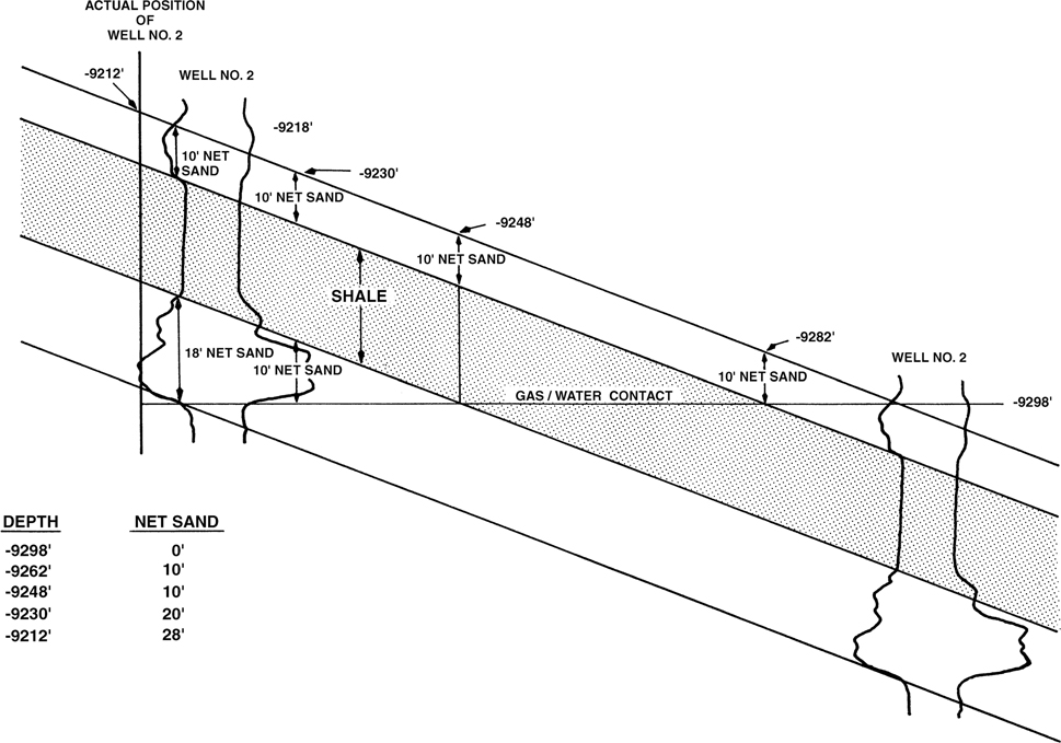
Figure 14-20 Diagrammatic cross section along the path taken to walk Well No. 2.
On the cross section, two locations have 10 ft of net gas sand (−9282 ft and −9248 ft), and the area between these points has a constant 10 ft of net gas sand. The accuracy of the net gas isochore map can be improved by constructing a map honoring the two 10-ft net pay values. Well No. 3 was also walked through the wedge zone, as indicated in Figure 14-18b, to aid in the construction of the net pay isochore map.
Figure 14-21 shows the resulting net gas isochore map. At first glance, it may appear as if an important contouring rule was broken in the construction of the isochore map: contours cannot merge or split. However, no rules are broken. The two 10-ft contour lines that appear to merge represent the limits of a very wide 10-ft contour line. Everywhere within the area of the wide contour, the net gas has a constant value of 10 ft.
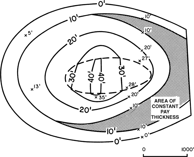
Figure 14-21 Net gas isochore map using a more accurate method of contouring the wedge based on the results of walking Wells No. 2 and 3.
One may ask, since the sands are so far apart and separated by such a thick shale break, why we would not map each sand separately and construct two isochore maps. In the western part of the reservoir, some of the sands within the two sand members shale-out, and sands develop within the thick shale interval. The result is a reservoir consisting of interfingering shales and sands in which there is productive communication throughout the reservoir, with the sands acting as a single reservoir. Therefore, the thick shale wedge is localized in the eastern section of the reservoir. The rapid decrease in width of the 10-ft contour line reflects the fact that the shale interval decreases to the west. If such a shale interval were known to be continuous over the entire reservoir, it would be necessary to prepare a structure map for each sand member and construct a separate net pay isochore map for each sand member.
The procedure outlined in this section is more involved than the two previous methods shown, but the technique provides further accuracy in the construction of a net hydrocarbon isochore map. The method chosen to prepare a net hydrocarbon isochore map depends on a number of factors, including the available time, detail, and accuracy required.
Vertical Thickness Determinations
True vertical thickness (TVT) is the thickness of an interval measured in a vertical direction. As mentioned in several sections of the text (see Chapter 4), vertical thickness is a very important measurement. It is this vertical thickness that is required to measure the vertical separation (equal to missing or repeated section in a well) of a fault. It is also the thickness required to accurately count net sand and net pay from 5-in. detailed logs, and it is the thickness used to construct net sand and net pay isochore maps. As described in the introduction to this chapter, the vertical thicknesses of net sand and net pay typically represent aggregate vertical thicknesses.
In a vertical well, the actual thickness measured on the electric log is the TVT. In the case of a directionally drilled well, however, a correction factor must be applied to correct the exaggerated or diminished measured log thickness (MLT) to TVT.
For a horizontal reservoir (zero bed dip), the thickness that is used for net sand or net pay isochore mapping equals the true stratigraphic thickness (TST) (Fig. 14-22). However, if the same reservoir is rotated to some angle, such as 20 deg, the thickness of the reservoir required for net sand and net pay isochore mapping does not equal the stratigraphic thickness. Figure 14-22 illustrates the cross-sectional area of a reservoir with a fixed width in the third dimension, and we use the cross section to represent the volume of the reservoir. The horizontal reservoir (zero bed dip) in the lower portion of the figure has a cross-sectional area of 50,000 sq ft. The reservoir has a length of 500 ft, as seen in map view, and a thickness of 100 ft. Since the dip of the reservoir is zero, the TVT equals the TST (100 ft). If the same reservoir rotates to an angle of 45 deg, as shown in the upper portion of the figure, the length of the reservoir shortens to 354 ft in map view. The cross-sectional area of the reservoir does not change, as the TST remains 100 ft. In order to map the reservoir and maintain a cross-sectional area of 50,000 sq ft, the thickness to be used must exceed 100 ft. The TVT of the dipping reservoir measures to be 141.25 ft, and 141.25 ft × 354 ft = 50,002.5 sq ft. We conclude from this example that as a reservoir of fixed length rotates from the horizontal, the areal extent of the reservoir decreases in map view; therefore, in order to maintain the same cross-sectional area or volume of the reservoir, the shortened length must be multiplied by the TVT.
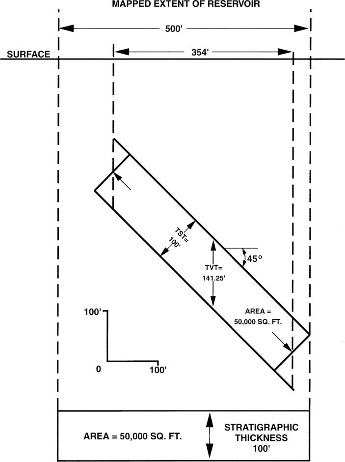
Figure 14-22 Cross-sectional area of two reservoirs of equal volume and a constant TST of 100 ft. One reservoir is horizontal, the other is dipping at 45 deg.
For directionally drilled wells, the log thickness of a given stratigraphic interval can either be thicker, equal to, or thinner than that seen in a vertical well drilled through the same stratigraphic section. A correction factor must be applied to the MLT in most deviated wells to convert the borehole thickness to TVT. The correction factor consists of two parts: (1) the correction for wellbore deviation angle within the interval of interest, and (2) the correction for bed dip. Any one of Eqs. (4-3), (4-4), (4-5), or (4-6) in Chapter 4 may be used to calculate this correction factor. In Chapter 4, we used the equations to estimate the TVT of missing or repeated section in a well as the result of a fault. Remember, the vertical separation of a fault at a well equals the TVT of the stratigraphic section missing or repeated in the wellbore. In this chapter, we look at the same correction factor equations in order to convert deviated wellbore thickness to TVT, for use in net sand and net pay isochore mapping.
For convenience, we repeat the correction factor given in Eq. (4-6), presented here as Eq. (14-1). Equation (14-1), which is a 3D equation, is the preferred equation to use for correction factors because this one equation can be used to calculate the thickness correction factor regardless of the direction of wellbore deviation, and the true dip of the beds is used instead of the apparent dip required in the 2D equations. Recall from Chapter 4 that we refer to this equation as Setchell’s equation:
where
If the beds are horizontal, then Setchell’s equation reduces to the simple correction factor equation given in Chapter 4, Eq. (4-3):
which is equivalent to correcting for wellbore deviation only.
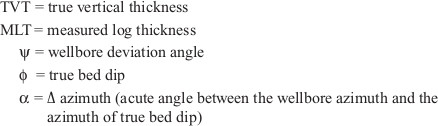
Figure 14-23 illustrates the measurement of azimuth and ∆ azimuth for use in Eq. (14-1). For convenience, the ∆ azimuth used in the equation is typically the acute angle between the azimuth of the wellbore and the azimuth of the true bed dip.
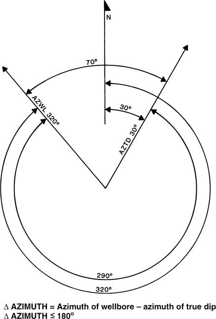
Figure 14-23 Azimuth is measured from 0 deg to 360 deg in a clockwise direction from true north. A ∆ azimuth is the difference in azimuth of the wellbore and the azimuth of true bed dip. For convenience, the minimum ∆ azimuth is typically used.
In order to more closely examine the two directionally drilled wells shown in Figure 14-24, look first at the well drilled to the east in a down-dip direction (Fig. 14-24a). Consider the interval to be a reservoir filled with gas or oil. The reservoir has an MLT of 476 ft. We apply the correction factor for wellbore deviation only, using Eq. (4-3) from Chapter 4. The MLT reduces to 357 ft, shown in the figure as the TVD thickness, or the true vertical depth thickness (TVDT). This thickness also exceeds the TVT of the interval, because the correction for only wellbore deviation does not take into account the dip of the beds. The TVDT is that thickness of an interval obtained from a true vertical depth (TVD) log and, for dipping beds, TVDT does not equal TVT (see Chapter 4). With the final correction for bed dip, the MLT converts to the TVT of 150 ft, shown in Figure 14-24a at the penetration point of the wellbore in the top of the reservoir. Note that the TST is 123 ft. The TST is calculated by multiplying the TVT by the cosine of the angle of bed dip (35 deg in this example).
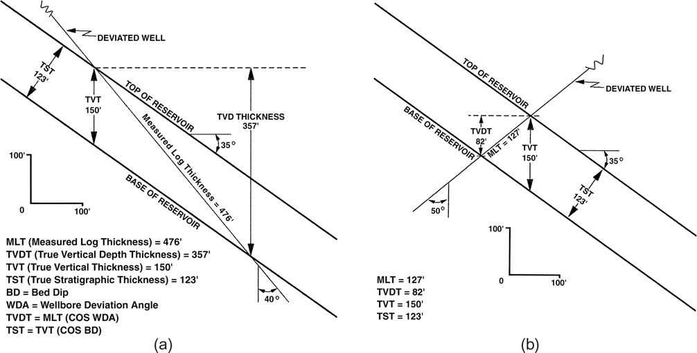
Figure 14-24 (a) TVT correction for a well drilled in a down-dip direction. (b) TVT correction for a well drilled in an up-dip direction.
The well in Figure 14-24b deviates up-dip, to the west. The MLT of 127 ft measures less than the TVT. Applying a correction factor for the well deviation angle alone, which is equivalent to the correction to TVDT, provides an even smaller thickness of 82 ft. When Eq. (14-1), the correction factor equation for both bed dip and wellbore deviation, is applied, the MLT converts to the TVT of 150 ft, the value needed for net sand and net pay mapping. As an exercise, use Eq. (14-1) to calculate the TVT for the two wells in Figure 14-24 and to confirm the results shown.
Various computer programs can be used to create TVD, TVT, and TST logs from measured depth (MD) logs for use in mapping. The deviated well log data, the directional survey for the well, and bed dip information are necessary as input data. The log data are obtained from the logging company tapes or digitized from the actual log. The directional survey data are furnished by the directional company that worked the well. The bed dip information can be obtained either from completed structure maps or from a dipmeter. The output logs can be in standard presentation or at any scale desired. The logs in Figure 14-25 were created by using IEPS (Integrated Exploration and Production System). The log sections for Well No. MP-D5, shown from left to right in the figure, represent the (1) measured depth log, (2) true vertical depth log, (3) true vertical thickness log, and (4) true stratigraphic thickness log. This well is in an area of significant bed dip. Notice the similarity of the MD log and the TVD log. This is so because the TVD log thickness is equivalent to a correction for wellbore deviation only, and not bed dip. However, the TVT log shows a considerable reduction in thickness from the MD log because the TVT log reflects corrections for both wellbore deviation and bed dip.
Figure 14-25 Computer-generated electric logs illustrating the difference in thickness between measured depth, true vertical depth, true vertical thickness, and true stratigraphic thickness logs, generated for the same well. (From Tearpock and Harris 1987. Published by permission of Tenneco Oil Company.)
We caution here that TVD logs, which are a standard part of the log suite for a deviated well, are used too often for purposes that are not applicable with this log. A widespread misunderstanding exists that a TVD log prepared from a MD log can be used to (1) correlate with other well logs, (2) determine the vertical separation for a fault, and (3) count net sand and net pay for isochore mapping. Remember, a TVD log is corrected only for wellbore deviation, and not bed dip. In areas of flat-lying beds, a TVD log is equivalent to a TVT log because the only correction factor required is for wellbore deviation (Fig. 14-26). However, if the beds are dipping (particularly over 10 deg), a TVD log typically does not represent the log thickness required to aid in correlation work, to determine the vertical separation for a fault, or for use in net sand and net pay counting. For these purposes, we must correct a deviated well log so that the log thickness represents the TVT. Look again at Figure 14-25 and observe the significant difference in thickness between the TVD and the TVT logs. To determine the vertical separation of a fault by correlation of a faulted well with a deviated well, and to count all net sand and net pay from a deviated well log, we must use a TVT log or its equivalent. By the equivalent of a TVT log, we mean calculating and using correction factors if a TVT log is unavailable, which is commonly the case. Therefore, for each interval on the deviated well log requiring the conversion of MLT to TVT, determine correction factors and apply them to the MLTs of the intervals of interest.
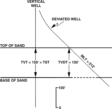
Figure 14-26 True vertical depth thickness equals true vertical thickness where the stratigraphic unit is horizontal.
The Impact of Correction Factors
Figure 14-27 presents an example of two separate net pay isochore maps prepared for a reservoir on the flank of a salt dome in the offshore Gulf of Mexico. Notice that there are two platforms from which wells were drilled. Platform D is located in the up-structure position, with the D Platform wells directionally drilled down-dip. The A platform is located on the flank of the structure, with most of the A Platform wells directionally drilled up-dip.
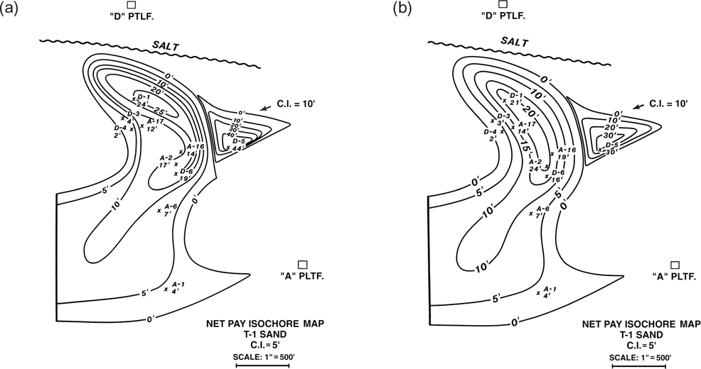
Figure 14-27 (a) Net pay isochore map for the T-1 Sand, Reservoir A. The net pay values for the deviated wells from Platforms A and D were corrected only for wellbore deviation. (b) Net pay isochore map for the T-1 Sand, Reservoir A. The net pay values for the deviated wells from Platform A and D were corrected for wellbore deviation and bed dip. Compare the net pay value for each well with those shown in Figure 14-27a. (From Tearpock and Harris 1987. Published by permission of Tenneco Oil Company.)
Figure 14-27a shows a net pay isochore map prepared for the T-1 Sand, Reservoir A. The net pay values posted on the net pay isochore map were corrected for borehole deviation, but not for bed dip of about 35 deg at this location on the flank of the structure. In addition to the error of failing to correct the net pay values for bed dip, several other serious isochoring problems exist but are not discussed here.
Figure 14-27b presents a net pay isochore map for the same reservoir with new net pay values, which were generated after correction for borehole deviation and bed dip. This new isochore map was prepared solely to compare the effect of the correction factor for bed dip on the ultimate calculation of the total volume of the reservoir. Therefore, the isochore errors made in Figure 14-27a (not discussed here) are incorporated in the net pay isochore map in Figure 14-27b. The planimetered volume for the isochore map in Figure 14-27a, with MLTs corrected for bed dip, is 524 acre-feet, whereas the map in Figure 14-27b with uncorrected MLTs provides a volume of 617 acre-feet. Therefore, the estimated hydrocarbon volume for the map prepared without correcting the net pay thickness values for bed dip is 18% greater than the isochore map prepared by taking into account the correction factor for bed dip. So, based on the incorrect map, the volumetric calculation overstates the reserves by 18%.
In a situation like this, we would expect the error factor to be larger than 18%, and it would be in most cases. However, look at Wells No. A-2 and D-5. Well No. A-2 was corrected upward from 17 ft net pay to 24 ft net pay, whereas Well No. D-5 was corrected downward from 44 ft net pay to 30 ft net pay. It so happens that the D Platform wells, drilled down-dip, result in a reduction in net pay values when the correction factor for bed dip is considered, whereas the A Platform wells, drilled up-dip, result in an increase in net pay. Therefore, a significant part of the error is negated because of the directions in which the wells were drilled.
This reservoir is only one of a number of oil and gas reservoirs that are productive within this field. A complete remapping of the field was undertaken when several major mapping errors, such as the one shown here, were identified. The remapping of the field resulted in a significant write-down of hydrocarbon reserves that were overestimated because of mapping errors, such as the failure to incorporate the proper correction factors in determining net pay values. Several development wells planned for the field based on the overestimated reserves were not required, saving the company millions of dollars in unnecessary wells. This example illustrates the impact that correction factors can have on estimated hydrocarbon volumes determined from volumetric calculations using net pay isochore maps.
We have seen error factors of several hundred percent. In one example, the net pay used for the reserve estimate from a deviated well was 750 ft, when in fact the actual TVT value was about 150 ft. This is a major error, resulting in a significant overestimation of reserves.
TVT Correction (Setchell’s Equation) Discussion
If one closely examines Figure 4-22, the TVT value that is being calculated is the TVT at the point where the well exits the bed and the bed dip that is used in this derivation is the dip of the top of the bed. The top and the base of the bed are parallel in Figure 4-22, so the TVT at the point where the well exits the bed is equal to the TVT where the well enters the bed. Indeed, the TVT is constant along the entire length of the well within the bed if the bed boundaries are parallel. If the bed boundaries are parallel, the TVT value of the bed can be posted at both the point where the well enters the bed and the point where it exits the bed or anywhere along the path of the well within the bed. If the values at both points and along the well path do not fit the isochore map, it indicates that the top and base of the bed are not parallel. Consider, for example, a hypothetical deviated well drilled from west to east near the crest of the structure in Figure 14-14c. If this well penetrated the top of the reservoir just west of Well No. 9, the gross interval thickness would be expected to be about 80 ft, based on the 83 ft of gross interval thickness seen in Well No. 9 (Fig. 14-14a). If the well penetrated the base of the reservoir near the 70-ft net gas contour line, the gross thickness would be expected to be about 100 ft (70 ft of net sand divided by NTG of about 0.73). Obviously, in the case of this reservoir, the top and base of the reservoir are not parallel.
Although the derivation of the Setchell equation shown in Figure 4-22 uses the dip of the top of the bed and calculates the TVT of the bed at the point where the well exits the bed, we could equally easily derive the equation for the TVT where the well enters the top of the bed using the dip of the base of the bed. The fact that the TVT at the point of exit of the bed uses the dip of the top of the bed and the TVT at the point of entry into the bed uses the dip of the base of the bed makes intuitive sense. We know the depth of the base of the bed at the point of exit. To determine the TVT of the bed at this point, we need to know the depth of the top of the bed at the point of entry and the dip of the bed to a point directly above the exit point. The dip of the base of the bed is irrelevant to this determination. An analogous argument can be made for determining the TVT at the point of entry to the bed.
If the top and base of the bed being isochored are not parallel, the Setchell equation, Eq. (14-1), can be used to determine the TVT at both the point of entry into the bed and the point of exit out of the bed.
Consider the well illustrated in Figure 14-24a, which is drilled directly down-dip at an inclination of 40 deg through a bed with the top of the bed dipping at 35 deg. We have shown that if the well has an MLT of 476 ft, the TVT where the well exits the bed is 150 ft. Consider if the base of the bed is not parallel to the top of the bed but dips at 40 deg rather than 35 deg. In this case, we can use Eq. (14-1b) to determine that the TVT of the bed is 108 ft at the point the well enters the bed [476 × (cos 40 − (sin 40 cos 0 tan 40) = 108]. This result makes intuitive sense. If the base of the bed dips more than the top of the bed, the bed must be expanding down-dip. If we know that the TVT of the bed is 150 ft where the well exits the bed, the TVT up-dip where the well enters the bed must be less than 150 ft.
If the azimuth of the dip of the top of the bed differs from the azimuth of the base of the bed, α will have to be adjusted in the two equations.
Few if any beds have parallel tops and bases over their entire extent. This situation would yield a constant isochore thickness over the bed’s entire extent if the bed dip is constant. Many beds, however, have nearly parallel tops and bases, and thus essentially constant isochore thicknesses, over moderate areas. The assumption that bed boundaries were essentially parallel is reasonable for many conventional deviated wells. As very-high-angle deviated wells become more common, deviated wells travel greater distances within beds, and assuming that bed boundaries are parallel is less likely to be reasonable. In these cases, it is important to post the TVT of the bed calculated using the dip of the top of the bed directly above the point where the well exits the bed. The TVT of the bed at the point where the well enters the bed can be calculated separately if the dip of the base of the bed is also known.
One of the best ways to determine the dip of a bed is from a structure map. A structure map can also be used to determine the apparent dip of a bed along the path of a deviated well. This is done by measuring the distance between the well’s point of entry into the bed and its point of exit from the bed. This distance is the run along the path of the well. The difference between the depth of the bed at the point at which the well penetrates the top of the formation and the depth of the top of the bed, read from the map, directly above the point where the well exits the base of the bed. This depth difference is the rise along the well path. As we saw in Chapter 2, Eq. (2-1),
where the contour interval (C.I.) is frequently called the rise and the contour spacing (C.S.) is frequently called the run. If we measure the rise and run along the path of a well, we can get an analogous equation:
Using the dip along the well path means that the difference in azimuth between the well path and the dip is zero, allowing the Setchell equation to be modified to
The preceding discussion of the Setchell equation is only completely accurate for cases in which a well first intersects the top of a bed and subsequently exits through the base of a bed. These cases comprise the vast majority of all wells. It is possible, however, for a well to drill up through stratigraphy, that is, to drill first through the base of a bed and subsequently exit through the top of a bed. This situation can occur if the sum of the deviation of the wellbore plus the apparent dip of the bed along the path of the wellbore exceeds 90 deg. This situation is directly analogous to drilling a normal fault backwards and encountering repeated section on a normal fault (see Fig. 4-36 and Fig. 4-37).
Using the Setchell equation [Eq. (14-1)] as written for such wells yields unexpected results (Sia Agah, personal communication, 2016). Consider the case illustrated in Figure 14-28 where a wellbore drilled directly down-dip and deviated at 55 deg encounters a bed dipping at 38 deg. Figure 14-28 shows that the well intersects the base of the bed and exits through the top of the bed. Assuming an MLT of 106 ft and applying Eq. (14-1) as written, with ψ = 55 deg, α = 0 deg, and ϕ = 38 deg, yields a TVT of the bed of −6 feet. Obviously, a bed thickness cannot be a negative number, so Eq. (14-1) should be revised:

Figure 14-28 A well drilled through the base of a dipping bed and out the top of the bed. Using the original Eq. (14-1), the thickness where the well penetrates the base of the bed is calculated to be −6 ft thick.
where TVT is the absolute value of the MLT multiplied by the Setchell correction factor.
A second outcome of drilling a well through the base of the bed and exiting the top of the bed is that the TVT of the bed is calculated at the point where the well enters the base of the bed if the dip of the top of the bed is used in Eq. (14-1 revised). The TVT of the bed is calculated at the point where the well exits the top of the bed if the dip on the base of the bed is used in the calculation. If the bed boundaries are parallel, the two TVT values are the same.
We do not know if most, or any, computer workstations plot TVT values in the correct location. This uncertainty is not an issue if bed boundaries are parallel or nearly so. If bed boundaries are not parallel, it is incumbent on the subsurface mapper to make sure that the TVT value is plotted in the correct location. If the dip of both the top and base of the bed in question are available, the TVT of the bed at both the point of intersection of the top of the bed and the base of the bed should be plotted and used in contouring. This may require the use of digital control points such as pseudo or dummy wells. Some computer programs may calculate TVT at both the entry and exit points of the bed. One program plots a single TVT value midway between the entry and exit points of the well, although this may be adjustable within the software. It is critical that geoscientists making isochore maps on a workstation understand what their computer software is doing with data from deviated wells so that they can ensure that their isochore maps are accurate.
There is a second important assumption in the Setchell equation (Eq. 14-1): that the well is roughly straight between the entry and exit points of the bed. If the well changes the deviation angle or azimuth significantly within the bed in question, additional calculations are required for accurate TVT calculations. The straight-line distance between the entry and exit points needs to be calculated and used in place of the MLT. Similarly, the average azimuth of the well needs to be determined from a map showing the entry and exit points. Finally, the average inclination of the well may need to be calculated from the TVD difference between the entry and exit points and the straight-line distance between these points.
Vertical Thickness and Fluid Contacts in Deviated Wells
The mathematical equations that are used for converting log thicknesses to true vertical thicknesses were reviewed in Chapter 4 and in the previous section in this chapter, but some additional discussion is required regarding these correction factors when dealing with deviated wells that penetrate fluid contacts. The mathematical treatment in these situations is not as straightforward as for deviated wellbores within the full-thickness area of a reservoir.
Normally, we determine net sand and net pay values for isochore mapping at the position where a well penetrates the top of the reservoir. For a vertical well, the penetration points of all horizons are at the same location in map view, directly under the surface location of the well (Fig. 14-29). However, for a directionally drilled well, the intersections of the well with the top and base of a stratigraphic unit occur in different locations with respect to the surface location of the well, as seen in map view along the path of the well (Fig. 14-29).

Figure 14-29 A deviated well penetrates the top and base of a stratigraphic unit at different positions relative to the surface location of the well.
In many cases, due to the low angle of wellbore deviation or the minimal thickness of a sand, the calculation and positioning of the net sand or net pay values at the point where the well penetrates the top of porosity of the productive unit provides sufficient accuracy. There are situations involving highly deviated wells, fluid contacts, dipping beds, or thick sands, however, where a single data point for net sand or net pay at the penetration point of the well at the top of the reservoir may be insufficient, as well as being incorrectly calculated or posted for isochore mapping. These special conditions are discussed here.
Equation (14-1) can be used to calculate the correction factor for reservoir TVT within the full-thickness area, where no fluid contacts exist in the well (Fig. 14-30, well on the right). In this figure, the deviated well penetrates a reservoir with a TVT of 150 ft. The log thickness measures 219 ft from the depth where the well penetrates the top of the reservoir to its penetration at the reservoir base. Using Eq. (14-1) and the data given in Figure 14-29, the 219 ft of MLT convert to 150 ft TVT. Observe an oil/water contact just down-dip from the well’s penetration of the base of the reservoir. The entire wellbore penetration is therefore confined to the full-thickness area of the reservoir, with no fluid contacts present in the well.
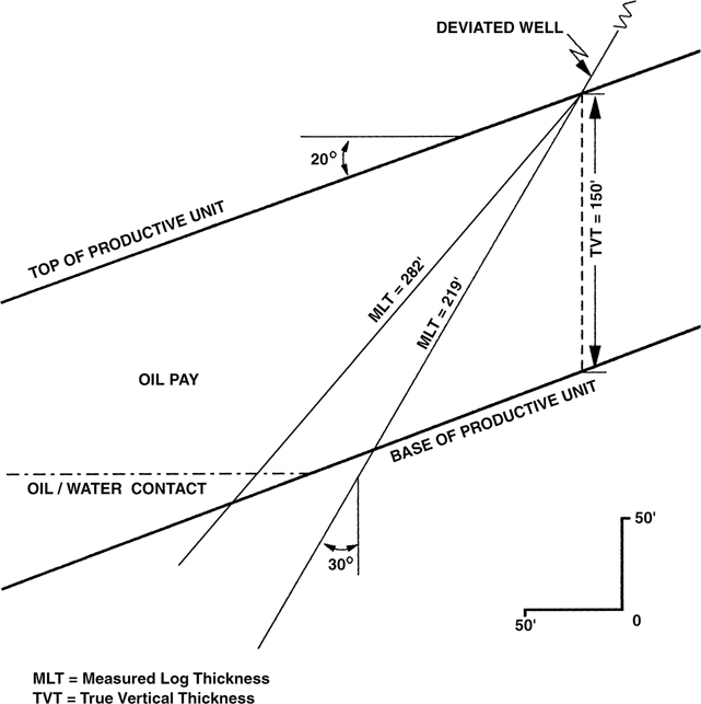
Figure 14-30 Cross section illustrates a deviated well penetrating an oil reservoir within the full-thickness area and a second deviated well penetrating the oil/water contact. See text for explanation of conversion of MLT to TVT for each well.
The well on the left in Figure 14-30 penetrates an oil/water contact. The MLT of the entire stratigraphic interval is 282 ft. What correction factor equation would you use for this MLT to calculate TVT of the oil column, at the penetration point of the top of the reservoir? In this particular situation where the penetration point is within the full-thickness area, Setchell’s equation, applied to the MLT of 282 ft, will provide the TVT of the oil at the penetration point in the top of the reservoir.
Application of Setchell’s equation to the MLT of the net oil (less than 282 ft) would result in an incorrect TVT at the penetration point in the top of the reservoir. However, if you wish to obtain the value of the vertical feet of oil directly above the penetration point of the wellbore at the oil/water contact, the use of the Setchell equation provides this value of net pay in the wedge. We will discuss this situation next.
Now consider the following situation. A well penetrates the top of an oil reservoir within the oil wedge (i.e., directly above the oil/water contact). The following data apply to the well and well log:
Wellbore deviation is 30 deg due west;
Bed dip is 20 deg due west;
MLT of net sand within the productive unit, from top to base, is 219 ft; and
MLT of net sand from the top of the unit to the oil/water contact is 115 ft.
What is the vertical thickness of the oil column under the penetration point of the well at the top of the reservoir? Draw a cross section showing the relationship of the well to the productive unit and, using Eq. (14-1), calculate the TVT of the oil under the penetration point at the top of the reservoir. Is the correct answer 150 ft, 100 ft, or 79 ft? If you calculated 150 ft, this thickness is equal to the total true vertical thickness of net sand directly under the penetration point of the well at the top of the sand (Fig. 14-30). If you calculated 79 ft, this is the vertical thickness of net oil pay directly above the point where the well penetrates the oil/water contact. A review of Figure 14-31 shows that the oil/water contact is a horizontal surface. Therefore, we do not have to consider any bed dip correction factor to calculate the net pay directly under the penetration point. No bed dip affects the TVT of the net oil sand, since the oil/water contact is a horizontal surface, and the penetration point at the top of the sand is a point directly over the oil/water contact. Therefore, Eq. (14-1), as applied to calculation of net oil sand directly beneath the penetration point of the well at the top of the sand, reduces to the correction factor for wellbore deviation multiplied by the MLT from the top of the sand to the oil/water contact, which is 115 ft. The net oil pay calculates as
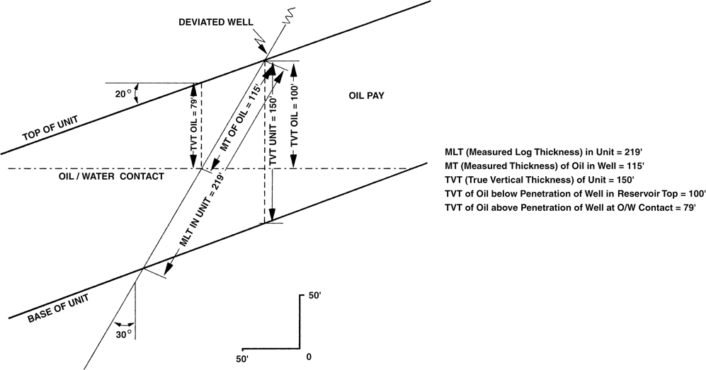
Figure 14-31 Deviated well penetrates the reservoir within the oil wedge (directly above the oil/water contact). TVT of oil column, directly below the penetration point of the well at the top of the reservoir, is calculated by simply multiplying the MLT of oil by the cosine of the wellbore deviation angle.
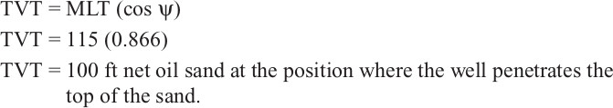
Notice the result if we consider bed dip, as well as wellbore deviation, to determine the correction factor for this case; that is, if we incorporate bed dip equal to 20 deg in Setchell’s equation, Eq. (14-1). Then we are calculating the correction factor used to determine the TVT of total net sand at the penetration point at the top of the reservoir, as well as the correction factor for the TVT of net oil sand directly above the penetration point of the well at the oil/water contact (Fig. 14-31). Calculating the correction factor (CF) in Setchell’s equation,

Using the data provided in Figure 14-30, the correction factor is based on
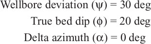
Therefore,
The true vertical thickness of the net sand at the penetration point of the well at the top of the sand is
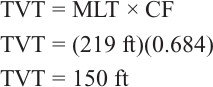
The true vertical thickness of the net oil pay sand above the penetration point of the well at the oil/water contact is
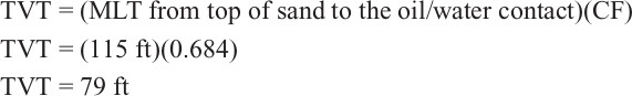
The preceding discussion shows that a fluid contact in a deviated well is a special condition for which only the correction factor for wellbore deviation may be required to convert a MLT to TVT, even though the beds are dipping at a significant angle. We make an important conclusion here: Wherever the penetration point of a well at the top of a reservoir is above a fluid contact (in the wedge), as in Figure 14-31, the dip of the beds can be considered zero in the equation for determining the net pay TVT at the penetration point at the top of the reservoir. In other words, use the simple equation TVT = MLT cos ψ. Furthermore, as shown in Figure 14-31, if the actual reservoir bed dip and the MLT of the net pay sand are used in Eq. (14-1), Setchell’s equation, then the TVT of the net pay is calculated directly above the point of penetration of the oil/water contact. Spot this point on the net oil map and use its TVT net pay value in the contouring of net oil, in addition to using the net pay value at the penetration point at the top of the reservoir.
Figure 14-32 illustrates a situation in which a reservoir containing oil and gas is penetrated by a deviated well. In this case, the vertical thicknesses of the oil and gas columns must be determined for isochore mapping. Using the data provided in the figure, verify the TVT for the oil and for the gas at two separate locations: (1) directly beneath the penetration point of the well at the top of the reservoir, and (2) the penetration point of the gas/oil contact. Finally, calculate the TVT of water, oil, and gas at the point where the well penetrates the oil/water contact (dashed line).
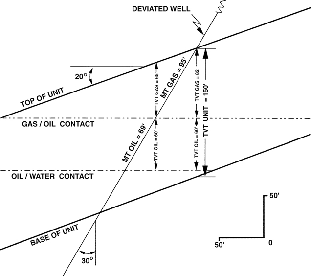
Figure 14-32 The deviated wellbore penetrates the reservoir directly above two separate fluid contacts (gas/oil and oil/water).
Figure 14-33 illustrates a well deviated in an up-dip direction, penetrating an oil reservoir in the oil wedge. The same procedures as previously discussed are used to calculate the TVT of oil at the locations where the well penetrates the top of the reservoir and the oil/water contact. If desired, the TVT of oil can also be calculated at the position where the well penetrates the base of the productive unit. First, calculate the TVT of the water column at this location, and then subtract this value from the TVT of the total net sand to arrive at the vertical thickness for oil.
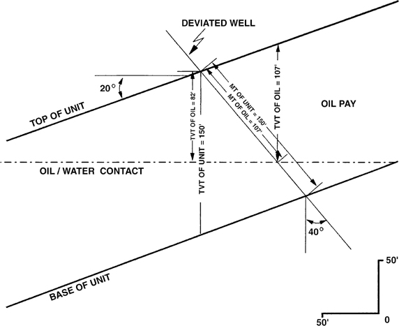
Figure 14-33 Deviated well drilled in an up-dip direction, penetrating a reservoir within the oil wedge. True vertical thickness calculation methods are the same as those for a well drilled in a down-dip direction, penetrating the top of a reservoir within the hydrocarbon wedge.
Consider the case if the well in Figure 14-33 had been drilled slightly to the right and penetrated the top of the reservoir within the wedge zone but penetrated the base of the reservoir above the oil/water contact. Use of Setchell’s equation allows calculation of the TVT of the net pay at the point where the well penetrates the base of the reservoir. If the depth of the oil/water contact is not known, the TVT of net pay at the point the well penetrates the top of the reservoir is not known, although a minimum amount of net pay can be determined by assuming the oil/water contact is immediately below the penetration point of the base of the reservoir.
If a well penetrates a reservoir up-dip of the ILW, the TVT of the pay in the well at the point of penetration of the reservoir is given by Setchell’s equation. If a well penetrates a reservoir down-dip of the ILW, the TVT of the pay in the well at the point of penetration of the reservoir is given by the vertical distance between the penetration point and the hydrocarbon/water contact.
By having a good understanding of the geometric relationship of the productive unit, wellbore, and fluid contacts, we can use this knowledge to our advantage. The calculation of the net gas or net oil at various points in a well, such as the well’s penetration point at the top of the productive unit, base of the unit, or at fluid contacts, can provide additional net pay values. These values can be used in the preparation of the net gas or net oil isochore maps, providing additional control in the wedge zones.
The detailed calculations shown in this section are not always required or justified. However, the use of these techniques may prove to be very important where detailed, accurate mapping is needed for some specific reserve estimate, development plan, enhanced recovery program, unitization, equity determination, or litigation.
Mapping the Top of Structure Versus the Top of Porosity
We discuss the effect of mapping on a structure top versus a porosity top with regard to structure mapping in Chapter 8, and here we review this special condition as it relates to net pay isochore maps. We mention in Chapter 8 that the upper portion of a reservoir unit may be composed of nonreservoir-quality rock. The terms tight zone and tight streak refer to an interval of impermeable rock. Although the top of the unit may represent the actual stratigraphically equivalent top, it does not constitute the top of reservoir-quality rock. Therefore, the structure map prepared to interpret the structure may not be useful to map and evaluate the reservoir itself.
Once the structure mapping is complete, the question arises as to whether a separate map on the top of porosity is required for accurate delineation of the reservoir and for use in the construction of net hydrocarbon isochore maps, from which estimates of reserves are made. Two parameters are considered in evaluating the importance of the nonreservoir-quality rock: (1) the thickness of the tight zone, and (2) the relief of the structure. A thick tight zone has a greater effect on ultimate reserve estimates than one that is thin. Low-relief structures introduce greater error in delineating the limits of a reservoir than steeply dipping structures, particularly if the low-relief structure contains a reservoir with bottomwater. This is true because a steeply dipping reservoir is associated with a relatively small wedge zone when compared to the total area of the reservoir.
On a low-relief structure, the wedge zone of a reservoir can represent a significant portion of the total reservoir area (Fig. 14-34). Figure 14-34a shows in map and cross-sectional views a low-relief bottomwater reservoir mapped on the top of a productive unit, which consists of nonreservoir-quality rock in the upper 75 ft. The same reservoir is mapped on the top of porosity in Figure 14-34b. The net oil isochore map prepared from each structure map is shown in Figure 14-34c. The same net pay values are assigned to each well in both isochore maps. In this case, because the reservoir is on a low-relief structure, the difference in reservoir volume between the isochore map based on the top of structure and the isochore map based on top of porosity is 637 acre-feet, or a significant overestimate of 32% (Fig. 14-34d). Consequently, the volume of recoverable hydrocarbons is overestimated by 32%.
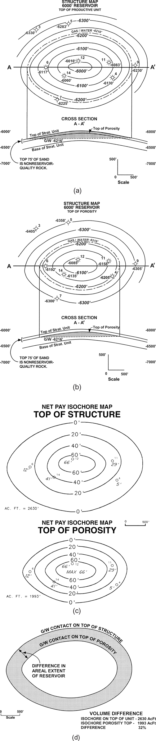
Figure 14-34 (a) The structure map on the top of the stratigraphic unit containing the 6000-ft reservoir, and the cross section A-A′. Upper 75 ft of the unit contains nonreservoir-quality rock. (b) The structure map on top of porosity (6000-ft reservoir) and the cross section A-A′. (c) Two separate net pay isochore maps: (1) the upper isochore map is based on the structure map on the top of the stratigraphic unit, and (2) the lower isochore map is based on the top-of-porosity structure map. Net pay values for all the wells are the same for each map. (d) There is a 32% reduction in reservoir volume for the net pay isochore map constructed from the top of porosity map versus the net pay isochore map constructed from the top of the stratigraphic unit. This is a significant reduction in volume.
The decision to prepare a separate map on the top of porosity, where the upper portion of a productive unit is tight, needs to be made on a reservoir-by-reservoir basis. Depending on the geometry of the reservoir and thickness of the tight zone, the difference in volume between a map on the top of the unit and one on the top of porosity may be too insignificant to warrant additional mapping.
If, for some reason, it is not possible to create a separate top-of-porosity map, it may be possible to walk wells through the wedge zone, as described earlier in this chapter. In the case illustrated by Figure 14-34, this procedure would result in a very wide zero contour, with the first net pay occurring 75 ft above the oil/water contact. Creating a separate top-of-porosity map allows you to use the BRV times net/gross method to determine the net pay. In this case, the net/gross refers to the interval from the top of the porosity to the base of the reservoir.
Fault Wedges
A fault wedge within a reservoir is defined as a wedge-shaped section of strata bounded by a fault. It is commonly just as important to map net pay within the fault wedge of a productive reservoir as it is to map net pay within the hydrocarbon wedge above water. If a productive unit is thin or the dip of the bounding fault is a high angle, the reservoir volume affected by the fault wedge may be insignificant and can be ignored for all practical purposes. In cases where the reservoir is thick or the fault dips at a low angle, the reservoir volume within the fault wedge may be significant and must therefore be included when constructing the net pay isochore map. There are several ways to handle the mapping of a fault wedge. It may be contoured in the conventional way, or a mid-trace (mid-point) method can be used.
Conventional Method for Mapping a Fault Wedge
The conventional method of contouring the fault wedge is the most accurate and should be employed whenever possible. With this method, the wedge is actually contoured using all control points in the same manner as contouring a water wedge. As with a water wedge, where the impermeable zones (shale, tight rock, etc.) are fairly evenly distributed throughout the reservoir section, the fault wedge net pay contours may be evenly spaced in the wedge zone. All the control points must be honored, however, even though it may cause an uneven spacing of the contours. Figure 14-35 shows an example of a structure map on the top of a productive unit. We use a simple, idealized map in order to provide a clear concept of mapping the fault wedge. The reservoir is bounded on the east by a west-dipping fault, with the remainder of the reservoir bounded by an oil/water contact at −8000 ft. The structure map shows the intersection of the top of the productive unit with the fault, as well as the intersection of the fault with the base of the unit (shown as a dashed line). The area between these two intersections is the area of fault wedge. In this case, the fault dips to the west at 45 deg and the productive unit dips at 30 deg. It is readily apparent from the fault intersections with the top and base of the unit that the fault wedge comprises a large portion of this reservoir. For simplicity, we assume the reservoir to have 50% net sand and 50% shale, evenly distributed throughout the gross interval. Because of this even shale distribution, we can evenly space the contours in both the hydrocarbon and fault wedges. The reservoir is in the downthrown fault block, so the control required to map the fault wedge in this example includes the intersections of the top and base of the productive unit with the fault. The upthrown trace of the fault, and therefore the fault gap as seen on a structure map, plays no part in mapping the fault wedge.
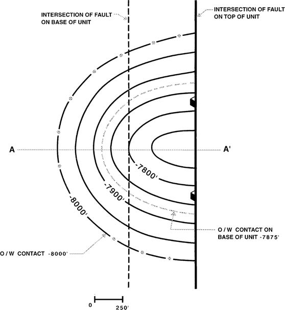
Figure 14-35 Structure map on top of a reservoir shows the intersections of a fault with the top and base of the unit. These two intersections are required in mapping the fault wedge.
Figure 14-36a illustrates the net oil isochore map for this reservoir with both the water and fault wedges conventionally contoured. The cross section A-A′, drawn below the net oil isochore map, depicts certain key control points in the reservoir, including the oil/water contact on the top of the productive unit, the inner limit of water (the oil/water contact on the base of the unit), the intersection of the base of the reservoir with the fault, and the intersection of the top of the reservoir with the fault. These key control points play an important part in the construction of the wedges for this net oil isochore map.

Figure 14-36 (a) The fault wedge is mapped using the conventional method. See cross section below map. (b) Mid-trace method for mapping the fault wedge. See cross section.
If mapping the net pay using the BRV times net/gross method, the fault surface becomes one of the bounding surfaces used in determining the BRV. If the reservoir is a bottomwater reservoir, the BRV is determined from the top of the reservoir surface, the fault surface, and the hydrocarbon/water contact. If the reservoir is an edgewater reservoir, the BRV is determined from the top of the reservoir surface, the fault surface, the hydrocarbon/water contact, and the base of the reservoir surface.
Mid-Trace Method
The use of the conventional method of contouring the fault wedge can be tedious and at times unjustified. In such cases, we can use a shortcut method for contouring the fault wedge, referred to as the mid-trace method, or mid-point method (Fig. 14-36b). To construct an isochore map using this method, first draw a line that is halfway between the intersections of the top and base of the reservoir with the fault. This line is the mid-trace. Draw the line to stop at the ILW, shown as points a and a′ in Figure 14-36b. Next, extend this line from the ILW straight to the intersection of the fault with the oil/water contact on the top of the reservoir, as indicated by a-b and a′-b′ on the figure. This line b-a-a′-b′ becomes a boundary of the reservoir. Any part of the reservoir in the fault wedge, but outside this boundary line, is considered as being folded under to convert the wedge zone inside this line to an area of full-thickness. This is illustrated in the cross section below the net oil isochore map in Figure 14-36b. Notice that this procedure extends the full-thickness area to the mid-trace. Next, extend all contours in the hydrocarbon wedge to intersect with line segments a-b and a′-b′, as illustrated in the figure. The finished map includes an enlarged full-thickness area (125 ft of net pay) plus a wedge.
Figure 14-37 illustrates the use of the mid-trace method of contouring a fault wedge with a reservoir bounded by two intersecting faults. Note that the mid-trace extension, from the inner limit of water to the intersection of the fault with the oil/water contact on the top of the unit, is in opposite directions on the individual fault wedges. Remember, always draw a line from the mid-trace to the intersection of the zero net pay contour with the fault.
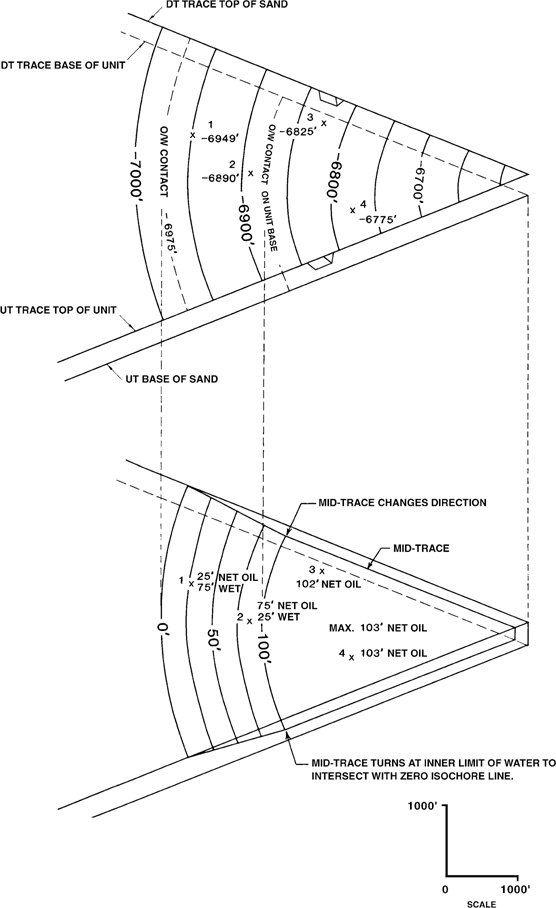
Figure 14-37 Construction of two fault wedges involving intersecting faults. Note the change in direction of the mid-traces at the inner limit of water.
It should be pointed out that Figures 14-36 and 14-37 are drawn to illustrate the mid-trace method. The fault shape implied by the fault traces (see Figs. 7-42b and 8-54b) in these figures is unlikely to occur in normal geological settings.
Nonsealing Faults
Although faults play a very important role in the trapping of hydrocarbons, studies have shown that some faults are nonsealing, thereby permitting the migration of hydrocarbons from one fault block to the next. One of the most common situations resulting in a nonsealing fault is the juxtaposition of permeable stratigraphic units across a fault, with capillary properties of the fault zone being insufficient to create a seal. This can occur where a fault does not have sufficient displacement to separate an entire permeable unit from one fault block to the next, or where juxtaposition of different permeable units exists. The concept of sealing and nonsealing faults is discussed at more length in Chapter 6.
Hydrocarbon accumulations can occur on both sides of a nonsealing fault if a trap exists in the up-structure fault block. The accumulations would have a common water level. With nonsealing faults, it is important to map fault wedges because they can contain significant amounts of hydrocarbons. We contour the fault wedge basically the same as presented in the previous section, with one exception. Since there is hydrocarbon pay upthrown and downthrown to the fault, two reservoirs and two fault wedges must be mapped to account for all the hydrocarbon volume. The isochore maps for the two reservoirs can be constructed individually or contoured as one map.
Figures 14-38 and 14-39 illustrate an example of reservoirs juxtaposed across a nonsealing fault. A productive sandstone unit contains two fault-separated reservoirs on the southern flank of a salt structure. Figure 14-38a shows the structure map on the top of porosity in Reservoirs A and B. The reservoirs are limited to the north by a vertical salt face, to the east and west by faults, and in the down-dip direction by a common gas/water contact at −10,550 ft. The interval from top to base is in excess of 200 ft thick, and it is all reservoir-quality sand. Fault B, with a vertical separation of 200 ft, has insufficient displacement to completely separate the sand, so part of the sand is juxtaposed across the fault. The same gas/water contact in both Reservoirs A and B indicates that the fault is nonsealing and that the two reservoirs are in communication. Figure 14-38b through d are the structure map on the base of the 9500-ft Sand, the fault surface map, and the net sand map respectively. These maps are required for isochore construction.

Figure 14-38 (a) Structure map on top of Reservoirs A and B. Salt face is vertical at this depth.(b) Structure map on base of Reservoirs A and B. (c) Fault surface map of Faults A and B. (d) Net sand isochore map for 9500-ft Sand.
The net gas isochore maps for the Reservoirs A and B can be constructed separately or as one single net gas isochore map. Figure 14-39a and b show the individually constructed net gas isochore maps for Reservoirs A and B respectively. Notice that the fault wedges for Faults A and B comprise a significant portion of each of the reservoirs. Figure 14-39c illustrates how the two reservoirs can be mapped together by combining the wedges for Fault B. Cross section A-A′ shows about 75 ft of sand juxtaposed across the fault at this position in the reservoir.
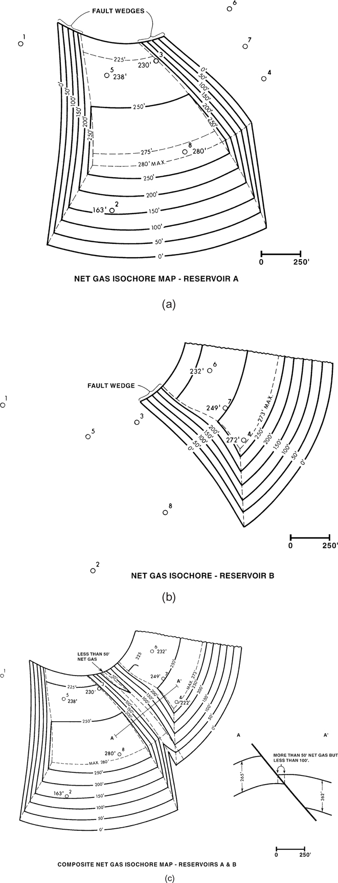
Figure 14-39 (a) Net gas isochore map for Reservoir A. The map includes two fault wedges and a water wedge. (b) Net gas isochore map for Reservoir B. Fault wedge and water wedge are significant portions of the reservoir volume. (c) Composite net gas isochore map for Reservoirs A and B. Notice the complexity in the mapping of the two fault wedges created by Fault B when both reservoirs are mapped together.
Isochore maps in which the fault wedges are combined, such as the one shown in Figure 14-39c, are difficult to construct and can easily result in errors. We recommend for simplicity of construction and planimetering that, even with nonsealing faults, each reservoir and fault wedge be mapped separately, as shown in Figure 14-39a and b. Constructing net pay isochore maps for each productive fault block can also be important in developing field development plans, as even nonsealing faults can act as baffles during production time scales. Thus, a well in one fault block may not access reserves in an adjacent fault block, even if the intervening fault is nonsealing and the two fault blocks share a common water level.
Volumetric Configuration of a Reservoir
We use a net pay map to determine the volume of a reservoir, so we want to consider how this volume, as depicted by the map, corresponds to the actual structural configuration of the reservoir. Figure 14-40 relates the net pay map depiction of volume of a gas-on-oil accumulation to the structural configuration of the productive unit. The cross section in the center of the figure shows the actual structural configurations of the oil reservoir and the gas reservoir. The cross sections in the lower portion of the figure show the varying thickness of each reservoir, with each represented as a polygon with a flat base. If we consider possible changes in thickness in the third dimension, then each polygon represents an irregular solid that has a volume equal to that of the reservoir. It is important to notice that the depicted volume is not a true representation of the structural configuration of the reservoir. The reservoir has been artificially flattened, or piled up (referred to as isochore piling), to represent the same volume that exists within the structure. The net pay map will be planimetered, and then the depicted volumetric solid is used in the calculation of the reservoir volume.
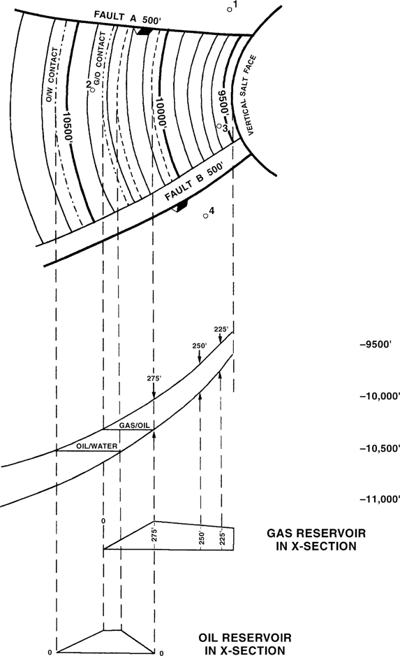
Figure 14-40 In the preparation of a net hydrocarbon isochore map, the configuration of the reservoir is completely rearranged and the base is artificially flattened. Compare the configuration of the net gas and net oil cross sections in the lower portion of the figure to that of the structure cross section in the center.
Reservoir Volume Determinations From Isochore Maps
Two methods are commonly used to determine reservoir volume from net pay isochore maps using a mechanical planimeter, the horizontal slice method and the vertical slice method. Previous editions of this book describe these methods in significant detail (Tearpock and Bischke 1991, 2003). Mechanical planimeters are rarely used today. Most reservoir volumes are calculated by digitizing maps using a planimetering program or are calculated within the software that created the maps. Individuals interested in calculating reservoir volumes using mechanical planimeters are referred to the earlier editions of this book.
Tilted Hydrocarbon/Water Contacts
So far in this chapter, we have assumed that hydrocarbon/water contacts are flat. This is an excellent assumption and accurate in most cases, but there are exceptions. Hubbert (1953) recognized that hydrodynamic flow in an aquifer causes a hydrocarbon/water contact to tilt in the direction of flow. A comprehensive discussion of tilted hydrocarbon/water contacts is beyond the scope of this book, but a basic introduction to the concept is worthwhile because of the potential impact on net pay isochore mapping.
The inclination of hydrocarbon/water contacts is described by the following equation (Hubbert 1953):
where

Equation (14-2) shows that for any given hydraulic head, the inclination of the hydrocarbon/water contact is a function of the density difference between the hydrocarbon and water. The greater the density difference, the less the tilt on the contact. Lower-gravity, higher-density oil in an aquifer of fresh water will have a greater inclination in the hydrocarbon/water contact than a high-gravity, lower-density oil in an aquifer of high-salinity water for any given hydraulic head. Gas/water contacts show even less inclination for a given hydrodynamic head because of the greater density difference in the two fluids.
Tilted hydrocarbon contacts are not caused by the viscous drag of aquifer water on trapped hydrocarbons. They are caused by pressure gradients, or technically hydraulic potential gradients, within the reservoir. Both inclined contacts and aquifer flow are responses to the same force but do not cause each other.
Most cases of hydrodynamic flow are driven by elevation differences between the recharge area of an aquifer and its eventual discharge region. In the case of the U.S. Gulf Coast, the hydraulic head of shallow, low-salinity aquifers may be two or three feet per mile (Hubbert 1953). In the U.S. Great Plains, the hydraulic head may be ten feet per mile, whereas in intermontane basins, the hydraulic head may be hundreds of feet per mile (Hubbert 1953). The greater the hydraulic head, the greater the inclination of the hydrocarbon/water contact for a given density contrast between hydrocarbons and aquifer water. For gases, ρw/(ρw – ρh) is between one and two, so a gas/water contact is typically inclined between one and two times the hydraulic gradient. Thus, an aquifer gradient of 10 ft/mi would result in an inclined gas/water contact of between 10 and 20 ft/mi (Hubbert 1953). For oils, the term ρw/(ρw – ρh) ranges from two to infinity but is generally between seven and fifteen with ten being a reasonable average number (Hubbert 1953).
Many aquifers are hydrodynamic. If the formation water is fresh, it must be hydrodynamic, and a hydrocarbon/water contact will be tilted (Hubbert 1953). If formation water is saline, it may be flowing (hydrodynamic), and a hydrocarbon/water contact will be tilted; or the formation water may be static, and the hydrocarbon/water contact will be horizontal. Most hydrodynamic aquifers are onshore and associated with significant topographic relief. Work in the North Sea, however, suggests that some deep, offshore aquifers are hydrodynamic due to dewatering of overpressured shales into laterally extensive permeable units that subcrop normally pressured permeable units (Dennis et al. 2000).
Even in areas with hydrodynamic flow, the inclination on an oil/water contact may be small, a maximum of a foot or two from one side of the accumulation to another. Small inclinations on oil/water contacts can be very difficult to resolve from uncertainties in depth measurements, as discussed in Chapter 3. For a very large field covering several miles laterally, however, the same inclination of the contact can result in tens of feet of elevation difference from across the field in the direction of hydrodynamic flow (Dennis et al. 2000). The inclination of the contact can be differentiated conclusively from depth measurement uncertainties if good-quality formation pressure is available (Fig. 14-41).

Figure 14-41 Formation pressures for Pierce Field in the central North Sea. Pierce Field is associated with two salt domes and has two separate culminations with two separate gas caps with different gas/water contacts. All of the oil lies on a single pressure gradient. Aquifer pressures on different sides of the field have similar gradients but are slightly offset from one another with the aquifer pressure at a constant depth decreasing from east to west. The oil/water contact at Pierce Field dips to the west at about 5 deg, or almost 500 ft/mi (90 m/km). (Modified from Dennis et al. 2000. Published with permission from Norwegian Petroleum Society.)
Oil fields with gas caps in hydrodynamic units behave differently depending on how much inclination there is on the oil/water contact. In a hydrostatic environment, both the gas/oil contact and the oil/water contact in an oil field are horizontal (Fig. 14-42a). If the oil/water contact is inclined such that the gas cap is still underlain everywhere by oil, the oil/water contact is inclined but the gas/oil contact is horizontal. This is because the oil is in contact with the hydrodynamic aquifer, whereas the gas is only in contact with the hydrostatic oil (Fig. 14-42b). If the oil/water contact is inclined further, part of the gas cap may be underlain by the hydrodynamic aquifer. It this case, the gas/oil contact will be horizontal but the gas/water contact will be inclined, although less so than the oil/water contact (Fig. 14-42c). Finally, if the oil/water contact is sufficiently inclined, the oil accumulation may be totally separated from the gas cap, so that the gas will be underlain everywhere by water and the gas/water contact will be inclined (Fig. 14-42d).
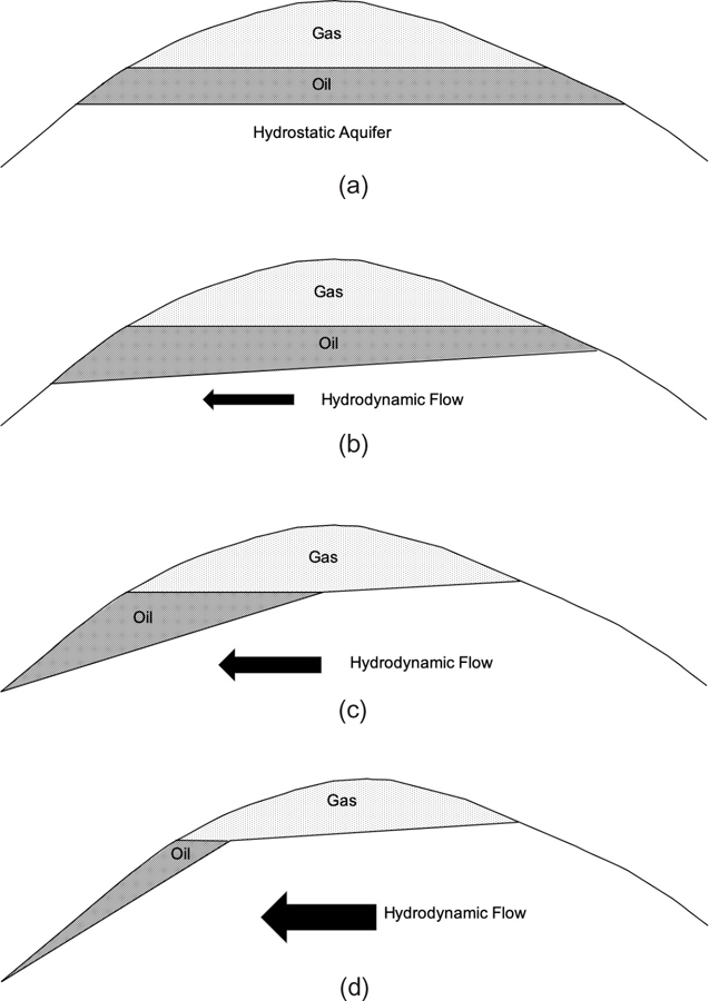
Figure 14-42 (a) Oil field with a gas cap in a hydrostatic aquifer. Both the gas/oil and oil/water contacts are horizontal. (b) Oil field with a gas cap in a hydrodynamic aquifer with a small hydraulic head. The oil/water contact is inclined, as the oil is in contact with the hydrodynamic aquifer. The gas/oil contact is horizontal, as the gas is only in contact with the hydrostatic oil. (c) Oil field with a gas cap in a hydrodynamic aquifer that has a moderate hydraulic head. The oil column has been inclined sufficiently that part of the gas cap is underlain by hydrostatic oil and part of the gas cap is underlain by hydrodynamic water. The gas/oil contact is horizontal and the gas/water contact is slightly inclined. (d) Oil field with a gas gap in a hydrodynamic aquifer with a significant hydraulic head. The oil column has been inclined to the point that it is almost completely separated from the gas cap. The oil/water contact is strongly inclined, and most of the gas/water contact is inclined. (Modified from Hubbert 1953. Published by permission of J. Brenneke.)
To properly calculate the volumetrics of an oil field, it is important to distinguish inclined hydrocarbon/water contacts from perched hydrocarbon/water contacts because inclined contacts tend to have much greater impact on net pay volumes than do perched contacts. Both cases have hydrocarbon/water contacts at different elevations in different parts of the field. In both cases, reservoir formation pressures of the hydrocarbon phase will lie on a single line, reflecting the in situ density of the hydrocarbon. The water pressures will intersect the hydrocarbon pressure line at various depths, reflecting the different oil/water contacts (compare Figs. 8-86 and 14-41). One key difference is that perched contacts can occur only in edge water reservoirs. A second difference is that perched contacts are associated with closed lows on the base of the reservoir, whereas tilted contacts are not. For perched water to be an acceptable explanation, you must be able to map a closed low on the base of the reservoir. A third difference is that the chemistry of the formation water beneath a perched contact may be significantly different that the chemistry of the main aquifer, whereas there are not significant differences in formation water chemistry in hydrodynamic reservoirs over short distances, although there may be chemistry trends on a basinal scale (e.g., Bond 1972).
Hydrocarbon/water contacts at slightly different depths may reflect actual different contacts, or they may reflect difference in depth measurements or uncertainties in directional surveys (see Chapter 3). Much of this uncertainty can be clarified if reservoir pressures are available, as discussed in Chapter 3 (Fig. 3-27). One additional uncertainty is in the measurement of reservoir pressures (Fig. 14-43). Very small pressure differences may be due to gauge differences in the repeat formation tester (RFT) tools.
Figure 14-43 Repeat formation test pressures from two gauges (triangle and circle) in a single wireline tool in a deep water Gulf of Mexico well. As the two gauges were made up into a single tool, their relative depth is known. The difference between the two gauges is a measure of the accuracy of the gauges. The difference between the gauges, about 6 psia, is 0.03% of the pressure measurement, well within the specs quoted by the service provider. The single star is a logging-while-drilling (LWD) pressure from the same well that has been depth-shifted to tie the log measurements. The difference between the LWD pressure and the wireline pressures, again about 0.03% of the total gauge pressure, may be due to differences in gauges, or it may be due to differences in tool design and operation. (Published by permission of J. Brenneke.)
Tilted hydrocarbon/water contacts can affect both bottomwater and edgewater reservoirs. The procedure for mapping net pay for reservoirs with inclined hydrocarbon/water contacts is very similar to mapping net pay for reservoirs with horizontal contacts. With inclined contacts, the zero net pay contour does not track a structure contour, and the isochore contours may not be as similar in shape to structure contours as they would be if the contact were horizontal. If mapping these reservoirs on a computer, the only difference is that hydrocarbon/water surface used in the gross reservoir determination is not horizontal.
Introductory Reservoir Engineering
Reservoir engineering must be involved in all phases of oil and gas prospect evaluation from the initial phases of exploration through field development. Prior to any wells being drilled on a prospect, the most likely reservoir engineering parameters must be assumed in a preliminary evaluation to estimate the potential hydrocarbons. Initial drilling provides basic reservoir parameters, but offset information from analogous fields is used to predict the performance of the new discovery. Finally, during the field’s productive life, performance data needs to be constantly evaluated to allow revisions to the original assumptions and to develop and modify the field’s depletion plan. The last phase is especially critical to optimize drainage of recoverable reserves yielding maximum productivity and revenue.
An excellent review of the history of reservoir engineering is found in Craft and Hawkins (1959). One of the major benefits to the geologist of becoming familiar with basic reservoir engineering is to understand what a reservoir engineer requires for the evaluation of hydrocarbon reserves. A list of the symbols, nomenclature, and other pertinent information adopted by the Society of Petroleum Engineers for use in reservoir engineering can be found at the Society’s website (www.spe.org). It is essential for a geologist to become familiar with the basics of petroleum engineering and to work closely with the petroleum engineer to obtain the necessary data to evaluate hydrocarbon reserves.
Reservoir Characterization
After the identification of hydrocarbons in a permeable stratigraphic unit, a plan must be established to estimate the in-place volumes of these hydrocarbons and what might be expected to be recovered. Recoverable hydrocarbons are referred to as hydrocarbon reserves. Because the productive characteristics of a reservoir or field may not be fully known until it is maturely developed, offset analogous reservoirs need to be considered as models to the development of any new discovery. With a model to follow, various reservoir-engineering parameters such as reservoir porosity, permeability, and water saturation can be estimated to allow volumetric analyses of the reservoir or field to estimate potentially recoverable reserves.
Estimation of Reserves
Reservoir net volume is calculated from net hydrocarbon isochore maps, as earlier discussed in this chapter. From detailed log analysis, rock properties can be identified. As an example, interstitial water saturation must be estimated for reserve determinations. Detailed reservoir petrophysics for use in calculating reserves is beyond the scope of this book; however, a presentation of general reservoir engineering may be helpful, and it is outlined here.
Using the letter symbols G and N, initial in-place volumes of gas and oil can be determined by the following equations.
and
where
Gas Reservoirs.
Equation (14-3) is used to estimate original gas-in-place. There are several unknown factors in the equation that must be determined. The formation volume factor (FVF) or Bgi is defined as the relationship of gas volumes from surface conditions to reservoir conditions. For gas reservoirs, Bgi is expressed in standard cubic feet per reservoir cubic foot, SCF/cu ft. As defined here, Bgi is greater than 1 as gas expands from reservoir conditions to standard conditions, which approximate surface conditions. Bgi can also be defined as reservoir cu ft/standard cu ft. In that case, Bgi is less than 1 and moves from the numerator to the denominator in Eq. (14-3), and Eq. (14-3) becomes directly analogous to Eq. (14-4). The porosity is expressed as a fraction of the net volume, and the interstitial water (Swi) is a fraction of the pore volume.
To determine the unit recovery for a gas reservoir, the final reserve volume per acre-foot is determined on the basis of the reservoir drive mechanism. This fractional recovery, or recovery factor, represents the difference between the initial unit-in-place gas and the final, or abandonment, unit-in-place gas.
or

where

This recovery factor is indicative of depletion drive reservoirs, where interstitial water saturation remains unchanged and, conversely, gas saturation remains constant. The other end of the spectrum with regard to drive mechanisms is a strong water drive, where produced gas is being replaced by encroaching water (there is no appreciable pressure loss and Bgi = Bga). The recovery factor for a water-drive gas reservoir, which is representative of the change in gas and water saturations in the reservoir due to production, is shown in Eq. (14-6).

where
Oil Reservoirs. Oil reservoirs are often more difficult to analyze for a number of reasons, including the presence in some reservoirs of both oil and gas. If an oil reservoir is found without free gas, the oil is said to be undersaturated. An oil reservoir with a free gas cap is indicative of a saturated oil reservoir.
Equation (14-4) is used to volumetrically determine original oil-in-place. The variables in Eq. (14-4) are very similar to those discussed for Eq. (14-3). If we consider an undersaturated oil reservoir under a strong water drive, the recovery factor is based on the following equation.

where
Where there is an initial gas cap, the oil is saturated. In such cases, the reservoir can be produced under drive mechanisms other than water drive. These include dissolved gas, gas cap, or a combination drive. The opposite end of the recovery factor spectrum from a water drive reservoir is that of a dissolved gas drive reservoir.

where
Field Production History
Once reservoir or field production has been established and sufficient quantities of hydrocarbons produced, performance data can be used to estimate original and remaining reserves, and to forecast future performance. It is good practice to monitor both production and reservoir pressure data. These points of reference are invaluable in evaluating reservoir heterogeneities and are applicable to material balance equations.
Various performance curves can be used to evaluate reserves and forecast future production trends. The most common performance curves are those which plot the production of oil, gas, and water versus time. In many instances, performance evaluation is by far the most accurate method for estimating the original in-place volume of hydrocarbons, estimating recoverable reserves, and forecasting future performance. The following is a partial list of the types of performance curves that can be plotted.
Monthly production (oil or gas) versus time
Flowing tubing pressure versus time
Bottom-hole pressure data versus cumulative production
Percent oil cut versus cumulative production
Water yield versus cumulative gas production
A detailed discussion of these performance curves is beyond the scope of this book. We again refer you to Craft and Hawkins (1959).
Interval Isopach Maps
As discussed in the beginning of this chapter, an isopach map is one in which the true stratigraphic thickness of a single stratigraphic interval is contoured, such as a stratigraphic unit or an interval between two stratigraphic markers. Such a map is referred to as an interval isopach map. Interval isopach maps are particularly useful in determining the history of movement along faults and of development of growth structures, such as salt dome structures and folds, as well as being useful in the interpretation of depositional environments and paleostructures.
The full application of interval isopach maps is beyond the scope of this text. More specifically, we address the determination and use of the proper interval thicknesses obtained from well logs or seismic data to be used for construction of interval isopach maps. Interval isopach maps reveal the true stratigraphic thicknesses of units rather than vertical thicknesses. The TST is the thickness measured perpendicular to the top and base of the stratigraphic interval. Where strata have no dip or have only gentle dips, TST equals or approximates TVT. But with increasing dip, the differences become substantial and a correction factor is applied to TVT to obtain TST. The relationship is given as
where
For example, with a 10-deg bed dip, an interval with a TST of 100 ft has a vertical thickness of 101.5 ft; at a 20-deg dip, the vertical thickness is 106.5 ft. At a 45-deg dip, however, the vertical thickness becomes 141 ft, which is significantly different than the stratigraphic thickness. If the TVT is the value contoured, the map is more correctly referred to as an isochore map. Therefore, net sand and net pay maps are isochore maps.
True Stratigraphic Thickness from Well Logs
The determination of stratigraphic thickness from well logs presents a few complications. In areas of nearly flat-lying beds, the TVT approximates TST. The determination of stratigraphic thickness does, however, become more complicated around steeply dipping structures. Figure 14-44 shows the effect of changing bed dip on vertical well log thickness of a stratigraphic unit whose TST is constant. With zero bed dip, TVT equals TST. At a 20-deg bed dip, the TVT is only 1.06 times TST. At a 40-deg bed dip, the TVT is equal to 1.30 times TST, and at 60 deg, the TVT is twice as thick as the TST. Assuming vertical wells, if the upper and lower markers chosen for interval isopaching are parallel or nearly so (that is, they are at or near the same dip), Eq. (14-9) can be used to convert vertical thickness to stratigraphic thickness.
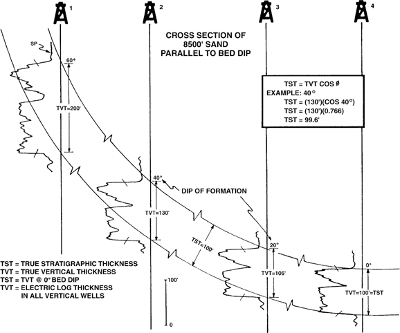
Figure 14-44 Effect of changing bed dip on TVT of a stratigraphic unit, where TST is constant.
If the thickness of the interval changes, and thus the dips of the upper and lower surfaces of the interval are different, then the correction factor based on the cosine of a single bed dip, either at the upper surface or lower surface, will not be accurate. For such cases, another equation is required (Tearpock and Harris 1987).
where
Figure 14-45 shows the equation and an example problem. This equation takes into account the dip of the upper and lower surfaces and the vertical thickness of the interval.
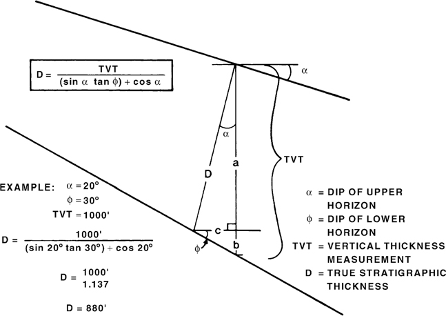
Figure 14-45 Cross section showing the geometric relationship between two horizons that have different angles of dip. Eq. (14-10) is used in this type of situation to convert TVT to TST. (Prepared by C. Harmon. Modified from Tearpock and Harris 1987. Published by permission of Tenneco Oil Company.)
Finally, in the case of deviated wells, the measured log thickness must be first corrected to TVT, and then corrected to TST. The procedure for vertical thickness conversions is discussed in this chapter and in Chapter 4.
To avoid making laborious stratigraphic thickness calculations, the graph in Figure 14-46 can be used to calculate TST if the vertical thickness and the dips of the upper and lower surfaces are known. The horizontal axis represents the dip of the upper surface, and the vertical axis represents the correction factor. The curves within the graph represent the values obtained by subtracting the dip of the upper surface from the dip of the lower surface (note positive and negative values). Consider the following example.
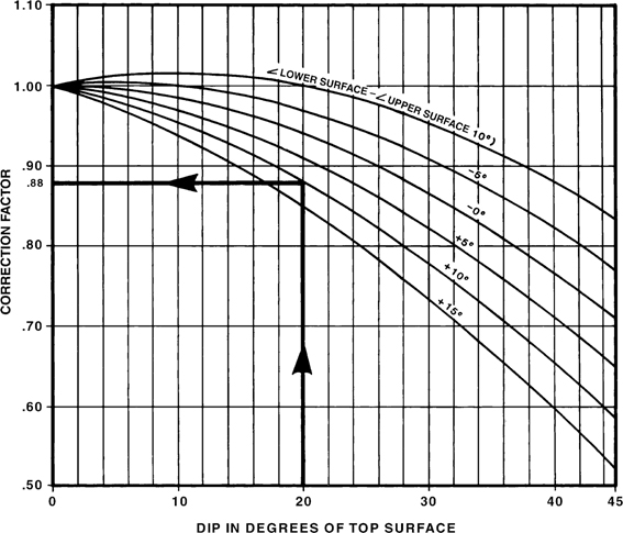
Figure 14-46 Graph derived from Eq. (14-10) and used to determine the correction factor for converting TVT of a stratigraphic interval to TST, where the upper and lower surfaces dip at different angles. (Prepared by C. Harmon. From Tearpock and Harris 1987. Published by permission of Tenneco Oil Company.)
Data:

To use the graph, first subtract the dip of the upper surface from the lower surface. This value determines which of the curved lines to use for the correction factor.
Enter the graph on the horizontal axis at 20 deg and project vertically until the line intersects the curve with value equal to the dip of the lower surface minus the dip of the upper surface. In this case, it is the +10-deg curve.
From the intersection with the curve, project horizontally to the left to intersect the vertical axis and determine the correction factor. In this case, it is 0.88.
Therefore,
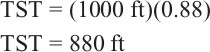
Interval Isopach Construction Using Seismic Data
Using seismic data for interval isopach construction can give you many additional data points between well control. In areas of relatively low dip (10 deg or less) and parallel horizons, the TVT calculated from seismic is a close approximation of the TST. If you have seismic data that has been converted to depth, the process is straightforward. If the seismic data is in time, the procedure in this type of area is almost as straightforward: The time-converted depth of the upper horizon is subtracted from the time-converted depth of the lower horizon to arrive at an interval thickness. The basic requirement is an accurate time–depth function.
In areas of steeper dip and nonparallel horizons, you should be aware of some visual pitfalls inherent in time seismic sections. The basic point to remember is that a time section is not a cross section. It is distorted due to the two very different dimensions displayed on a section: time along the vertical axis and distance along the horizontal axis. These dimensional differences often introduce some very pronounced vertical exaggeration.
To illustrate this, observe the two horizons indicated in Figure 14-47a. They obviously diverge from one another as the interval thickens into a fault. How do we determine the TST of the interval? The first inclination is to draw a perpendicular line, shown as A on the figure, from the top horizon to intersect the bottom horizon, and calculate trigonometrically the stratigraphic thickness using the time-converted depths at both points, along with the lateral distance between the two points. THIS IS WRONG.
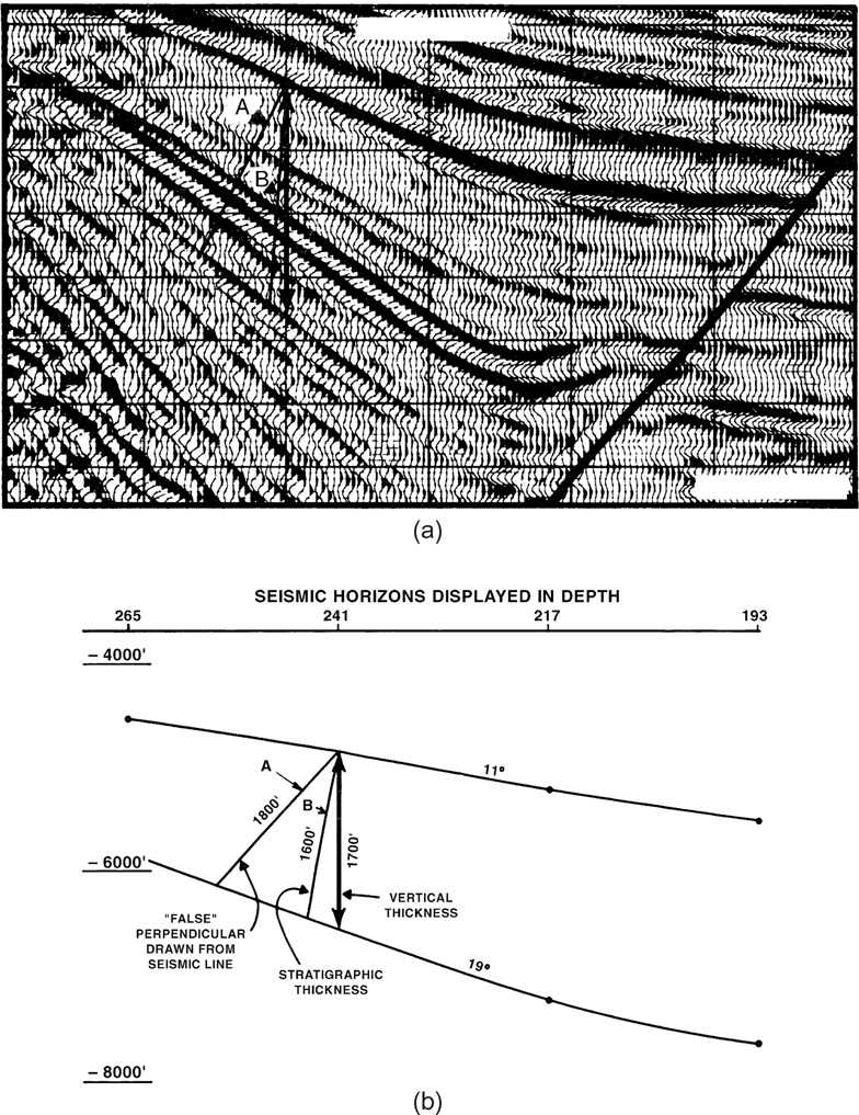
Figure 14-47 (a) Which line, A or B, represents the true stratigraphic thickness of the designated interval? (b) True (1:1 scale) cross section of the seismic interval shown in (a). (Prepared by C. Harmon. From Tearpock and Harris 1987. Published by permission of Tenneco Oil Company.)
To see graphically what is actually present, look at Figure 14-47b, which shows the horizons converted to depth and displayed at a true 1:1 scale. Line A, drawn earlier as perpendicular to the top horizon on the seismic line, is in fact a longer segment than the true perpendicular, which is line B on the seismic line and cross section. The reason for this pitfall is that the time seismic line, at this depth, has about a 2:1 vertical exaggeration. In this case, you would post a larger thickness for the interval than is actually present. To obtain corrected data points, you need to apply Eq. (14-10), which uses the dip of the top and bottom horizons, and the vertical thickness of the interval. The graph in Figure 14-46 can also be used to determine the stratigraphic thickness.
In summary, seismic information can be a valuable source of interval thickness data, as long as you are aware of the visual distortion inherent in time seismic data and properly account for it in the calculation of stratigraphic thicknesses.