
Chapter 6
Point Operations
Beginning with this chapter, the focus is on how specific image processing operations may be implemented on an FPGA. The next few chapters describe preprocessing and other low level operations. Later chapters move to intermediate level operations.
An assumption in the next few chapters (unless stated otherwise) is that the ![]() -bit pixels represent unsigned values from 0 to
-bit pixels represent unsigned values from 0 to ![]() . Most of the examples here will be given with
. Most of the examples here will be given with ![]() bits.
bits.
6.1 Point Operations on a Single Image
The simplest class of image processing operations is that of point operations. They are so named because the output value for a pixel depends only on the corresponding pixel value of the input image:
where ![]() is some arbitrary function. Since the output value depends only on the input value and not on the location of the pixel in the image, point operations may be represented by a mapping or transfer function, as shown in Figure 6.1.
is some arbitrary function. Since the output value depends only on the input value and not on the location of the pixel in the image, point operations may be represented by a mapping or transfer function, as shown in Figure 6.1.
Figure 6.1 A point operation maps the input pixel value, ![]() , to the output value,
, to the output value, ![]() , via an arbitrary mapping function,
, via an arbitrary mapping function, ![]() . Right: implementation of a point operation using stream processing.
. Right: implementation of a point operation using stream processing.
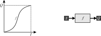
From a hardware implementation perspective, point operations may be easily implemented in any processing mode. However, because each operation is applied exactly once to each pixel in the image, the simplest approach is to systematically pass each input pixel through a single hardware block implementing the function. This corresponds to the streamed mode of processing and is illustrated in the right panel of Figure 6.1. Since each pixel is processed independently, point operations can also be easily implemented in parallel. The image may be partitioned and a separate processor used with each partition.
In spite of their simplicity, point operations have wide use in terms of contrast enhancement, segmentation, colour filtering, change detection, masking and many other applications.
If the subsequent imaging operation requires random access of pixels (for example from a frame buffer), the hardware block implementing the point operation may be placed between the source and subsequent operation. In this way, as the pixels are read, they are transformed by the point operation as required for the subsequent process.
6.1.1 Contrast and Brightness Adjustment
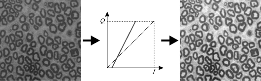
One interpretation of the mapping function is to consider its effect on the brightness and contrast of the image. To make an image brighter, the output pixel value needs to be increased. This may be accomplished by adding a constant, as illustrated in Figure 6.2. Similarly, an image may be made darker by decreasing the pixel value, which may be accomplished by subtracting a constant. In practise, adjusting the brightness is more complicated than this because the human visual system is nonlinear and does not consider each point in an image in isolation but relative to its context within the overall image. This is shown in the optical illusion in Figure 6.3, where the band through the image appears brighter on the left and darker on the right (actually the pixel value is the same).
Figure 6.2 Increasing the brightness of an image by adding a constant.
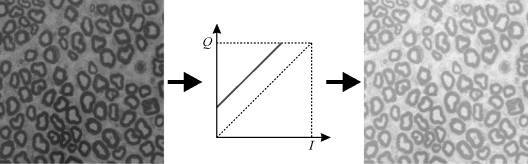
Figure 6.3 Brightness illusion.

The contrast of an image is affected or adjusted by the slope of the mapping function. A slope greater than one corresponds to an increase in the contrast (Figure 6.4) and a slope less than one corresponds to a contrast reduction. This may be accomplished by multiplying by a constant greater than or less than one respectively.
Figure 6.4 Increasing the contrast of the image.
A relatively simple point operation for adjusting both the brightness and contrast is:
where ![]() and
and ![]() are arbitrary constants that control the brightness and contrast. One issue is what to do when the value for
are arbitrary constants that control the brightness and contrast. One issue is what to do when the value for ![]() exceeds the range of representable values. For example, with an eight bit per pixel representation, what should be output if
exceeds the range of representable values. For example, with an eight bit per pixel representation, what should be output if ![]() is outside the range of 0–255? The default of just taking the eight least significant bits and ignoring any overflow would cause values outside this range to wrap around. If the goal is to enhance the brightness or contrast of an image, this is seldom the desired effect. More sensible would be for the output to saturate or clip to the limits. Note that clipping the output is not invertible.
is outside the range of 0–255? The default of just taking the eight least significant bits and ignoring any overflow would cause values outside this range to wrap around. If the goal is to enhance the brightness or contrast of an image, this is seldom the desired effect. More sensible would be for the output to saturate or clip to the limits. Note that clipping the output is not invertible.
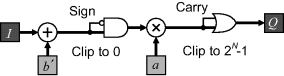
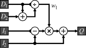
Clipping requires building hardware to detect when the limits are exceeded and adjust the output accordingly. This is shown in block diagram form in Figure 6.5. Note that either the brightness or contrast operation may be performed first depending on the form of Equation 6.2.
Figure 6.5 Schematic representation of a simple contrast enhancement operation. Right: improving the performance by moving the comparisons to the input.
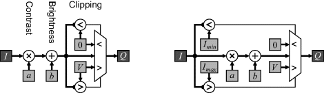
On the left in Figure 6.5, the clipping tests are performed after the calculation of Equation 6.2. This means the propagation delay for the complete operation includes the time required for the clipping test. If, however, the clipping test was performed on the input, it would be computed in parallel with the contrast enhancement operation (as shown on the right), and the propagation delay would be reduced. The clip limits referred to the input are:
(6.3) ![]()
This form is most practical if the gain and offset values are constant, so that the input range can be determined at compile time.
This circuit may be further simplified by relying on the fact ![]() . With positive gain, it is only the offset that can cause the result to go negative. Using the second form of Equation 6.2, the sign bit of the addition can be used to set the output to zero. Similarly, the carry from the multiplication can be used to clip to the maximum by setting all the bits to one. This scheme is shown in Figure 6.6.
. With positive gain, it is only the offset that can cause the result to go negative. Using the second form of Equation 6.2, the sign bit of the addition can be used to set the output to zero. Similarly, the carry from the multiplication can be used to clip to the maximum by setting all the bits to one. This scheme is shown in Figure 6.6.
Figure 6.6 Simplified circuit. The sign bit from the addition sets the result to zero if the number is negative, and the carry from the multiplication sets the result to all ones.
Further optimisations may be made. Obviously if the gain and offset are constant then the multiplication may be replaced by a series of fixed additions. Representing the gain in canonical signed digit form will reduce the number of terms that need to be added.
A common contrast enhancement method is to derive the gain and offset from the minimum and maximum values available in the input image. The contrast is then maximised by stretching the pixel values to occupy the full range of available pixel values. This obviously requires that the whole image be read to determine the extreme pixel values, with consequent timing issues. Such issues are discussed in Section 7.1.2 with histogram equalisation, another adaptive contrast enhancement technique.
A contrast reversal is obtained if the slope of the transfer function is negative. For example to invert the image, a gain of −1 is used, as shown in Figure 6.7, where:
Figure 6.7 Inverting an image (Photo courtesy of Robyn Bailey).
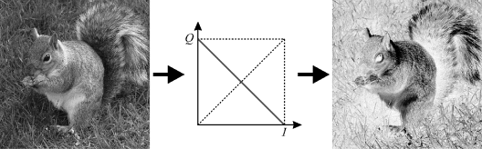
(6.4) ![]()
Logically, this may be obtained by taking the one's complement (inverting each bit) of the input.
The transformation does not necessarily have to be linear. The same principle applies with a nonlinear mapping: raising or lowering the output will increase or decrease the brightness of the corresponding pixels; slopes greater than one correspond to a local increase in contrast, while slopes less than one correspond to a decrease in contrast; a negative slope will result in contrast inversion. A nonlinear mapping allows different effects at different intensities.
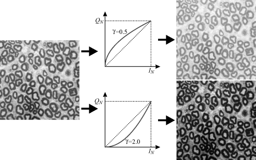
A common mapping is the gamma transformation. This is easier to represent when considering normalised values (where ![]() and
and ![]() represent fractions between zero and one).
represent fractions between zero and one).
(6.5) ![]()
The gamma curve was designed primarily to compensate for nonlinearities in the transfer function at various stages within the imaging system. For example, the relationship between the drive voltage of a cathode ray tube (CRT) and the output intensity is not linear, but is instead a power law. Therefore, a compensating gamma curve is required to make the contrast appear more natural on the display. (This is complicated by the fact that our eyes are not linearly sensitive to intensity either.)
The effects of the gamma transformation can be seen in Figure 6.8. When γ is less than one, the curve moves up, increasing the overall brightness of the image. From the slope of the curve, the contrast is increased for smaller pixel values at the expense of the lighter pixels, which have reduced contrast. For γ greater than one, the opposite occurs. The image becomes darker and the contrast is enhanced in the lighter regions at the expense of the darker regions.
Figure 6.8 The effects of a gamma transformation.
A sigmoid curve is also sometimes used to selectively enhance the contrast of the mid-tones at the expense of the highlights and shadows (Braun and Fairchild, 1999).
6.1.2 Global Thresholding and Contouring
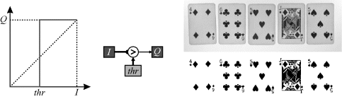
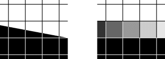
Thresholding, in its basic form, compares each pixel in the image with a threshold level and assigns the output to true or false (white or black) as shown in Figure 6.9. Since each pixel is treated identically, thresholding is a point operation.
Figure 6.9 Simple global thresholding.
Thresholding effectively classifies each pixel into one of two classes and is commonly used to segment between object and background. An appropriate threshold level can often be selected by analysing the statistics of the image, for example as contained in a histogram of pixel values. Several such threshold selection methods are described in Section 7.1.4 under histogram processing.
Sometimes, however, a single global threshold does not suit the whole image. Consider the example in Figure 6.10. The optimum threshold for one part of the image is not the optimum for other parts. Using a global threshold to process such images will involve a compromise in the quality of the thresholding of some region. A point operation is unsuitable to process such images, because to give good results over the whole image the operation needs to take into account not only the input pixel value but also the local context. Such images require adaptive thresholding, a form local filtering, and is considered further in Section 8.7.
Figure 6.10 Global thresholding is not always appropriate. Left: input image; centre: optimum threshold for the bottom of the image; right: optimum threshold for the top of the image.
Simple thresholding may be generalised to operate with more than one threshold level.
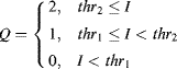
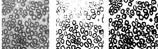
An example of this is shown in Figure 6.11. Here, two thresholds have been used to separate the image into three regions: the background, the cards and the pips. Each output pixel is assigned a label based on its relationship to the two threshold levels.
Figure 6.11 Multilevel thresholding.
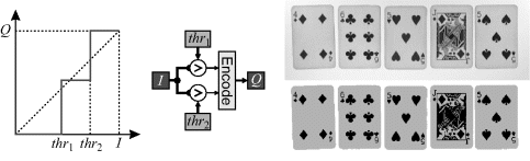
In this example, the darkest region is never adjacent to the lightest region. This it not the case in Figure 6.12, where the interior of the white bubbles is black. There is also a gradation in contrast between the white and black giving a ring of pixels within the bubbles detected as the intermediate background level. However, even if there was a sharp change in contrast between the black and white, many of the boundary pixels are still likely to have intermediate levels. This is because images are area sampled; the pixel value is proportional to the average light falling within the area of the pixel. Therefore, if the boundary falls within a pixel, as illustrated in Figure 6.13, part of the pixel will be white and part black, resulting in intermediate pixel values. Any blurring or lens defocus will exacerbate this effect.
Figure 6.12 Misclassification problem with multilevel thresholding. Left: original image; centre: classifying the three ranges; right: the background level labelled with white to show the misclassifications within each bubble.
Figure 6.13 Edge pixels have an intermediate pixel value.
Consequently, with multilevel thresholding, it is inevitable that some of the boundary pixels will fall between the thresholds and will be assigned an incorrect label. Such misclassifications require the information from the context (filtering) either as preprocessing before the thresholding, or after thresholding to reclassify the incorrect incorrectly labelled pixels.
Another form of multilevel thresholding is contouring. This selects pixel values within a range, as seen in Figure 6.14, and requires a minor modification to Equation 6.7:
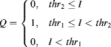
Figure 6.14 Contouring selects pixels within a range of pixel values.
Contouring is so named because, in an image with slowly varying pixel values, the pixels selected appear like contour lines on a map. However, contouring is less effective on high contrast edges, because it is detecting the intermediate pixel values illustrated in Figure 6.14. For a given threshold range, only a few edge pixels may fall within the range, and there is no guarantee that these pixels would be connected. While the pixels detected are likely to be edge pixels (depending on the threshold range), contouring makes a poor edge detector because it lacks the context required to give connectivity.
As the output after thresholding is binary, it only requires a single bit of storage per pixel. (More bits would be required for the output from multilevel thresholding, although this is usually significantly less than that of the input image.) Therefore, if an image is able to be successfully thresholded as it is streamed from the camera, the memory requirements for buffering the image are significantly reduced.
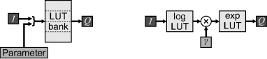
6.1.3 Lookup Table Implementation
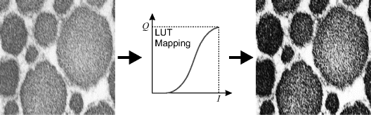
Most of the point operations considered so far are relatively simple mappings and can be implemented directly using logic. More complex mappings, such as gamma adjustment, require considerable logic to implement directly. If necessary, if such operations were implemented in logic, pipelining can be used to improve the speed.
Since the output value depends only on the input, the mapping for any point operation can be precalculated and stored in a lookup table. Then it is simply a case of using the input pixel value to index into the table to find the corresponding output. An example of this is shown in Figure 6.15.
Figure 6.15 Performing an arbitrary mapping using a lookup table.
The biggest advantage of a lookup table implementation is the constant access time, regardless of the complexity of the function. The size of the table depends on the width of the input stream, with each extra bit on the input doubling the size of the table.
A disadvantage of using a lookup table is that once the table has been set, the mapping is fixed. If the mapping is parameterised (for example contrast enhancement or thresholding) then it is also necessary to build logic to construct the lookup table before the frame is processed. Constructing the table will use the same (or similar) logic as implementing the point operation directly. The only difference is that timing is less critical. In a system with a software coprocessor, it may also be possible to construct the table in software rather than building hardware to calculate the table values.
If the parameter can be reduced to a small number of predefined values, then one alternative is to use the parameter to select between several preset lookup tables (as shown on the left in Figure 6.16). This is achieved by concatenating the parameter with the input pixel value to form the table address. Another possibility for more complex parameterised functions is to combine one or more lookup tables with logic, as shown for the gamma mapping on the right in Figure 6.16.
Figure 6.16 Parameterised lookup tables. Left: using the parameter as an address; right: combining tables with logic (implementing the gamma mapping).
A sequence of two or more point operations is in itself a point operation. For example, contrast enhancement followed by thresholding is equivalent to thresholding with a different threshold level. This property of point operations implies that a complex sequence of point operations may be replaced by a single lookup table that implements the whole sequence in a single clock cycle.
6.2 Point Operations on Multiple Images
Point operations can be applied not only to single images, but also between multiple images. For this, Equation 6.1 is extended to:
(6.9) ![]()
Corresponding pixels of the images are combined by an arbitrary function, ![]() , to give the output pixel value at the corresponding pixel location.
, to give the output pixel value at the corresponding pixel location.
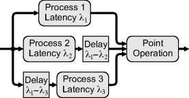
There are two main ways in which multi-image point operations are used. One is between two or more images derived from the same input image. A variation of this is between images derived from different, but synchronised, sensors. Stream processing requires that the streams for each of the images be synchronised. If the processing branches prior to the point operation have different latencies, then it will be necessary to introduce a delay within the faster branches to equalise the latency with the slowest branch. This is shown in Figure 6.17 for a three-input point operation. Note that the delay does not necessarily need to follow the faster process (as with Process 2); it may be inserted before it (as with Process 3), or even distributed throughout the process. However, keeping the delay together enables a more efficient implementation using shift registers or a FIFO buffer.
Figure 6.17 Two-image point operation applied to the same input image. A delay is inserted into the faster branch to equalise the latency.
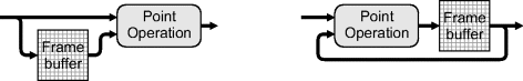
The other way is to apply the point operation between images captured at different times. This requires one or more frame buffers to hold the data from previous frames, as shown in Figure 6.18. Direct sequential access operates directly on the input image and one or more previous images. Recursive access feeds the output image back to be combined in some way with the incoming input image. In both cases, the frame buffer is used for both reading and writing. Some of the techniques of Section 5.2.1 may need to be used to enable the multiple parallel accesses.
Figure 6.18 Two-image point operation applied to successive images. Left: sequential access; right: recursive access. A frame buffer is required to hold the image from the previous frame.
Just as single image point operations may be implemented using a lookup table, lookup tables may also be used to implement multiple image point operations. The table input or address is formed by concatenating the individual inputs. The main limitation of this approach is that the memory requirement of a table grows exponentially with the number of address lines. This makes multiple input point operation lookup tables impractical for all but the most complex operations, or where the latency is critical. As with single input lookup tables, the latency of multiple input LUTs is constant at one clock cycle.
While there are potentially many multi-image point operations, this section focuses primarily on some of the more common ones.
6.2.1 Image Averaging
Real images inevitably contain noise, both from the imaging process and also from quantisation when creating a digital image. Let the captured image be the sum of the ideal, noise-free image and a noise image:
(6.10) ![]()
By definition, the noise-free image is the same from frame to frame. Let the noise have zero mean, and be independent from frame to frame:
(6.11) ![]()
where ![]() is the expectation operator. The signal-to-noise ratio (SNR) of the noisy image is then defined by the ratio of the energy in the signal to the energy in the noise. One definition of this is:
is the expectation operator. The signal-to-noise ratio (SNR) of the noisy image is then defined by the ratio of the energy in the signal to the energy in the noise. One definition of this is:
(6.12) ![]()
If several images of the same scene are averaged:
(6.13) ![]()
where:
(6.14) ![]()
then:
(6.15) 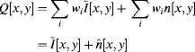
The image content is the same from frame to frame, so will reinforce when added. However, since the individual noise images are independent, the noise in one frame will partially cancel the noise in other frames. The noise variance will therefore decrease and is given by (Mitra, 1998):
If averaging a constant number of images, ![]() , the greatest noise reduction is given when the weights are all equal. The output signal-to-noise ratio is then:
, the greatest noise reduction is given when the weights are all equal. The output signal-to-noise ratio is then:
Note that the signal-to-noise ratio depends on the noise variance. The noise amplitude will therefore decrease by ![]() .
.
There is also a limitation with averaging multiple frames to reduce quantisation noise. If the noise from other sources (before quantisation) is significantly less than one pixel value, then the quantisation noise will be similar from one frame to the next. The noise term will no longer be independent and the reduction given by Equation 6.16 will no longer apply. On the other hand, if the noise standard deviation from other sources has a standard deviation larger than one pixel value, then the quantisation noise will be independent and will be reduced by averaging.
The main problem with averaging multiple frames is the requirement to store the previous ![]() frames in order to perform the averaging. Alternatively, this limitation may be overcome if the output frame rate is reduced by a factor of
frames in order to perform the averaging. Alternatively, this limitation may be overcome if the output frame rate is reduced by a factor of ![]() . In this latter case, the images are accumulated until
. In this latter case, the images are accumulated until ![]() have been summed, then the accumulator is reset to begin accumulation of the next
have been summed, then the accumulator is reset to begin accumulation of the next ![]() .
.
To overcome this limitation, one technique is to have an exponentially decreasing sequence of weights.
(6.18) ![]()
This may be implemented efficiently by calculating the result recursively:
The output noise variance, from Equation 6.16, is then given by:
(6.20) 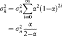
with the resulting signal-to-noise ratio:
By equating Equation 6.21 with Equation 6.17, the weight to give an equivalent noise smoothing to averaging ![]() images is:
images is:
The assumption with this analysis is that no additional noise is introduced by the averaging process. In practise, the result of multiplication by ![]() will require truncating the result. This will introduce additional noise, limiting the improvement in signal-to-noise ratio. To reduce this additional noise, it is necessary to maintain additional guard bits on the accumulator image.
will require truncating the result. This will introduce additional noise, limiting the improvement in signal-to-noise ratio. To reduce this additional noise, it is necessary to maintain additional guard bits on the accumulator image.
An example implementation of Equation 6.19 is shown in Figure 6.19. Since the frame buffer will almost certainly be off-chip memory, one of the schemes of Section 5.2.1 will need to be used to enable the accumulated image to be both read and written for each pixel. For practical reasons, ![]() can be made a power of two, enabling the multiplication to be implemented with a fixed binary shift. If
can be made a power of two, enabling the multiplication to be implemented with a fixed binary shift. If ![]() then the effective noise averaging window, from Equation 6.22, is:
then the effective noise averaging window, from Equation 6.22, is:
(6.23) ![]()
Figure 6.19 An implementation of weighted image averaging using Equation 6.19.
In most applications, this restriction is not a problem.
6.2.2 Image Subtraction
The main purpose for subtracting images is to determine the similarity between two images. Two global metrics are commonly used to gauge similarity: the sum of absolute differences (SAD):
and the sum of squared differences (SSD):
By squaring the difference, the ![]() effectively gives more weight to large differences.
effectively gives more weight to large differences.
One application of these metrics is in image registration. The spatial offset of one of the images is adjusted to obtain an estimate of the similarity as a function of position.
(6.26) ![]()
The offset corresponding to the minimum ![]() or
or ![]() is therefore the offset that makes the images most similar, and therefore provides an estimate of the relative position of the images to the nearest pixel. Image registration is discussed in more detail in Section 9.5.
is therefore the offset that makes the images most similar, and therefore provides an estimate of the relative position of the images to the nearest pixel. Image registration is discussed in more detail in Section 9.5.
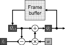
Another application of image subtraction is to detect changes within the scene. This is illustrated in Figure 6.20. Where there is no change, the difference between pixel values will be zero and any changes in the image will result in non-zero difference. This allows not only the addition or removal of objects to be detected, but also subtle shifts in the position of the object, which result in differences at intensity edges within the image.
Figure 6.20 Image subtraction to detect change. Left: original scene; centre: the changed scene; right: the difference image (offset to represent zero difference as a mid-grey).
Offsetting the pixel values so that no difference is represented by mid-grey enables both positive and negative differences to be represented. Any small shift in the image contents between the compared frames results in a bas relief effect, as seen in the difference image in Figure 6.20. Analysing the pixel values and thickness of these features enable even subpixel shifts to be detected.
Note that it is important when subtracting images taken at different times that the lighting remains constant or the images be normalised. This is particularly difficult with outdoor scenes, where there is little control over the lighting. There are two basic approaches to managing this problem. One is to take differences only between images closely spaced in time, where it is assumed that conditions do not change significantly from frame to frame, and the other is to maintain a dynamic estimate of the background that adapts as conditions change.
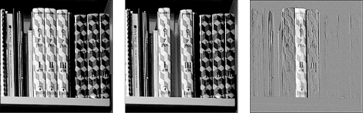
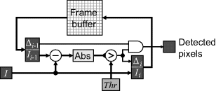
The principle behind frame differencing is that, when an object moves, part of the background in the previous image becomes obscured, resulting in a change in pixel value (assuming the object and background have different pixel values). One of the limitations of frame differencing is that there will also be a difference where the object was, as the background is uncovered. This is shown clearly in Figure 6.21. While in this case the previous position and current position can be distinguished by the sign of the difference, in general, with a complex background and objects this will not be the case. Significant differences are detected by thresholding the absolute difference. Double differencing (Kameda and Minoh, 1996) then detects regions that are common between successive difference images using a logical AND. It therefore detects objects that are arriving in the first difference and leaving in the second.
Figure 6.21 Double difference approach. Top: three successive input images; middle: differences between successive images; bottom, left and centre: absolute differences above the threshold; bottom, right: the double difference.
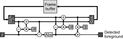
Although the double difference requires data from three frames, the recursive architecture introduced in Figure 6.19 can be readily adapted, as illustrated in Figure 6.22. The input pixel value is augmented with one extra bit (Δ) to indicate that the pixel has been detected as different between the last two frames. This difference bit is then combined with the difference bit stored with the previous frame to give the detected output pixels.
Figure 6.22 Implementing double differencing.
For more slowly moving objects (that obscure the background for several successive images) it is necessary that the object has sufficient texture to create differences in both difference frames. Double differencing has been applied to vehicle detection using an FPGA implementation (Cucchiara et al., 1999).
The alternative is to construct a model of the static background and take the difference between each successive image and the background. To account for changing conditions, it is necessary for the background image (or model) to be adaptive. Such background models can vary significantly in complexity (McIvor et al., 2001).
The simplest model is to represent the background image by the mean (Heikkila and Silven, 1999) or median (Cutler and Davis, 1998) of the previous several images. The median is less sensitive to outliers, but requires maintaining a large number of images to calculate. The mean, however, can be estimated using the recursive update of Equation 6.19. In this equation, ![]() controls how quickly changes to the scene are updated into the background. Larger values of
controls how quickly changes to the scene are updated into the background. Larger values of ![]() result in faster adaption of the background and rapid assimilation of objects into the background, but may result in artefacts of trails behind moving objects as they are partially assimilated into the background (Heikkila and Silven, 1999).
result in faster adaption of the background and rapid assimilation of objects into the background, but may result in artefacts of trails behind moving objects as they are partially assimilated into the background (Heikkila and Silven, 1999).
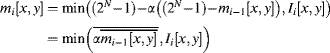
A problem with such a simple model is that it is unable to cope with regions of the image that are naturally variable, for example leaves fluttering in the wind. By estimating the variance associated with each pixel, pixels that vary significantly may be either masked out or only be detected as foreground object pixels if the difference exceeds three standard deviations (Orwell et al., 1999). Equation 6.19 may be adapted to efficiently derive an estimate of the variance:
Calculating the standard deviation requires taking the square root of the variance. A simpler alternative is to replace the standard deviation with the mean absolute deviation:
(6.28) ![]()
Again, the recursive architecture of Figure 6.19 can be extended to detect foreground pixels. Figure 6.23 replicates the mean update logic to calculate the mean absolute deviation. All pixels that differ from the mean by more than three deviations are detected as foreground pixels. As before, it is desirable to have ![]() to be a power of two to reduce the logic. The multiplication of the deviation by three can also be implemented with a shift and add.
to be a power of two to reduce the logic. The multiplication of the deviation by three can also be implemented with a shift and add.
Figure 6.23 Detecting foreground pixels using the mean and mean absolute deviation.
A limitation of the mean and variance approach is that the large variance (or mean absolute deviation) is often the result of two or more different distributions being represented by a pixel. For example, with a flag waving in the wind a pixel may alternate between the background and one of the colours on the flag. More sophisticated models account for the bimodal and multimodal pixel value distributions resulting from such effects. They represent each pixel by a weighted mixture of Gaussians (Stauffer and Grimson, 1999). To be effective, the mixture and Gaussian parameters need to be updated online as each image is acquired. The basic approach (Stauffer and Grimson, 1999) is to determine which of the Gaussians is represented by the current pixel (starting with the Gaussian that has the most weight). If it is within 2.5 standard deviations of the mean of one of the Gaussians, the pixel value is incorporated into that Gaussian, using Equations 6.19 and 6.27. The weights for all of the Gaussians in the mixture are updated using a similar weighted update, increasing the weight of the matched Gaussian and decreasing the weights of the others. If none of the Gaussians in the mixture matches the current pixel, the Gaussian with the least weight is discarded and replaced by a new Gaussian with a large standard deviation and low weight. The most probable Gaussians are considered background and the lowest weight Gaussians represent new events, so are considered to be foreground object pixels.
A significant advantage of the mixture model over a single Gaussian occurs when an object stops long enough to become part of the background, and then moves away again. The single Gaussian model will gradually drift to the new pixel value and then drift away again, resulting in an object being detected for a considerable time after it moves. With the mixture model, however, the mean does not drift, but a new distribution is begun for the object. When this receives sufficient weight, it is considered background. The model for the original background is retained, so when the object moves again, the pixels are correctly classified as background.
Typically, three to five Gaussians are used to model most images (McIvor et al., 2001). An FPGA implementation would be a relatively straightforward extension of Figure 6.23. Using more terms for each pixel requires more storage and logic to maintain the model. This may require multiple external RAM banks to give the required memory width. Alternatively, the frame rate can be reduced to enable sequential memory locations to be used for the component distributions. Appiah and Hunter (2005) have implemented a slightly simpler version of multimodal background modelling using a fixed width rather than explicitly modelling Gaussians. Their implementation considered both greyscale and colour images.
Other, more advanced and more complex methods of background estimation and subtraction have been reviewed by Piccardi (2004).
6.2.3 Image Comparison
Image addition and subtraction of successive images may be considered as a form of temporal filtering. Another type of filter useful for background estimation is to select the median (Cutler and Davis, 1998), maximum or minimum pixel value of successive images. The median is used in a similar manner to image averaging as described earlier. A problem with using the median, however, is that multiple images must be stored to enable its calculation on a pixel-by-pixel basis. The memory storage and consequent bandwidth issues restrict the usefulness of median calculation to short time windows for real-time operation.
If it is desired to detect dark objects moving against a light background, then the maximum of successive images may be able to estimate the background (Shilton and Bailey, 2006). Sufficient images must be combined so that for each pixel, at least one image within the set contains a background pixel. This may be implemented directly with the recursive architecture.
This makes using the maximum (or conversely using the minimum to estimate a dark background with light objects) practical. Only the maximum (or minimum) found so far needs to be stored.
Two limitations of Equation 6.29 are that any outlier will automatically become part of the background and, if conditions change, the background is unable to adapt. These may be overcome by building a decay into the expression:
where ![]() is slightly less than one. The multiplication may be replaced by a subtraction by choosing:
is slightly less than one. The multiplication may be replaced by a subtraction by choosing:
(6.31) ![]()
When working with the minimum, such a multiplication does not work as well. In this case, it is necessary to invert the image before scaling, so that the decay is toward white rather than black:
In practise, the inversion may be performed efficiently by taking the one's complement. Expressing Equation 6.32 in terms of its dual puts it in the same form as Equation 6.30:
(6.33) ![]()
The disadvantage of the multiplication is that the amount of the decay depends on the pixel value. An alternative is simply to subtract a constant:
(6.34) ![]()
where Δ is related to the expected noise level. The constant offset may also be used for estimating a dark background:
(6.35) ![]()
An implementation of this using the recursive architecture is shown in Figure 6.24.
Figure 6.24 Estimating a light background using a recursive maximum.
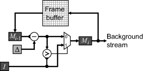
Image comparison is also used for adaptive thresholding. Instead of using a constant global threshold as in Equation 6.6, the threshold level is made to depend on the local context:
(6.36) ![]()
Equivalently, the comparison may be performed by subtracting the two images and then using a single global threshold.
Determining the threshold from the context requires some form of local filtering. Adaptive thresholding are therefore discussed in more detail in Section 8.7 in the context of filters.
6.2.4 Intensity Scaling
Multiplication or division can be used to selectively enhance the contrast within an image. One image is usually the input image being enhanced, and the other image represents the pixel dependent gain. As described earlier, a gain greater than one will increase the contrast and a gain less than one will reduce the contrast. The gain image is often obtained by preprocessing the input image in some way.
One application of pixel-by-pixel division is correcting for non-uniform pixel sensitivity within the image sensor, or vignetting caused by the lens. If the pixel response is nonlinear, then correction requires characterising the nonlinearity function, which is potentially different for each pixel (Sawchuk, 1977). Fortunately, most modern solid-state sensors are linear, enabling a simpler correction. The basic principle is to characterise the response by capturing an image of a uniform field. This approach is also able to correct for uneven illumination, provided the illumination is unchanged in the images being corrected.
Firstly, it is necessary to capture a reference image of a uniform field or a plain, non-textured background. Since the image should be uniform, any variation in pixel value is a result of deficiencies in the capture process, whether caused by variations in sensor gain or illumination. An image of a scene can then be corrected by dividing by the reference image (Aikens et al., 1989):
where the constant ![]() controls the dynamic range of the output image and is chosen so that the full range of pixel values is used. If the input and reference images are captured under identical conditions, then
controls the dynamic range of the output image and is chosen so that the full range of pixel values is used. If the input and reference images are captured under identical conditions, then ![]() is typically set to 255 (or
is typically set to 255 (or ![]() ). For practical implementation,
). For practical implementation, ![]() can be combined with the reference image to avoid the extra operation. After calibration, the reference image does not change. Therefore, the processing complexity of Equation 6.37 may be reduced by converting the division to a multiplication and precalculating
can be combined with the reference image to avoid the extra operation. After calibration, the reference image does not change. Therefore, the processing complexity of Equation 6.37 may be reduced by converting the division to a multiplication and precalculating ![]() .
.
For best accuracy, when capturing the reference image the exposure should be as large as possible without actually causing any pixels to saturate. In practise, a uniform illumination field is difficult to achieve (Schoonees and Palmer, 2009) but a similar reference image may be obtained by processing a sequence of images of a moving background containing a modulation pattern. The processing enables the variations caused by the imaging process to be separated from the variations in the illumination (Schoonees and Palmer, 2009).
Note that any errors or noise present in the reference image will be introduced into the image through Equation 6.37. It is therefore important to minimise the noise. This may be accomplished, if necessary, by averaging several images or applying an appropriate noise smoothing filter.
Once calibrated, the reference image needs to be stored so that it can be made available as needed for processing. The large size of an image requires an external memory to use as a frame buffer in most circumstances. However, as the reference image is generally slowly varying, it can be compressed readily. A simple compression scheme would be to down-sample the reference image and reconstruct the reference using interpolation. Down-sampling by a factor of 8 or 16 would give a significant data reduction, enabling the reference to be stored directly on the FPGA. See Section 9.3 for an implementation of the reference reconstruction process.
When considering only vignetting, an alternative approach is to model the intensity fall off with radius (Goldman and Chen, 2005). The model can then be used to perform the correction, rather than requiring a reference image.
Other applications of normalisation include colour balancing and colour space conversion. For example, calculating the colour saturation requires normalising by the intensity. This, and other related colour transformations are described in more detail in Section 6.3.
Correlation is another image operation that requires multiplication of images on a pixel-by-pixel basis. The resulting product is then summed over the image:
(6.38) ![]()
Like the sum of squares or absolute differences, this is a measure of the similarity of two images, with a larger correlation indicating a better match. Like the sum of differences, correlation is also used for image registration, by adjusting the offset of one of the images to maximise the correlation. It can be shown that correlation is closely related to the minimum square difference (Jain, 1989). Expanding Equation 6.25 gives:
(6.39) 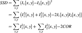
The first two terms are constant when registering images, so maximising the correlation is equivalent to minimising the sum of squared difference.
The problem with simple correlation for image registration is that images are finite. Therefore, if the image is darker on one side than the other, this can introduce a bias that offsets the correlation peak. This may be overcome by normalising the correlation by the overlap area and average pixel value (Jain, 1989):

This requires maintaining three accumulators for each correlation output: one for ![]() , one for
, one for ![]() and one for
and one for ![]() . The division and square root are only performed at the end of the image, rather than at every pixel, so their speed is much less critical.
. The division and square root are only performed at the end of the image, rather than at every pixel, so their speed is much less critical.
6.2.5 Masking
The final operation that will be considered in this Section is image masking. In its most basic form it consists of a logical AND or OR operation. Masking is commonly used to select a region of an image to process, while ignoring irrelevant regions within the image. The choice to use an AND or OR depends on the desired level for the background. ANDing with zero will result in a black background, while ORing with one will make the background white. These options are shown schematically in Figure 6.25.
Figure 6.25 Masking, with setting of the background to black or white.
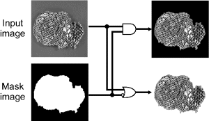
Logical OR and AND can also be used to combine multiple regions into a single image. OR is used with a black background and AND with a white background. The result is a generalisation of multiplexing, using a set of mask images to select the corresponding image data for the output.
One application of this is image compositing, creating a single image from a series of offset images, for example when making a panorama from a series of panned images. To ensure a good result, it is necessary to correct for lens and other distortions and to ensure accurate registration in the region of overlap. Where the scene geometry is known, this may be accomplished by rectifying the images (Bailey and Shand, 1996). If the images are subject to vignetting, the seams between the images can be visible. Correcting for vignetting (Goldman and Chen, 2005) can significantly improve the results by making the pixel values of on each side of the join similar.
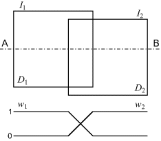
Rather than switch from one image to the other at the border between the images, the seam resulting from mismatched pixel values between the images may be significantly reduced by merging the images in the region of the overlap. Consider two overlapping frames, ![]() and
and ![]() , as illustrated in Figure 6.26. In the region of overlap the two frames are merged with a smooth transition from one to the other. The weights applied to each of the images,
, as illustrated in Figure 6.26. In the region of overlap the two frames are merged with a smooth transition from one to the other. The weights applied to each of the images, ![]() and
and ![]() respectively, depend on the width of overlap, which may vary from image to image, and also with position within the image.
respectively, depend on the width of overlap, which may vary from image to image, and also with position within the image.
Figure 6.26 Merging of images in the overlap region. The weights corresponding to the input images are shown for the Section A–B.
One relatively simple technique is to apply the distance transform to each of the mask images. This labels each pixel within the mask image with the distance to the nearest edge of the mask (distance transforms are covered later in Section 11.5). The weights may then be calculated from the distance transformed masks, ![]() and
and ![]() :
:
(6.41) ![]()
The output image is then given by:
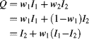
An implementation of Equation 6.42 suitable for streamed operation is shown in Figure 6.27. Note that these operations are applied for each pixel within the image. The rearrangement in Equation 6.42 reduces the computation to a single division to calculate the weight and a single multiplication to combine the two images. The calculation may require pipelining to meet timing constraints.
Figure 6.27 Schematic for merging images, given distance weighted masks.
Colour image processing is a logical extension to the processing of greyscale images. The main difference is that each pixel consists of a vector of components rather than a scalar. A vector-based image can be defined as ![]() , where:
, where:
(6.43) ![]()
or
(6.44) 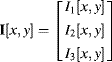
and ![]() ,
, ![]() ,
, ![]() are the component images. If the colour image is split into its component parts, then a point operation on a colour image can be considered to be a point operation on multiple images.
are the component images. If the colour image is split into its component parts, then a point operation on a colour image can be considered to be a point operation on multiple images.
The most common native representation of an image is for each pixel to have red, green and blue components, ![]() , corresponding approximately with the sensitivity of the cones within the human visual system. As described in Section 1.2, a colour image is usually formed by capturing images with sensors that are selectively sensitive to the red, green and blue regions of the spectrum. Colour is typically represented by a three-dimensional vector, and the most common standard is to have eight bits per component, resulting in a 24-bit colour system.
, corresponding approximately with the sensitivity of the cones within the human visual system. As described in Section 1.2, a colour image is usually formed by capturing images with sensors that are selectively sensitive to the red, green and blue regions of the spectrum. Colour is typically represented by a three-dimensional vector, and the most common standard is to have eight bits per component, resulting in a 24-bit colour system.
Sensors are not solely restricted to the visible region of the electromagnetic spectrum. Each spectral band conveys different information about the properties of the object being imaged. Such multispectral imaging, particularly in the infrared, has been found useful in a wide range of applications, including land use and vegetation classification in remote sensing (Ehlers, 1991) and produce grading (Duncan and Leeson, 1999) for detecting blemishes that may not be as apparent in the visible spectrum.
Colour image processing, therefore, involves the processing of such vector-valued images.
6.3.1 False Colouring
The first operation considered is false colouring. This is so named because the colours seen in the output image are false in that they do not reflect the true underlying colour of the scene. The purpose of false colouring is to make apparent to a human viewer that which may not be apparent or visible in the original image. It is seldom used as part of an automatic image processing algorithm.
False colouring is applied in two distinct ways. The first is to map the non-visible components of a multispectral image into the visible region of the spectrum. This enables human viewing (and interpretation) of the resultant image. For example, in remote sensing, different types of vegetation have different spectral signatures that are most obvious in the near infrared, red and green components (Duncan and Leeson, 1999). Therefore, a mapping commonly used within remote sensing is to map these onto the red, green and blue components respectively of the output image or display. The resulting colours are not the same as seen by the unaided human eye. However, they do allow subtle distinctions to be more readily seen and distinguished.
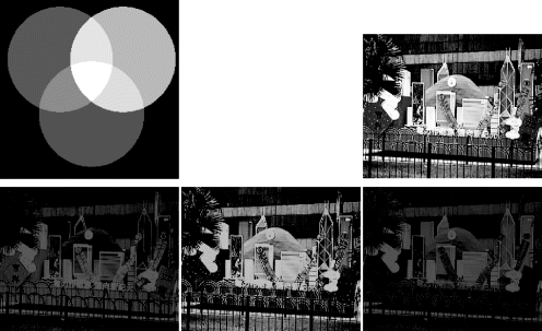
A related technique is to combine different images of the same scene as the different components of a colour image. One example where this has been used is to verify the correct registration of images taken from different viewpoints (Reulke et al., 2008). The images from each viewpoint are registered to a common coordinate system, and when combined, they should align. Any registration errors will show as coloured fringes. A similar application is to combine images taken at different times as different components, as shown in Figure 6.28. Common regions within the set will show up as grey because they have equal red, green and blue components. However, any differences will cause an imbalance in the components, resulting in a coloured output. In the example here (Figure 6.28), dark objects appear in their complimentary colour: the dark second hand in the red channel appears cyan, dark in the green channel appears magenta, and dark in the blue channel appears yellow.
Figure 6.28 Temporal false colouring. Images taken at different times are assigned to different channels, with the resultant output showing coloured regions where there are temporal differences. (See colour version of this figure in colour plate Section)
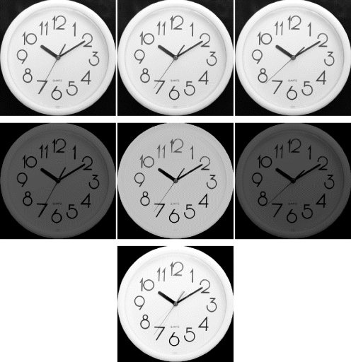
The second way in which false colouring is commonly used is to map a greyscale image onto a colour image. Each pixel value is assigned a separate colour. This is implemented by using a lookup table to produce each of the red, green and blue components, as shown in Figure 6.29. Its usefulness relies on the ability of the human visual system to more readily distinguish colours than shades of grey, particularly when the local contrast is different (see, for example, Figure 6.3). An appropriate pseudocolour both enhances the contrast, and can facilitate the manual selection of an appropriate threshold level.
Figure 6.29 Pseudocolour or false colour mapping using lookup tables. (See colour version of this figure in colour plate Section)
6.3.2 Colour Space Conversion
While the RGB colour space is native to most display devices, it is not necessarily the most natural to work in. Colour space conversion involves transforming one vector representation into another that makes subsequent analysis or processing easier. Colour space conversion is a point operation, since each pixel is operated on independently.
6.3.2.1 RGB
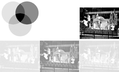
The RGB colour space is referred to as additive, because a colour is made by adding particular levels of red, green and blue light. Figure 6.30 illustrates this with the RGB components of a colour image.
Figure 6.30 RGB colour space. Top left: combining red, green and blue primary colours; bottom: the red, green and blue components of the colour image on the top right. (See colour version of this figure in colour plate Section)
The RGB colour components (whether from capture or display) are device dependent. In a scene captured by a camera, the colour vector for each pixel depends not only on the colour in the scene and the illumination, but also on the spectral response of the filters used to measure the red, green and blue components. Similarly, the actual colour produced on a display will depend on the spectral content of the red, green and blue light sources within the display. Therefore, there are many different RGB colour spaces depending on the particular wavelengths (or spectral mix) used for each of the red, green and blue primaries.
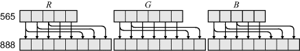
Two variations of RGB are of particular note. The first is 16-bit RGB. This is used where the entire colour vector must be contained within 16 bits, usually as a result of bandwidth limitations. With 16-bit RGB, five bits are allocated for each of the ![]() and
and ![]() components, and six bits are allocated for
components, and six bits are allocated for ![]() (to take into account the increased sensitivity of the human visual system to green). To convert from 16-bit to 24-bit RGB, rather than append zeros, it is better to append the two (for
(to take into account the increased sensitivity of the human visual system to green). To convert from 16-bit to 24-bit RGB, rather than append zeros, it is better to append the two (for ![]() ) or three (for
) or three (for ![]() and
and ![]() ) most significant bits of the component as shown in Figure 6.31.
) most significant bits of the component as shown in Figure 6.31.
Figure 6.31 Converting from RGB565 to RGB888.
The main limitation of the RGB colour space is that it is device dependent. To combat this, a device independent colour space was defined: sRGB (Stokes et al., 1996). This is a defacto standard for consumer colour devices, including cameras, printers and displays. It not only defines the specific colours of the three primaries used for red, green and blue, but also defines a nonlinear gamma-like mapping between the intensity and the numerical values that closely approximates the response of CRT-based displays.
Conversion from a device-dependent RGB to sRGB requires first multiplying the device dependent colour vector by a 3 × 3 matrix that depends on the red, green and blue spectral characteristics of the device. This transformation, determined by calibration, is sometimes called the colour profile of the device. The result of the transformation represents a vector of normalised (between zero and one) linear RGB values. Any component that is outside this range is outside the gamut of colours that may be reproduced within sRGB and is clipped to fall within this range. Each component, ![]() , is then mapped from linear RGB to sRGB values by (Stokes et al., 1996):
, is then mapped from linear RGB to sRGB values by (Stokes et al., 1996):
The final values can then be represented as 8-bit quantities by scaling by 255.
Equation 6.45 can be easily inverted to remove the gamma component and return to linear components:
(6.46) 
6.3.2.2 CMY and CMYK
In printing, rather than actively producing light, the image begins with the white paper, and colour is produced by filtering or blocking some of the colour. The subtractive primaries are cyan, magenta and yellow, and usually consist of appropriate inks, dyes or filters. Consider the yellow dye; it will allow the red and green spectral components to pass through, but will attenuate the blue, making that part of the scene appear yellow. The more yellow, the more the blue is attenuated, the yellower the scene will appear. Similarly, the magenta dye attenuates the green spectral component, and the cyan dye attenuates the red component. A CMY image is therefore formed from the cyan, magenta and yellow components:
![]()
Therefore, as illustrated in Figure 6.32, the colours of a scene may be produced by mixing different quantities of yellow, magenta and cyan dyes to give the required spectral content at each point. If the RGB components are normalised then the corresponding normalised CMY components are approximately given by:
Figure 6.32 CMY colour space. Top left: combining yellow, magenta and cyan secondary colours; bottom: the yellow, magenta and cyan components of the colour image on the top right. (See colour version of this figure in colour plate Section)

The exact relationship depends on the spectral content of the RGB components and the spectral transmissivity of the CMY components. While the simple conversion of Equation 6.47 works reasonably well with lighter, unsaturated colours, it becomes less accurate for darker and more saturated colours where one (or more) of the CMY components is larger. There are two reasons for this. Firstly, the attenuation is not linear with the amount of dye used, but is exponential. This makes the relationship approximately linear for lower levels of CMY components, but deviates more for the higher levels. Consequently, a particular spectral component cannot be completely removed, making it difficult to produce fully saturated colours and dark colours. The second reason is that equal levels of yellow, magenta and cyan seldom result in a flat spectral response. Both of these factors make black appear as a muddy colour often with a colour cast.
In printing, this problem is overcome with the addition of a black dye, resulting in the CMYK colour space. Equal amounts of yellow, magenta and cyan dyes are replaced by the appropriate amount of black dye. This changes the approximate conversion from Equation 6.47 to:
(6.48) 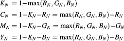
Note that one of the CMYK components will always be zero. Other than for printing, the CMY or CMYK colours spaces are not often used for image processing.
6.3.2.3 YUV, YIQ and YCbCr
When colour television was introduced, backward compatibility with existing black and white television was desired. The luminance signal, ![]() , is a combination of RGB components, with the colour provided by two colour difference signals,
, is a combination of RGB components, with the colour provided by two colour difference signals, ![]() and
and ![]() . Assuming normalised RGB, the image can be represented in YUV colour space,
. Assuming normalised RGB, the image can be represented in YUV colour space, ![]() , with the components given by:
, with the components given by:
The particular weights given for the ![]() component reflect the relative sensitivities of the human visual system. Representing Equation 6.49 in matrix form gives:
component reflect the relative sensitivities of the human visual system. Representing Equation 6.49 in matrix form gives:
The range of the ![]() component is from −0.615 to 0.615, which requires an extra bit to represent. When processing digitally, it is more common to adjust the scale factors of the
component is from −0.615 to 0.615, which requires an extra bit to represent. When processing digitally, it is more common to adjust the scale factors of the ![]() and
and ![]() components so both are in the range −0.5 to 0.5 (for example as used by the JPEG2000 standard (ISO, 2000)). This makes the transform matrix:
components so both are in the range −0.5 to 0.5 (for example as used by the JPEG2000 standard (ISO, 2000)). This makes the transform matrix:
(6.51) 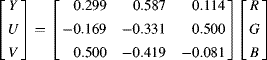
The YIQ colour space is very similar to the YUV, except for different weights in Equation 6.50:
(6.52) 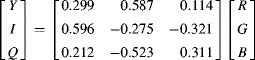
The difference is that the chrominance components ![]() are rotated by 33 degrees. This requires a full matrix multiplication (nine multiplications) rather than the five of Equation 6.49. The advantage gained is a reduction in bandwidth required for television broadcasting because the human visual system is less sensitive to the
are rotated by 33 degrees. This requires a full matrix multiplication (nine multiplications) rather than the five of Equation 6.49. The advantage gained is a reduction in bandwidth required for television broadcasting because the human visual system is less sensitive to the ![]() component than to the
component than to the ![]() component. The YIQ colour space, however, is seldom used for digital image processing.
component. The YIQ colour space, however, is seldom used for digital image processing.
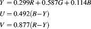
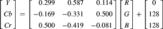
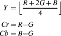
Strictly speaking, the YUV colour space is an analogue representation. The corresponding digital representation is called YCbCr, with ![]() . There are two commonly used YCbCr formats: one scales the values by less than 255 to give 8-bit quantities with headroom and footroom and offsets the chrominance components to enable an unsigned representation:
. There are two commonly used YCbCr formats: one scales the values by less than 255 to give 8-bit quantities with headroom and footroom and offsets the chrominance components to enable an unsigned representation:
(6.53) 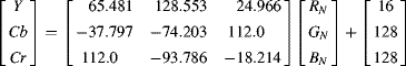
and the other uses the full range of 8-bit outputs for each of the components. This latter case is often used with 8-bit input images (from 0–255) where the headroom and footroom are not considered as important as maximising the dynamic range:
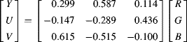
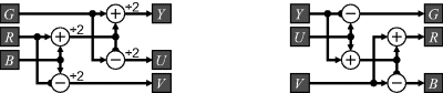
The implementation of Equation 6.54 will be considered here. This matrix can be factorised to use four multiplications:
(6.55) 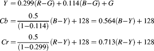
with the implementation shown in Figure 6.33. The inverse similarly requires four non-trivial multiplications.
(6.56) 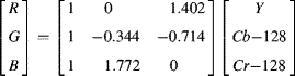
Figure 6.33 Left: conversion from RGB to YCbCr; right: conversion from YCbCr to RGB.
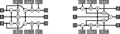
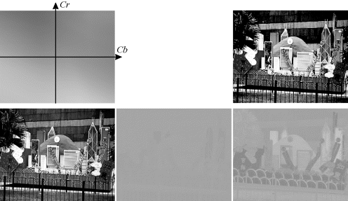
Since the multiplications are by constants, they may be implemented efficiently using a few additions. The addition and subtraction of 128 can be accomplished by just inverting the most significant bit. The YCbCr components of a colour image are illustrated in Figure 6.34.
Figure 6.34 YCbCr colour space. Top left: the ![]() colour plane at mid luminance; bottom: the luminance and chrominance components of the colour image on the top right. (See colour version of this figure in colour plate Section)
colour plane at mid luminance; bottom: the luminance and chrominance components of the colour image on the top right. (See colour version of this figure in colour plate Section)
From an image processing perspective, the advantage of using YUV or YCbCr over RGB is the reduction in correlation between the channels. This is particularly useful with colour thresholding as described in the next Section. It also simplifies the enhancement of colour images. For example, contrast enhancement (such as histogram equalisation) may be performed on the ![]() component of the image.
component of the image.
There are two limitations of the YUV (or YCbCr colour space). The first is that the transformation is a (distorted) rotation of the RGB coordinates. The scale factors are chosen to ensure that every RGB combination has a legal YCbCr representation; however, the converse is not true. Some combinations of YCbCr fall outside the legal range of RGB values. The implication is that more bits must be kept in the YCbCr representation if the transform is to be reversed. Note that this cannot be avoided when using rotation based transformation of the colour space.
The second limitation is that it requires either floating-point or fixed-point multiplications to perform the transformation. This problem is primarily caused by the different weights for the ![]() component, which are based on human perception of the luminance. From an image processing point of view, this is often less relevant and can be relaxed.
component, which are based on human perception of the luminance. From an image processing point of view, this is often less relevant and can be relaxed.
The obvious solution to this problem is to restrict the coefficients to powers of two. There are several ways of accomplishing this. One is the reversible colour transform (RCT) used by lossless coding in JPEG2000 (ISO, 2000). This has:
where ![]() represents truncation. Although information appears to be lost by the truncation, it is retained in the other two terms and can be recovered exactly (hence reversible colour transform). The
represents truncation. Although information appears to be lost by the truncation, it is retained in the other two terms and can be recovered exactly (hence reversible colour transform). The ![]() and
and ![]() terms would appear to require an extra bit to prevent wrap around, and this is mandated in the JPEG2000 standard, but this is actually unnecessary, since the
terms would appear to require an extra bit to prevent wrap around, and this is mandated in the JPEG2000 standard, but this is actually unnecessary, since the ![]() term provides sufficient information to resolve the ambiguity. The reverse transformation is:
term provides sufficient information to resolve the ambiguity. The reverse transformation is:
(6.58) 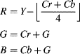
While this solution is good from a coding perspective, for many image processing algorithms the ambiguity between positive and negative values of ![]() and
and ![]() would need to be resolved by retaining the extra bit.
would need to be resolved by retaining the extra bit.
The RCT is not orthogonal; in particular, there is a strong correlation caused by the significant sharing of the ![]() component. One YUV-like orthogonal transformation is (Sen Gupta et al., 2004; Sen Gupta and Bailey, 2008):
component. One YUV-like orthogonal transformation is (Sen Gupta et al., 2004; Sen Gupta and Bailey, 2008):
A similar transformation is:
(6.60) 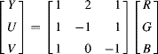
The problem with these is that the inverse transformations require division by three. An orthogonal transformation that uses powers of two for both the forward and inverse transformations is not possible. A minor adjustment to Equations 6.59 and gives a simple transform that is nearly orthogonal and is also easily inverted. Here it is represented in normalised form:
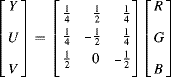
This may be further factorised to reduce the complete transformation to four additions, with the ÷2 performed by a shift, which is free in hardware. The implementation of this, and its inverse:
(6.62) 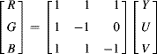
are shown in Figure 6.35.
Figure 6.35 A multiplier-less YUV-like transformation and its inverse.
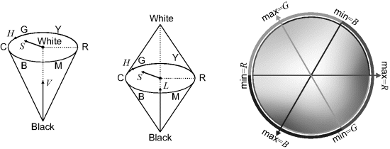
6.3.2.4 HSV and HLS
The RGB or YUV colour spaces do not reflect the psychological way in which colour is interpreted or thought about. When a colour is interpreted, it is considered primarily in terms of its hue and the strength of the colour (saturation) rather than the individual RGB components. Therefore, it is reasonable to have a colour space with hue, saturation and intensity as the three components. Two such colour spaces are ![]() (hue, saturation and value) and
(hue, saturation and value) and ![]() (hue, lightness, and saturation) (Foley and Van Dam, 1982).
(hue, lightness, and saturation) (Foley and Van Dam, 1982).
The HSV colour space is typically represented as a cone as shown in the left panel of Figure 6.36. The hue represents the angle around the cone, resulting in the colour wheel on the right panel of Figure 6.36. By definition, the black-white axis up the centre of the cone has a hue of zero. The remainder of the colour wheel is split into three sectors based on which component is the maximum, and the proportion between the other two components is used to give the angle. This is illustrated graphically in the colour wheel in Figure 6.36.
Figure 6.36 HSV and HLS colour spaces. Left: the HSV cone; centre: the HLS bi-cone; right: the hue colour wheel. (See colour version of this figure in colour plate Section)
Mathematically, the hue is defined as:
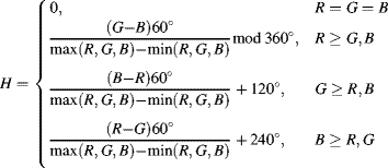
With a binary number system, the use of degrees (or even radians) is inconvenient. There are two alternatives. One is to normalise the angle so that a complete cycle goes from zero to one, which maximises the hue resolution for a given number of bits and avoids the need to manage wraparound of values outside the range of 0–360°. This may be preferable when performing many manipulations on the hue. The other is to represent 60° by a power of two (for example 64) to simplify the multiplication. It also makes it easier to convert back to RGB.
The value is similar to ![]() , except that equal weight is given to the red, green and blue components, rather than weighting them based on human perception. The
, except that equal weight is given to the red, green and blue components, rather than weighting them based on human perception. The ![]() component represents the height up the cone. The value is usually represented normalised between zero and one.
component represents the height up the cone. The value is usually represented normalised between zero and one.
(6.64) ![]()
The saturation represents the strength of the colour and is represented by the radius of the cone relative to the maximum radius for a given value:
(6.65) 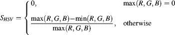
This normalisation means only the value changes as the intensity of the image is scaled. The HSV components of a sample image are shown in the middle row of Figure 6.37. Note that for greys in the input image the hue is meaningless, because even a small amount of noise on the components will determine the hue.
Figure 6.37 HSV and HLS colour spaces. Top left: HSV hue colour wheel, with saturation increasing with radius; middle row: the HSV hue, saturation and value components of the colour image on the top right; bottom row: the HLS hue, saturation and lightness components. (See colour version of this figure in colour plate Section)

The HLS representation is slightly different from the HSV colour space in that it is a bi-cone rather than a cone, as seen in the centre panel of Figure 6.36. The main advantage of HLS over HSV is that it is symmetric with respect to black and white. The hue is the same for both representations, given by Equation 6.63, but the lightness and saturation differ from the HSV space. Again, the lightness and saturation are usually represented as normalised values.
(6.67) 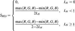
The HLS components of the sample image are shown in the bottom row of Figure 6.37.
Equation 6.66 places fully saturated primary colours at half lightness, at the interSection of the two cones. In general, this makes ![]() less than
less than ![]() , although this has no real consequence from an image processing perspective.
, although this has no real consequence from an image processing perspective.
The major limitation of HLS is that the saturation is only constant with scaling lightness only in the lower cone (![]() ). This gives the anomaly that pastel colours can appear as fully saturated. In particular, this can be seen in the lighter areas of Figure 6.37, where the saturation is high.
). This gives the anomaly that pastel colours can appear as fully saturated. In particular, this can be seen in the lighter areas of Figure 6.37, where the saturation is high.
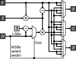
For these reasons, only the implementation of HSV will be considered here. Figure 6.38 shows an implementation of the conversion from RGB to HSV. The minimum and maximum components are determined from the sign bits of the differences between the input colour channels. These differences need to be calculated anyway to give the numerators of Equation 6.63, so this information is effectively obtained for free. Apart from the multiplexers to select the minimum and maximum components, the main complexity is the two dividers for normalising the hue and the saturation. The colour wheel is rotated so that a hue of zero corresponds to magenta to save the modulo normalisation when the maximum pixel is red. To achieve this, the offset added to the hue is given by:
Figure 6.38 Conversion from RGB to HSV.
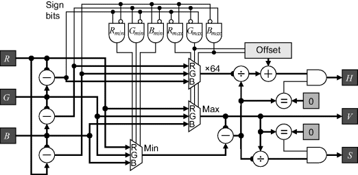
(6.68) ![]()
with the hue taking a value between zero and 383. If necessary, this can be shifted back by subtracting 64, and then adding 384 if the result goes negative.
To convert HSV back to RGB, the three most significant bits of the hue represent the sector, hence can be used to select the appropriate values for the RGB components:
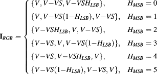
where the least significant bits of hue are considered as a fraction. An implementation of Equation 6.69 is shown in Figure 6.39.
Figure 6.39 Conversion from HSV to RGB.
A form of hue and saturation may also be derived from the YCbCr colour space by converting the chrominance components into polar coordinates (Punchihewa et al., 2005). This may be readily implemented using a CORDIC transformation.
(6.70) ![]()
(6.71) ![]()
In this form, the saturation will scale with intensity, which is generally not desired. To make the saturation more meaningful, it is necessary to scale the saturation by either the ![]() or the maximum RGB component so that it is not intensity dependent.
or the maximum RGB component so that it is not intensity dependent.
The HSV colour space is useful in image processing for colour detection and enhancement. The advantage gained is the intensity independence of hue and saturation, enabling more robust segmentation. One limitation, however, is the need to have a correct colour balance. The hue (and also the saturation to a lesser degree) is affected by any colour cast, especially for colours with low saturation. Section 6.3.4 considers correcting the colour balance of an image.
In some applications, only one part of the colour wheel is of interest. For example, many fruits vary in colour from green to yellow or red. In this case the sectors between green and red are of particular interest, whereas outside this range it less important. In these cases, a simplified substitute for hue may be used. For example, when analysing the colour of limes, colours in the range from green (chlorophyll dominates) to yellow (carotenoids dominate) are important (Bunnik et al., 2006); these may be captured by a ratio of the components:
This measure ranges from zero for pure green to one for yellow, enabling the health of the fruit to be assessed. Such a measure is less suitable for reds (such as would be encountered when grading tomatoes, where the red pigmented lycopene dominates), because the red component can be much larger than the green. A small change in the green component can result in a large change in the measure. An alternative hue measure that is more uniform is (Bunnik et al., 2006):
(6.73) ![]()
which ranges from −1 for pure greens through 0 for yellow to +1 for pure reds. Note that, as with the hue, both the measures of Equations 6.72 and require the correct scaling or balance between the red and green channels to accurately reflect the colour.
In other applications, other colour distinctions may be important, enabling similar simplifications to be used.
6.3.2.5 CIE XYZ and xyY
The limitation, as mentioned before, of RGB is that it is device dependent. In 1931, the International Commission on Illumination (CIE) established the XYZ standard colour space. The ![]() ,
, ![]() and
and ![]() are imaginary (in the sense that they do not correspond to any real illumination) tristimulus values chosen such that the
are imaginary (in the sense that they do not correspond to any real illumination) tristimulus values chosen such that the ![]() corresponds with perceived intensity, and all possible visible colours are represented by a combination of positive values of XYZ (Hoffmann, 2000). (It is impossible to produce all visible colours with only three real sources.)
corresponds with perceived intensity, and all possible visible colours are represented by a combination of positive values of XYZ (Hoffmann, 2000). (It is impossible to produce all visible colours with only three real sources.)
One limitation of a three-dimensional colour space is that it is difficult to represent graphically in two dimensions. Since the underlying colour does not change with changing intensity, a normalised colour space ![]() may be derived:
may be derived:
which then allows the colour or chromaticity to be represented by two of the components.
The ![]() plane is usually used to define the colour, resulting in the chromaticity diagram of Figure 6.40. Given two points on the chromaticity diagram corresponding to two colour sources, a linear combination of those sources will lie on a straight line between those points. Therefore, any three points, corresponding for example to red, green and blue light sources, can be mixed to produce only the colours within the triangle defined by those three points. To go outside the triangle would require one (or more) of the sources to have a negative intensity, which is clearly impossible. The triangle, therefore, defines the gamut of colours that can be produced by those primaries, for example on a display.
plane is usually used to define the colour, resulting in the chromaticity diagram of Figure 6.40. Given two points on the chromaticity diagram corresponding to two colour sources, a linear combination of those sources will lie on a straight line between those points. Therefore, any three points, corresponding for example to red, green and blue light sources, can be mixed to produce only the colours within the triangle defined by those three points. To go outside the triangle would require one (or more) of the sources to have a negative intensity, which is clearly impossible. The triangle, therefore, defines the gamut of colours that can be produced by those primaries, for example on a display.
Figure 6.40 Chromaticity diagram. The numbers are wavelengths of monochromatic light in nanometres. (See colour version of this figure in colour plate Section)

To convert from a chromaticity back to XYZ tristimulus values, it is also necessary to know the intensity, ![]() , resulting in the xyY representation. The
, resulting in the xyY representation. The ![]() and
and ![]() values may be recovered from
values may be recovered from
(6.75) 
With any linear tristimulus colour space, the component values may be transformed into any other linear colour space simply by a matrix multiplication (Hoffmann, 2000). The matrix used depends, of course, on the spectral characteristics of the particular components used. For example, the primaries used in HDTV have the chromaticity values listed in Table 6.1. The white point defines the chromaticity coordinates of white, defined as the colour observed when all three RGB components are equal.
Table 6.1 Chromaticity values for HDTV and sRGB.
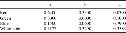
The corresponding transformation matrix and its inverse can then be derived as (Hoffmann, 2000):
(6.76) 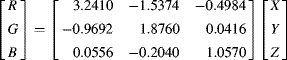
(6.77) 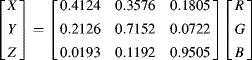
If device independence is not a requirement, a device-dependent chromaticity may also be formed. This normalises the RGB components in a similar manner to Equation 6.74:
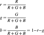
with the device dependent ![]() chromaticity shown in Figure 6.41.
chromaticity shown in Figure 6.41.
Figure 6.41 Device dependent ![]() chromaticity. (See colour version of this figure in colour plate Section)
chromaticity. (See colour version of this figure in colour plate Section)
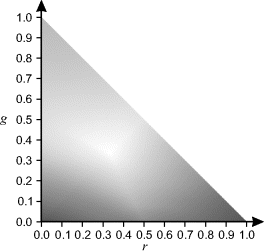
6.3.2.6 CIE L∗a∗b∗ and CIE L∗u∗v∗
One limitation of the colour spaces mentioned so far is that they are not perceptually uniform. In estimating colour differences or colour errors, it is useful if the distance between two points is a measure of the perceived colour difference. Several colour spaces have been derived from the CIE XYZ space that are perceptually more uniform. Two considered here are the CIE L∗a∗b∗ and CIE L∗u∗v∗ colour spaces.
The L∗a∗b∗ space is defined relative to a reference white point ![]() and introduces the following nonlinearity to make the space more uniform:
and introduces the following nonlinearity to make the space more uniform:
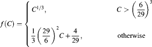
The conversion is to ![]() is then:
is then:
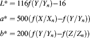
resulting in the lightness, ![]() , ranging from 0 to 100. A different range may be arranged by appropriate scaling. The
, ranging from 0 to 100. A different range may be arranged by appropriate scaling. The ![]() axis goes from green (negative) to red or magenta (positive), and the
axis goes from green (negative) to red or magenta (positive), and the ![]() axis goes from blue (negative) to yellow (positive).
axis goes from blue (negative) to yellow (positive).
The function, ![]() , may be implemented using a lookup table, although three will be required to convert one pixel per clock cycle, one for each component. If the reference white point does not change, the division can be combined into the tables.
, may be implemented using a lookup table, although three will be required to convert one pixel per clock cycle, one for each component. If the reference white point does not change, the division can be combined into the tables.
The inverse conversion:
(6.81) 
requires three divisions before inverting Equation 6.79:
(6.82) 
which is again best implemented as a lookup table. The resultant components then need to be scaled by the reference white point components, which can again be combined into the lookup table if constant.
The L∗u∗v∗ colour space was designed to be a little easier to calculate than L∗a∗b∗, although on an FPGA there may be little difference. The lightness is the same as Equation 6.80, with the two chrominance components given by:
(6.83) ![]()
(6.84) 
The chrominance components range from −100 to 100. Again, a more convenient range may be achieved by scaling ![]() .
.
Conversion from L∗u∗v∗ back to XYZ is:
(6.85) 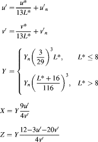
The colour difference between two points in either the L∗a∗b∗ or L∗u∗v∗ colour space may be determined by calculating the Euclidean distance between the corresponding vectors.
6.3.3 Colour Thresholding
Colour thresholding, like scalar thresholding, assigns a label to each pixel. With colour images, the purpose is to detect which pixels belong to each of a set of colours of interest. The output of colour thresholding is an image of labels, with each label corresponding to a colour class.
A computationally simple approach is to associate a rectangular box in the colour coordinates with a colour class. This corresponds to using a pair of thresholds for each component to define the boundaries of the box along that component.
It is generally not appropriate to use RGB space for this unless the illumination is fixed. This is because there is a strong correlation between the red, green and blue components, and all three will scale with illumination. This means that as the intensity changes, points will move diagonally in RGB space, requiring the box to be large. Consequently, only a few very different colours can be detected, and there is poor discrimination between colours.
Converting to YCbCr will give some improvement because rectangular boxes aligned with the YCbCr axes will be diagonal in RGB space. However, the chrominance components still scale with the luminance. Better discrimination may be obtained by scaling the chrominance by the luminance, or alternatively scaling the chrominance components by the maximum of the red, green and blue components (Johnston et al., 2005b).
Alternatively, the thresholding may be performed directly in the HSV colour space where the hue and saturation are independent of the luminance. Note that the HLS colour space is usually less suitable than HSV because the saturation changes with lightness when the lightness is greater than 50%.
The implementation of colour thresholding extends the contouring operation of Equation 6.8 and Figure 6.14 to each of the three channels, as shown in the left in Figure 6.42. This circuit will need to be repeated for each colour class to be detected.
Figure 6.42 Colour thresholding. Left: comparisons required for each colour class using a rectangular block; right: lookup table approach, with one lookup table per colour channel, detects multiple classes in parallel.
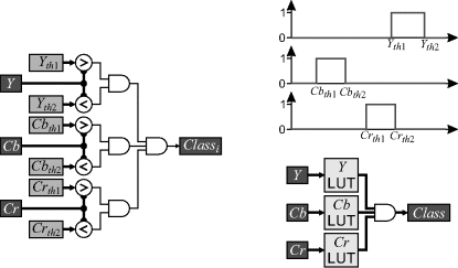
An alternative is to use a lookup table to implement the thresholding. This requires a separate LUT for each channel, but has the advantage that multiple classes may be segmented simultaneously by having a separate bit-plane associated with each colour class in the lookup tables (Sen Gupta et al., 2004).
The set of pixel values corresponding to a colour class do not necessarily need to fall within a rectangular box aligned with the component axes. However, the logic becomes increasingly more complex to handle arbitrary shaped regions. One approach is to use a single large lookup table taking as input the concatenated components of the colour input vector (Sen Gupta et al., 2003). The mapping can then be arbitrarily complex and can include any necessary colour space conversions. Unfortunately, such a lookup table is prohibitively large (224 = 16 777 216 entries for 24-bit colour) and would need to be implemented in external memory. The table size may be reduced by using fewer bits of the input at the cost of poorer discrimination.
A composite approach can also be used. For example, Johnston et al. (2005a) use two lookup tables, for each of ![]() and
and ![]() , and combine the normalisation division by
, and combine the normalisation division by ![]() into those tables, with a reduced number of bits. The resultant tables had only 512 entries of four bits (for four colour classes) enabling both tables to be contained within a single 4 Kbit block RAM.
into those tables, with a reduced number of bits. The resultant tables had only 512 entries of four bits (for four colour classes) enabling both tables to be contained within a single 4 Kbit block RAM.
6.3.4 Colour Correction
The colour of each pixel observed in an image depends not only on the spectral reflectivity of the corresponding object point, but also on the illumination. For example, the colours of objects within a scene illuminated by incandescent light can be quite different from those illuminated by fluorescent light. For outdoor scenes, the spectral characteristics of the illumination depend on whether the object is illuminated by sunlight, or in shadow, or whether the sky is clear or overcast, or even on the time of day.
The colour constancy problem is that of estimating how the scene would appear given canonical illumination. Unfortunately, without prior knowledge of the illumination, this is an ill-posed problem. In practise, it is not necessary to estimate the full spectral characteristics of the illumination; it is sufficient to remove the effects of varying illumination on the image. Colour correction involves transforming the RGB value of each pixel in the image to remove the effects of illumination. In general, this requires determining the components of a 3 × 3 linear transformation matrix. However, given that the spectral distribution at the sensor is the product of the reflectivity and illumination distributions, this is often simplified to a diagonal matrix, independently scaling the ![]() ,
, ![]() , and
, and ![]() components (Finlayson et al., 1994). Note that if any of the components are saturated, this will result in an additional colour change that cannot easily be corrected.
components (Finlayson et al., 1994). Note that if any of the components are saturated, this will result in an additional colour change that cannot easily be corrected.
Perhaps the simplest model is to assume that, on average, the image is achromatic (Finlayson et al., 2001). This implies that the average colour within the image should be grey. The effective illumination colour is then given by the mean of the red, green and blue components of the image. Correction is performed by dividing by the mean value and scaling to ensure that all pixel values are within the range of allowed values.

where ![]() are the corrected colour components and the scaling factor,
are the corrected colour components and the scaling factor, ![]() , that maximises the output contrast is given by:
, that maximises the output contrast is given by:
(6.87) 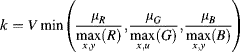
where ![]() . Alternatively, the scaling factor can be set to
. Alternatively, the scaling factor can be set to ![]() (Funt et al., 1998), although this has the danger that one or more of the components may saturate.
(Funt et al., 1998), although this has the danger that one or more of the components may saturate.
The major limitation of this approach is that if the image contains a dominant colour, the estimate of the illumination colour will be biased towards that colour (Gershon et al., 1987). As a result, a colour cast complementary to the dominant colour will be introduced into the image. This is clearly seen in the centre panel of Figure 6.43, where a bluish cast is introduced. As it is not known in general whether or not there is a dominant colour, this approach to colour correction is impractical.
Figure 6.43 Simple colour correction. Left: original image captured under incandescent lights, resulting in a yellowish-red cast; centre: correcting assuming the average is grey, using Equation 6.86; right: correcting assuming the brightest pixel is white, using Equation 6.88. (See colour version of this figure in colour plate Section)
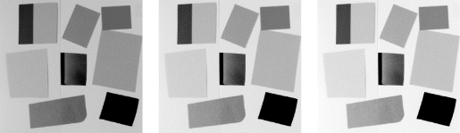
Another assumption that is sometimes used for colour correction is that the image contains at least one white pixel within the image, and that the white region is the brightest in the image. In this case, the white pixel may be found simply by finding the maximum of each component. Since this should be white (achromatic, with all components equal), the input image can be corrected by scaling each component by its corresponding maximum (Funt et al., 1998):
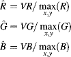
The results of this scheme are shown in the right panel of Figure 6.43.
One limitation of this approach is that it is easy for the assumptions to be violated. If the white pixel is the brightest in the image, there is a strong possibility that one or more of the channels will be saturated at ![]() . The true value of that component will be underestimated, affecting the correction. In many cases, the brightest point in an image is the result of specular reflection with the resulting pixel affected by the colour of the reflecting surface. Also, basing the correction on a single pixel will inevitably introduce noise into the estimate of the illumination colour, affecting the accuracy of any correction. These limitations may be mitigated by requiring a region of adjacent pixels be detected, and using the mean of that region. The logic for detection, however, becomes considerably more complex.
. The true value of that component will be underestimated, affecting the correction. In many cases, the brightest point in an image is the result of specular reflection with the resulting pixel affected by the colour of the reflecting surface. Also, basing the correction on a single pixel will inevitably introduce noise into the estimate of the illumination colour, affecting the accuracy of any correction. These limitations may be mitigated by requiring a region of adjacent pixels be detected, and using the mean of that region. The logic for detection, however, becomes considerably more complex.
The brightest object in the image may not be white, and if it is white it may not be pure white. If the colour is slightly off-white, making it white will introduce a cast. This limitation is harder to overcome, because it is impossible to distinguish between an off-white surface or slightly coloured illumination.
This approach may be extended by deliberately placing a white patch within the image. If the illumination and camera settings do not change with time, this may even be captured off-line as a calibration image. The white patch can then be detected either automatically, or by having the patch in a known location, or by manually selecting the region of interest. Let ![]() be the mean of the pixels within the white patch, then the correction may be performed as:
be the mean of the pixels within the white patch, then the correction may be performed as:

If the white patch is not the brightest region within the image (for example, a light grey is used instead to prevent any of the components of the calibration patch from saturating), then the ![]() in Equation 6.89 may be replaced by
in Equation 6.89 may be replaced by ![]() similar to Equation 6.86.
similar to Equation 6.86.
This will ensure that the white patch will appear achromatic. However, the camera may also introduce a DC offset in the output (for example as an offset in the amplifier or A/D converter, or not completely estimating the dark current). The colour correction may be enhanced by introducing a black patch into the model. Let ![]() be the mean of the pixels within the black patch. A colour correction using both patches is:
be the mean of the pixels within the black patch. A colour correction using both patches is:
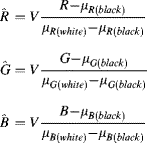
The results of this correction are shown in the centre panel of Figure 6.44.
Figure 6.44 Correcting using black, white and grey patches. Left: original image with the patches marked; centre: stretching each channel to correct for black and white, using Equation 6.90; right: adjusting the gamma of the red and blue channels using Equation 6.91 to make the grey patch grey. (See colour version of this figure in colour plate Section)
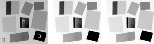
If the calibration performed off-line, then the colour correction is making a brightness and contrast adjustment to each of the channels, as described in Section 6.1.1. If the calibration is performed on-line, then the best approach is to place the black and white patches at the top of the image, so the mean values may be used to correct the rest of the image. Otherwise, the whole image needs to be stored in a frame buffer to enable the whole image to be corrected. If the illumination is changing slowly, then it may be sufficient to use the channel gains and offsets calculated from the previous frame.
A more sophisticated model adds a third mid-grey patch, with mean value ![]() . This allows slight variations in gamma to be corrected between the channels. The green pixel value is left unchanged, but a gamma correction is applied to the red and blue channels to make the components equal for the grey patch. Considering just the red component (a similar equation results for blue):
. This allows slight variations in gamma to be corrected between the channels. The green pixel value is left unchanged, but a gamma correction is applied to the red and blue channels to make the components equal for the grey patch. Considering just the red component (a similar equation results for blue):
(6.92) 
The results of adjusting the gamma are shown in the right panel of Figure 6.44.
Correcting for grey requires the addition of two gamma correction blocks, one for each of red and blue as shown in Figure 6.45. The circuit for these is complicated by the fact that the gamma values are not constant, but are a result of calibration. If implemented on-line, the calculation of the gamma is also required. However, since this is only performed once per frame, it is probably best implemented in software rather than directly in hardware. In that case, the software can also calculate the values for a lookup table implementation of the gamma correction blocks.
Figure 6.45 Implementing colour correction; the various parameters are stored in registers. Overflow detection and clipping has been omitted for clarity.
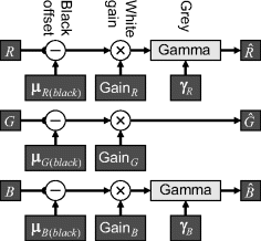
There is a wide range of more complex illumination estimation methods, which are not considered here. Several of these are discussed elsewhere (Funt et al., 1998; Finlayson et al., 2001).
6.3.5 Colour Enhancement
When performing colour enhancement, is often easier to work in HSV or HLS space. Since the hue represents the basic colour, generally it is left unchanged (unless correcting colour errors as described above). Colours can be made move vivid by increasing the saturation. This can be achieved by multiplying by a constant, or using a gamma enhancement (with ![]() ). Overall the contrast of the image may be enhanced by enhancing the lightness or value component.
). Overall the contrast of the image may be enhanced by enhancing the lightness or value component.
Point operations are some of the simplest to implement on an FPGA because each output pixel value depends only on the corresponding input pixel value. This enables them to be implemented using any processing mode. Since there are no dependencies between pixels, point operations can readily be parallelised by building multiple processing units. It is also common to pipeline point operations, processing data as it is being read from or written to memory.
Point operations on a single image are primarily concerned with adjusting the brightness or contrast (or equivalently adjusting the colour balance or contrast of a colour image). Thresholding is another common point operation, used for segmenting an image on the basis of intensity or colour. Any point operation may be directly implemented using a lookup table, giving constant processing time regardless of the complexity of the operation.
Point operations may also be applied between multiple images. Virtually any operation may be applied between the pixels of the images being combined. Most commonly, these are images captured at different times, so requires frame buffering to store the history. A common architecture is recursive processing, where a newly acquired image is combined with one or more images held in a frame buffer, with the result written back to the frame buffer.
The simplicity of point operations is also one of the main limitations. Frequently, global data is required to set appropriate parameters (for example for contrast stretching or selecting an appropriate threshold level). The use of histograms to capture and derive some of these parameters is described in the next chapter. A point operation considers each pixel in isolation and does not take into account context. Local filters, where the output pixel value is dependent on several pixels within a local neighbourhood, are described in Chapter 8.