Figure 6.28 Temporal false colouring. Images taken at different times are assigned to different channels, with the resultant output showing coloured regions where there are temporal differences.

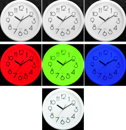
Figure 6.29 Pseudocolour or false colour mapping using lookup tables.

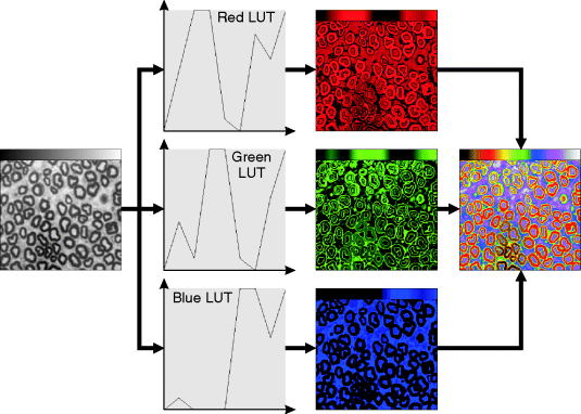
Figure 6.30 RGB colour space. Top left: combining red, green and blue primary colours; bottom: the red, green and blue components of the colour image on the top right.

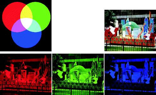
Figure 6.32 CMY colour space. Top left: combining yellow, magenta and cyan secondary colours; bottom: the yellow, magenta and cyan components of the colour image on the top right.

Figure 6.34 YCbCr colour space. Top left: the Cb–Cr colour plane at mid luminance; bottom: the luminance and chrominance components of the colour image on the top right.

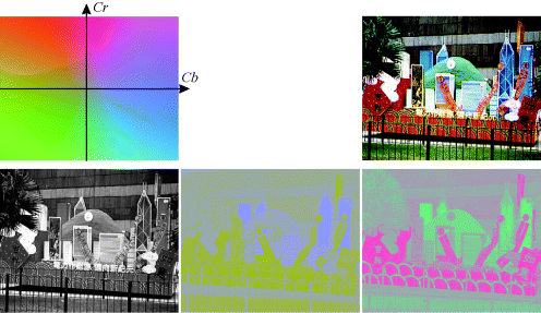
Figure 6.36 HSVand HLS colour spaces. Left: the HSV cone; centre: the HLS bi-cone; right: the hue colour wheel.

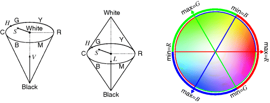
Figure 6.37 HSVand HLS colour spaces. Top left: HSV hue colour wheel, with saturation increasing with radius; middle row: the HSV hue, saturation and value components of the colour image on the top right; bottom row: the HLS hue, saturation and lightness components.

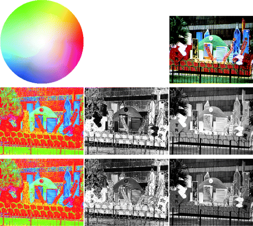
Figure 6.40 Chromaticity diagram. The numbers are wavelengths of monochromatic light in nanometres.

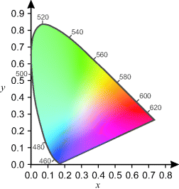
Figure 6.41 Device dependent r–g chromaticity.

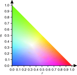
Figure 6.43 Simple colour correction. Left: original image captured under incandescent lights, resulting in a yellowish-red cast; centre: correcting assuming the average is grey, using Equation 6.86; right: correcting assuming the brightest pixel is white, using Equation 6.88.

Figure 6.44 Correcting using black, white and grey patches. Left: original image with the patches marked; centre: stretching each channel to correct for black and white, using Equation 6.90; right: adjusting the gamma of the red and blue channels using Equation 6.91 to make the grey patch grey.

Figure 7.24 Using a two-dimensional histogram for colour segmentation. Left: U–V histogram using Equation 6.61; centre: after thresholding and labelling, used as a two-dimensional lookup table; right: segmented image.