
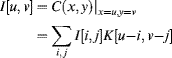
Chapter 9
Geometric Transformations
The next class of operations to be considered is that of geometric transformations. These redefine the geometric arrangement of the pixels within an image (Wolberg, 1990). Examples of geometric transformations include zooming, rotating and perspective transformation. Such transformations are typically used to correct spatial distortions resulting from the imaging process, or to normalise an image by registering it to a predefined coordinate system (for example, registering an aerial image to a particular map projection or warping a stereo pair of images so that the rows corresponds to epipolar lines).
Unlike point operations and local filters, the output pixel does not, in general, come from the same input pixel location. This means that some form of buffering is required to manage the delays resulting from the changed geometry. The simplest approach is to hold the input image or the output image (or both) in a frame buffer. Most geometric transformations cannot easily be implemented with streaming for both the input and output.
The mapping between input and output pixels may be defined in two different ways, as illustrated in Figure 9.1. The forward mapping defines the output pixel coordinates, ![]() , as a function,
, as a function, ![]() , of the input coordinates:
, of the input coordinates:
(9.1) ![]()
Figure 9.1 Forward and reverse mappings for geometric transformation.
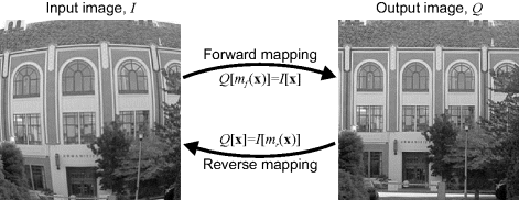
The forward mapping is suitable for processing a streamed input, for example from a camera, because it specifies for each input pixel, where the pixel value goes to in the output image. Therefore, it is able to process sequential addresses in the input image. Note that as a result of the mapping, sequential input addresses do not necessarily correspond to sequential output addresses.
Conversely, the reverse mapping defines the input pixel coordinates as a function, ![]() , of the output coordinates:
, of the output coordinates:
(9.2) ![]()
It is, therefore, more suited for producing a streamed output, for example images being streamed to a display, because for each output pixel the reverse mapping specifies where the pixel value comes from in the input image. It can therefore process sequential output addresses, but will in general require non-sequential access of the input image.
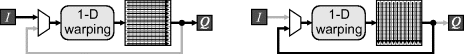
The basic architectures for implementing forward and reverse mappings are compared in Figure 9.2. For streamed access of the input (forward mapping) or output (reverse mapping), the address will be provided by appropriate counters synchronised with the corresponding stream. While the input to the mappings will usually be integer image coordinates, the mapped addresses will not, in general, be integer locations. Consequently, the implementation will be more complex than that implied by Figure 9.2. The main issues associated with the forward and reverse mappings are different, so are discussed here in more detail separately.
Figure 9.2 Basic architectures for geometric transformation. Left: forward mapping; right: reverse mapping.

With a forward mapping, simply rounding the output coordinates to the nearest pixel results in two problems. Firstly, if the transform magnification is greater than one (zooming in), there can be holes in the output image, where no input pixels map to. Such output pixels will not be assigned a value. Secondly, if the magnification is less than one (zooming out), several input pixels can map onto a single output pixel. If the input pixel value is simply written to the frame buffer, then the value may be overwritten by subsequent pixels. Even if the magnification is exactly one, if there is a rotation then both problems can occur, as demonstrated in the left panel of Figure 9.3.
Figure 9.3 Problems with forward mapping. Left: the input pixels (dots) are rotated anti-clockwise by 40 degrees. Output pixels shaded dark have no input pixels mapping to them. Output pixels shaded light are mapped to by two input pixels. Right: it is necessary to map the whole pixel to avoid such problems.
To overcome both problems, it is necessary to map the whole rectangular region associated with each input pixel to the output image. Each output pixel is then given by the weighted sum of all the input pixels which overlap it. The weight associated with each pixel is given by the proportion of the output pixel that is contributed to by the corresponding input pixel:
(9.3) ![]()
where
For this, it is easier to map the corners of the pixel, because these define the edges, which in turn define the region occupied by the pixel. On the output, it is necessary to maintain an accumulator image to which fractions of each input pixel are added as they are streamed in. There are two difficulties with implementing this approach on an FPGA for a streamed input. Firstly, each input pixel can intersect many output pixels, especially if the magnification of the transform is greater than one. Therefore, many (depending on the position of the pixel and the magnification) clock cycles are required to adjust all of the output pixels affected by each input pixel. Since each output pixel may be contributed to by several input pixels, a complex caching arrangement is required to overcome the associated memory bandwidth bottleneck. A second problem is that, even for relatively simple mappings, determining the intersection as required by Equation 9.4 is both complex and time consuming.
9.1.1 Separable Mapping
Both of these problems may be significantly simplified by separating the transformation into two stages or passes (Catmull and Smith, 1980). The key is to operate on each dimension separately:
(9.5) ![]()
The first pass through the image transforms each row independently to get each pixel on that row into the correct column. This forms the temporary intermediate image, ![]() . The second pass then operates on each column independently, getting each pixel into the correct row. This process is illustrated with an example in Figure 9.4. The result of the two transformations is that each pixel ends up in the desired output location. Note that the transformation for the second pass is in terms of u and y rather than x and y to reflect the results of the first pass.
. The second pass then operates on each column independently, getting each pixel into the correct row. This process is illustrated with an example in Figure 9.4. The result of the two transformations is that each pixel ends up in the desired output location. Note that the transformation for the second pass is in terms of u and y rather than x and y to reflect the results of the first pass.
Figure 9.4 Two-pass transformation to rotate an image by 40 degrees. Left: input image; centre: intermediate image after transforming each row; right: transforming each column.
Reducing the transformation from two dimensions to one dimension significantly reduces the difficulty in finding the pixel boundaries. In one dimension, each pixel has only two boundaries: with the previous pixel and with the next pixel. The boundary with the previous pixel can be cached from the previous input pixel, so only one boundary needs to be calculated for each new pixel.
Both the input and output from each pass are produced in sequential order, enabling stream processing to be used. Although the second pass scans down the columns of the image, stream processing can still be used. However, a frame buffer is required between the two passes to hold the intermediate image. If the input is streamed from memory, and the bandwidth enables, the image can be processed in place, with the output written back into the same frame buffer. Bank switching is still required to process every frame, with an implementation is shown in Figure 9.5. One frame buffer bank is used for each pass, with the banks switched each frame to maintain the throughput. The processing latency is a little over two frame periods.
Figure 9.5 Implementation of two-pass warping with forward mapping using bank switching.
Since the same algorithm is applied to both the rows and columns (apart from calculating the mapping), a single one-dimensional processor may be used for both passes, as shown in Figure 9.6. This halves the resource requirements at the expense of only processing every second input frame.
Figure 9.6 Two-pass forward mapping. Left: in the first pass each row is warped and written to a frame buffer, while the previous image is streamed out; right: in the second pass, each column is processed and written back to the frame buffer.
Since each row and column is processed independently, the algorithm may be accelerated by processing multiple rows and columns in parallel. The main limitation on the number of rows that may be processed in parallel is the bandwidth available to the frame buffer.
Before looking at the implementation of the one-dimensional warping, the limitations of the two-pass approach will be discussed. Firstly, consider rotating an image by 90 degrees – all of the pixels on a row in the input will end up in the same column in the output. Therefore, the first pass maps all of the points on a row to the same point in the intermediate image. The second pass is then supposed to map each of these points onto a separate row in the output image, but is unable to because all the data has been collapsed to a point. This is called the bottleneck problem and occurs where the local rotation is close to 90 degrees. Even for other angles, there is a reduction in resolution as a result of the compression of data in the first pass, followed by an expansion in the second pass (Figure 9.4 shows an example – the data in the intermediate image occupies a smaller area than either the input or output images). The worst cases may be overcome by rotating the image 90 degrees first, and then performing the mapping. This is equivalent to treating the incoming row-wise scanned data as a column scan and performing the column mapping first. This works fine for global rotations. However, many warps may locally have a range of rotation angles, in which case some parts of the image should be rotated first and others should not. Wolberg and Boult (1989) overcame this by performing both operations in parallel and selected the output locally based on which had the least compression in the intermediate image. This solution comes at the cost of doubling the hardware required (in particular the number of frame buffers needed).
An alternative algorithm that avoids the bottleneck problem when performing rotations is to use three passes rather than two, with each pass a shear transformation (Wolberg, 1990). While requiring an extra pass through the image, it has the advantage that each pass merely shifts the pixels along a row or column, resulting in a computationally very simple implementation for pure rotations.
A second problem occurs if the mappings on each row or column in the first pass are not either monotonically increasing or decreasing. As a result, the mapping is many-to-one, with data from one part of the image folding over that which has already been calculated. (Such fold-over can occur even if the complete mapping does not fold over; the second pass would map the different folds to different rows.) In the original proposal (Catmull and Smith, 1980), it was suggested that such fold-over data from the first pass be held in additional frame buffers, so that it is available for unfolding in the second pass. Without such additional resources, the range of geometric transformations that may be performed using the two-pass approach is reduced.
A third difficulty with the two-pass forward mapping is that the second transformation is in terms of u and y. Since the original mapping is in terms of x and y, it is necessary to be able to invert the first mapping in order to derive the second mapping. Consider, for example, an affine transformation:
The first pass is straight forward, giving u in terms of x and y. However, v is also specified in terms of x and y rather than u and y. Inverting the first mapping gives:
(9.7) ![]()
and then substituting into the second part of Equation 9.6 gives the required second mapping:
(9.8) ![]()
While inverting the first mapping in this case is straightforward, for many mappings it can be difficult (or even impossible) to derive the mapping for the second pass and, even if it can be derived, it may be computationally expensive to perform. Wolberg and Boult (1989) overcame this by saving the original x in a second frame buffer, enabling ![]() from Equation 9.6 to be used. They also took the process one step further and represented the transformation through a pair of lookup tables rather than directly evaluating the mapping function.
from Equation 9.6 to be used. They also took the process one step further and represented the transformation through a pair of lookup tables rather than directly evaluating the mapping function.
The final issue is that the two-pass separable warp is not identical to the two-dimensional warp. This is because each one-dimensional transformation is of an infinitely thin line within the image. However, this line actually consists of a row or column of pixels with a thickness of one pixel. Since each row and column is warped independently, significant differences in the transformations between adjacent rows can lead to jagged edges (Wolberg and Boult, 1989). As long as adjacent rows (and columns) are mapped to within one pixel of one another, this is not a significant problem.
Subject to these limitations, the two-pass separable approach provides an effective approach to implement the forward mapping. Each pass requires the implementation of a one-dimensional geometric transformation. While the input data can simply be interpolated to give the output, this can result in aliasing where the magnification is less than one. To reduce aliasing, it is necessary to filter the input; in general this filter will be spatially variant, defined by the magnification at each point.
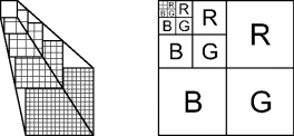
The filtering, interpolation and resampling can all be performed in a single operation (Fant, 1986). Fant's original algorithm used a reverse map; it was adapted by Wolberg et al. (2000) to use both the forward and reverse map, with the forward map presented in Figure 9.7. The basic principle is to maintain two fractional valued pointers into the stream of output pixels. Inseg indicates how many output pixels that the current input pixel has yet to cover, while Outseg indicates how much of the current output pixel remains to be filled. If Outseg is less than or equal to Inseg, an output pixel can be completed so an output cycle is triggered. The input value is weighted by Outseg, combined with the output value accumulated so far in Accum, and is output. The accumulator is reset, Outseg reset to one and Inseg decremented by Outseg to reflect the remaining input to be used. Otherwise Inseg is smaller, so the current input is insufficient to complete the output pixel. This triggers an input cycle, which accumulates the remainder of the current input pixel (weighted by the fraction of output pixel it covers), subtracts Inseg from Outseg to reflect the fraction of the output pixel remaining, and reads a new input pixel value. As each input pixel is loaded, the address is passed to the forward mapping function to get the corresponding pixel boundary in the output. The mapping may either be implemented directly or via a lookup table (Wolberg and Boult, 1989). The magnification or scale factor for the current pixel is obtained by subtracting the previous pixel boundary, OutPos, from the new boundary. This result is used to initialise Inseg.
Figure 9.7 One-dimensional warping using resampling interpolation.
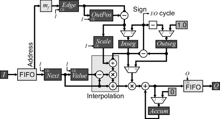
The interpolation block is required when the magnification is greater than one, to prevent a single pixel from simply being replicated in the output, resulting in large flat areas and contouring (Fant, 1986). It performs a linear interpolation between the current input value and the next pixel value in proportion to how much of the input pixel is remaining.
Each clock cycle is either an input cycle or an output cycle, although in general these do not alternate. (If the magnification is greater than one, then there will be multiple output pixels for each input pixel, and if the magnification is less than one, then there will be multiple input pixels for each output pixel.) A FIFO buffer is therefore required on both the input and output to smooth the flow of data to allow streaming with one pixel per clock cycle. Although the one-dimensional warping has an average latency of one row, it requires two row times to complete. Therefore, to run at pixel clock rates, two such warping units must be operated in parallel.
Handling of the image boundaries is not explicitly shown in Figure 9.7. The initial and trailing edge of the input can be detected from the mapping function. If the first pixel is already within the image, a series of empty pixels need to be output. Similarly, at the end of the input row, a series of empty pixels may also be required to complete the output row.
The speed can be significantly improved by combining the input and output cycles if the input pixel is sufficiently wide to also complete an output pixel (Wolberg et al., 2000). This will be the case if:
(9.9) ![]()
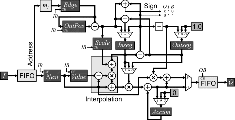
For the combined cycle, the clock is enabled for both (B) the input and output circuits. The extra logic to complete this is shown in Figure 9.8. The main change is rather than add the remainder of the old input pixel to an accumulator, the sum is added to the fraction of the new pixel required to complete the output, with the result sent directly to the FIFO.
Figure 9.8 Extending Figure 9.7 to combine the input and output cycle (labelled B for both) if possible.
While many mappings will still take longer than one data row length, the extra time required is small in most cases. Where the magnification is greater than one, a pixel will be output every clock cycle, with an input cycle when necessary to provide more data. The converse will be true where the magnification is less than one. Assuming that the input and output are the same size, then extra clock cycles are only required when the magnification is greater than one on some parts of the row, and less than one on other parts. If the image has horizontal blanking at the end of each row, this would be sufficient to handle most mappings in a single row time.
Since the output pixel value is a sum over a fraction of pixels, Evemy et al. (1990) took a different approach to accelerate the mapping by completely separating the input and output cycles. As the row is input, the image is integrated to create a sum table. This enables any output pixel to be calculated by taking the difference between the two interpolated entries into the sum table corresponding to the edges of the output pixel. After the complete row has been loaded, the output phase begins. The reverse mapping (along the row) is used to determine the position of the edge of the output pixel in the sum table, with the subpixel position determined through interpolation (Figure 5.31). The difference between successive input sums gives the integral from the input corresponding to the output pixel. This is normalised by the width of the output pixel to give the output pixel value. The structure for this is shown in Figure 9.9.
Figure 9.9 Separating the input and output phases using sum tables, and interpolating on the output.
As both input and output take exactly one clock cycle per pixel, regardless of the magnification, this approach can be readily streamed. By bank switching the summed row buffers, a second row is loaded while the first row is being transformed and output. The latency of this scheme is, therefore, one row length (plus any pipeline latencies). Since the block RAMs on FPGAs are dual-port, a single memory with length of two rows can be used, with the bank switching controlled by the most significant address line.
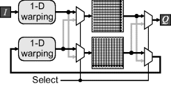
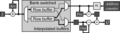
Rather than perform the two passes independently, as implied at the start of this section, the two passes can be combined together (Bailey and Bouganis, 2009a). In the second pass, rather than process each column separately, they can be processed in parallel, with row buffers used to hold the data. The basic idea is illustrated in Figure 9.10.
Figure 9.10 Combining the row and column warps by implementing the column warps in parallel.
The circuit for the first pass row warping can be any of those described above. For the second pass, using sum tables would require an image buffer because the complete column needs to be input before output begins, gaining very little. However, with the interleaved input and output methods, each time a pixel is output from the first pass, it may be passed to the appropriate column in the second pass. Any output pixel from the second pass may be saved into the corresponding location in the output frame buffer. If the magnification is less than one, then at most one pixel will be written every clock cycle. Note that, in general, pixels will be written to the frame buffer non-sequentially because the mappings for each column will be different.
If the magnification is greater than one, then multiple clock cycles may be required to ready the column for the next input pixel before moving onto the next column. This will require that the column warping controls the rate of the row warping. If the input FIFO is not blocking, then it will also control the rate of the input stream.
To summarise, a forward mapping allows data to be streamed from an input. To save having to maintain an accumulator image, with consequent bandwidth issues, the mapping can be separated into two passes. The first pass operates on each row and warps each pixel into the correct column, whereas the second pass operates on each column, getting each pixel into the correct row.
In contrast, the reverse mapping determines for each output pixel where it comes from in the input image. This makes the reverse mapping well suited for producing a streamed output for display or passing to downstream operations. Reverse mapping is the most similar to software, where the output image is scanned and the output pixel obtained from the mapped point in the input image.
There are two factors which complicate this process. The first is the fact that the mapped coordinates do not necessarily fall on the input pixel grid. This requires some form of interpolation to calculate the pixel value to output. Interpolation methods are described in more detail in the next section. The second factor is that the when the magnification is less than one, it is necessary to filter the input image to reduce the effects of aliasing. If the magnification factor is constant (or approximately constant) then a simple filter may be used. However, if the magnification varies significantly with position (for example with a perspective transformation) then the filter must be spatially variant, with potentially large windows in some places in the image. Filtering the input image with a large window is also inefficient, because a conventional filter will produce outputs corresponding to every input pixel position. The small magnification means that most of the calculated outputs will be discarded anyway.
As there is insufficient time to perform the filtering while producing the output, it is necessary to prefilter the image before the geometric transformation. There are two main approaches to filtering that allow for a range of magnifications. One is to use a pyramidal data structure with a series of filtered images at a range of resolutions; the other is to use summed area tables.
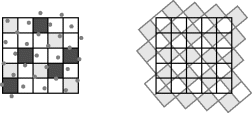
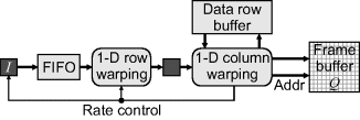
An image pyramid is a multiresolution data structure used to represent an image at a range of scales. Each level of the pyramid is formed by successively filtering and down-sampling the layer below it by a factor of two, as illustrated in Figure 9.11. Typically, each pixel in the pyramid is the average of the four pixels below it. A pyramid can be constructed in a single pass through the image and requires 33% more storage than the original image. A convenient memory organisation for a colour image is a mip-map (Williams, 1983), which divides the image memory into four quadrants, one for each of red, green, and blue, and the fourth quadrant for the remainder of the pyramid at the higher levels as shown on the right in Figure 9.11.
Figure 9.11 Pyramidal data structures. Left: multiresolution pyramid; right: mip-map organisation for storing colour images (Williams, 1983).
The pyramid can be used for filtering for geometric transformation in several ways. The simplest is to determine which level corresponds to the desired level of filtering based on the magnification, and select the nearest pixel within that level (Wolberg, 1990). The limitation of this is that the filter window is considered to be a square, with size and position determined by pyramid structure. This may be improved by interpolating within the pyramid (Williams, 1983) in the x, y, and scale directions (tri-linear interpolation). Such interpolation requires reading eight locations in the pyramid, requiring innovative mapping and caching techniques to achieve in a single clock cycle.
An alternative approach is to use summed area tables (Crow, 1984). A summed area image is formed in which each pixel contains the sum of all of the pixels above and to the left of it:
(9.10) ![]()
The sum over any arbitrary rectangular region may then be calculated in constant time (with four accesses to the summed area table, as shown in Figure 9.12) regardless of the size and position of the rectangular region:
Figure 9.12 Left: using a summed area table to find the sum of pixel values within an arbitrary rectangular area; right: efficient streamed implementation to create a summed area table.
Summed area tables can be created recursively by inverting Equation 9.11:
This requires a row buffer to hold the sums from the previous row. A more efficient approach, however, is to maintain a column sum and add this to the sum:
as shown on the right in Figure 9.12. In the first row of the image, the previous column sum is initialised as 0 (rather than feeding back from the row buffer) and, in the first column, the sum table for the row is initialised to 0. Two benefits of using Equation 9.13 rather than Equation 9.12 are that it reduces the number of operations and the row buffer can be narrower, since the column sum requires fewer bits per pixel than the area sum.
To use the summed area table for filtering requires dividing the sum from Equation 9.11 by the area to give the output pixel value. This can be seen as an extension of box filtering, as described in Section 8.2, to allow filtering with a variable window size.
In the context of filtering for geometric transformation, summed area tables have an advantage over pyramid structures in that they give more flexibility to the shape and size of the window. Note that with magnifications close to and greater than one, filtering is not necessary, and the input pixel values can simply be interpolated to give the required output.
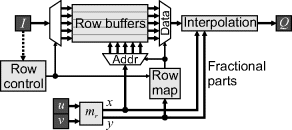
Although an arbitrary warp requires the complete input image to be available for the reverse mapping, if the transformation keeps the image mostly the same (for example, correcting lens distortion or rotating by a small angle), then the transformation can begin before the whole image is buffered. Sufficient image rows must be buffered to account for the shift in the vertical direction between the input and output images. While a new input row is being streamed in, the output is calculated and streamed from the row buffers, as shown in Figure 9.13. The use of dual-port row buffers enables direct implementation of bilinear interpolation. Address calculations (to select the appropriate row buffer) are simplified by having the number of row buffers be a power of two, although this may be overcome by using a small lookup table to map addresses to row buffers. Reducing the number of row buffers required can significantly reduce both resource requirements and the latency (Akeila and Morris, 2008).
Figure 9.13 Reverse mapping with a partial frame buffer (using row buffers).
When transforming the image using the reverse map, the mapped coordinates are usually not on integer locations. Estimating the output pixel value requires estimating the underlying continuous intensity distribution and resampling this at the desired locations. The underlying continuous image, ![]() , is formed by convolving the input image samples with a continuous interpolation kernel,
, is formed by convolving the input image samples with a continuous interpolation kernel, ![]() :
:
which is illustrated in one dimension in Figure 9.14.
Figure 9.14 Interpolation process. Top: the input samples are convolved with a continuous interpolation kernel; middle: the convolution gives a continuous image; bottom: this is then resampled at the desired locations to give the output samples.
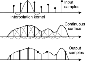
If the images are band-limited and sampled at greater than twice the maximum frequency, then the continuous image may be reconstructed exactly using a sinc kernel. Unfortunately, the sinc kernel has infinite extent and only decays slowly. Instead, simpler kernels with limited extent (or region of support) that approximate the sinc are used. This is important because it reduces the bandwidth required to access the input pixels.
Sampling the continuous image is equivalent to weighting a sampled interpolation kernel by the corresponding pixel value:
Resampling can, therefore, be seen as filtering the input image with the weights given by the sampled interpolation kernel. There are two important differences with the filtering described in Section 8.2. Firstly, the fractional part of the input location changes from one output pixel to the next, so too do the filter weights. This means that some of the optimisations based on filtering with constant weights can no longer be applied. Secondly, the path through the input image corresponding to a row of pixels in the output will not, in general, follow a raster scan, but will follow an arbitrary curve. This makes the simple, regular, caching arrangements for local filters unsuited for interpolation, and more complex caching arrangements must be devised to manage the oblique or curved path through the input image.
Nearest neighbour interpolation is the simplest form of interpolation; it simply selects the nearest pixel to the desired location. This requires rounding the coordinates into the input image to the nearest integer, which is achieved by adding 0.5 and selecting the integer component. If this addition can be incorporated into the mapping function, then the fractional component can simply be truncated from the calculated coordinates. The corresponding pixel in the input image can then be read directly from the frame buffer.
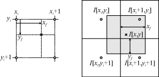
Other interpolation schemes combine the values of neighbouring pixels to estimate the value at a fractional position. The input pixel is split into its integer and fractional components
(9.16) ![]()
The integer parts of the desired location, ![]() , are used to select the input pixel values, which are weighted by values derived from the fractional components,
, are used to select the input pixel values, which are weighted by values derived from the fractional components, ![]() , as defined in Figure 9.15.
, as defined in Figure 9.15.
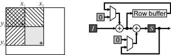
Figure 9.15 Left: coordinate definitions for interpolation; subscripts i and f denote integer and fractional parts of the respective coordinates. Right: bilinear interpolation.
As with image filtering, the logic also needs to appropriately handle boundary conditions. There are two specific cases that need to be handled. The first is when the output pixel does not fall within the input image. In this case, the interpolation is not required and an empty pixel (however this is defined for the application) is provided to the output. The second case is when the output pixel comes from near the edge of the input image and one or more of the neighbouring pixels are outside the image. It is necessary to provide appropriate values as input to the interpolation depending on the image extension scheme used.
9.3.1 Bilinear Interpolation
Perhaps the most commonly used interpolation method is bilinear interpolation. It combines the values of the four nearest pixels using separable linear interpolation:
An alternative way of interpreting Equation 9.17 is demonstrated on the right in Figure 9.15. Each pixel location is represented by a square, with the weights given by the area of overlap between the desired output pixel and the available input pixels. Although Equation 9.17 appears to require eight multiplications, careful factorisation to exploit separability can reduce this to three:
(9.18) 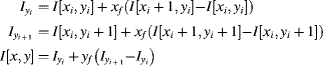
While a random access implementation (for example such as performed in software) is trivial, accessing all four input pixels within a single clock cycle requires careful cache design.
If the whole image is available on chip, it will be stored in block RAMs. By ensuring that successive rows are stored in separate RAMs, a dual-port memory can simultaneously provide both input pixels on each line, hence all four pixels, in a single clock cycle. If only a single port is available, the data must be partitioned with odd and even addresses in separate banks so that all four input pixels may be accessed simultaneously. In most applications, however, there is insufficient on-chip memory available to hold the whole image and the image is held in an external frame buffer with only one access per clock cycle.
In this case, memory bandwidth becomes the bottleneck. Each pixel should only be read from external memory once, and held in an on-chip cache for use in subsequent windows. There are two main approaches that can be used. One is to load the input pixels as necessary; the other is to preload the cache and always access pixels directly from there. Since the path through the input image does not, in general, follow a raster scan, it is necessary to store not only the pixel values but also their locations within the cache. However, to avoid the complexity of associative memory, the row address can be implicit in which buffer the data is stored in. Consider a B row cache consisting of B separate block RAMs. The particular block RAM used to cache a pixel may be determined by taking the row address modulo B and using this to index the cache blocks. This is obviously simplified if B is a power of two, where the least significant bits of the row address give the cache block.
Loading input pixels on demand requires that successive output rows and pixels be mapped sufficiently closely in the input image that the reuse from one location to the next is such that the required input pixels are available (Gribbon and Bailey, 2004). This generally requires that the magnification be greater than one. Otherwise multiple external memory accesses are required to obtain the input data. If the output stream has horizontal blanking periods at the end of each row, this requirement may be partially relaxed through using a FIFO buffer on the output to smooth the flow. For a bilinear interpolation, a new frame may be initialised by loading the first row twice; the first time loads data into the cache but does not produce output, while the second pass produces the first row of output. This is similar to directly priming the row buffers for a regular filter.
The requirements are relaxed somewhat in a multiphase design, because more clock cycles are available to gather the required input pixel values.
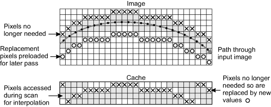
Preloading the cache is a little more complex. It may require calculating in advance which pixels are going to be required. This will mean either performing the calculation twice, once for loading the cache and once for generating the output, or buffering the results of the calculation for use when all of the pixels are available in the cache. These two approaches are compared in Figure 9.16. Another alternative is for the cache control to monitor when data is no longer required and automatically replace the expired values with new data. This relies on the progression of the scan through the image in successive rows, so that when a pixel is not used in a column it is replaced by the next corresponding pixel from the frame buffer. This process is illustrated in Figure 9.17.
Figure 9.16 Preloading the cache. Left: calculating the mapping twice – once for loading the cache and once for performing the interpolation; right: buffering the calculated mapping for when the data is available.
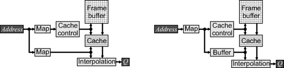
Figure 9.17 Preloading pixels which are no longer required.
9.3.2 Bicubic Interpolation
While bilinear interpolation gives reasonable results in many applications, a smoother result may be obtained through bicubic interpolation. Bicubic interpolation uses a separable piecewise cubic interpolation kernel with the constraints that it is continuous and has a continuous first derivative. These constraints result in the following kernel (Keys, 1981):
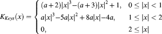
where a is a free parameter. Selecting ![]() makes the interpolated function agree with the Taylor series approximation to a sinc in as many terms as possible (Keys, 1981). The resulting one-dimensional interpolation weights two samples on either side of the desired data point, giving a region of support of four samples:
makes the interpolated function agree with the Taylor series approximation to a sinc in as many terms as possible (Keys, 1981). The resulting one-dimensional interpolation weights two samples on either side of the desired data point, giving a region of support of four samples:
where the weights may be derived by substituting the fractional part of the desired pixel location into Equation 9.19:
(9.21) 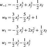
These weights may either be calculated directly from the fractional component or determined through a set of small lookup tables. Since the weights sum to one, Equation 9.20 may be simplified to reduce the number of multiplications:
(9.22) 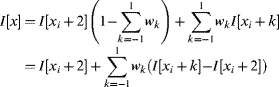
The implementation of the separable bicubic interpolation requires a total of 15 multiplications, as demonstrated in Figure 9.18. Here the filter weights are provided by lookup tables on the fractional component of the pixel.
Figure 9.18 Implementation of bicubic interpolation.

The larger region of support makes the design of the cache more complex for bicubic interpolation than for bilinear interpolation. In principle, the methods described above for bilinear interpolation may be extended, although memory partitioning is generally required to obtain the four pixels on each row within the window. The added complexity of memory management combined with the extra logic required to perform the filtering for a larger window make bilinear interpolation an acceptable compromise between accuracy and computational complexity in many applications.
Nuño-Maganda and Arias-Estrada (2005) use bicubic interpolation for image zooming. Since there is no rotation, the regular access pattern enables conventional filter structures to be used, although the coefficients change from one pixel to the next. Bellas et al. (2009) used bicubic interpolation to correct fisheye lens distortion, which requires a more complex access pattern within the image. They overcame the memory bandwidth by dividing the input image into overlapping tiles and preloading the image data for a complete tile into a set of block RAMs on the FPGA before processing that tile. The block RAMs then provide the required bandwidth to access all of the pixels needed to interpolate each output pixel.
9.3.3 Splines
A cubic spline is the next most commonly used interpolation technique. A cubic spline also defines a continuous signal that passes through the sample points as a series of piece-wise cubic segments, with the condition that both the first and second derivatives are continuous at each of the samples. This has the effect that changing the value of any point will affect the segments over quite a wide range. Consequently, interpolating with splines is not a simple convolution with a kernel, because of their wide region of support.
B-splines, on the other hand, do have compact support. They are formed from the successive convolution of a rectangular function, as illustrated in Figure 9.19. ![]() corresponds to nearest neighbour interpolation, while
corresponds to nearest neighbour interpolation, while ![]() gives linear interpolation, as described above.
gives linear interpolation, as described above.
Figure 9.19 B-splines.
The cubic B-spline kernel is given by:
(9.23) 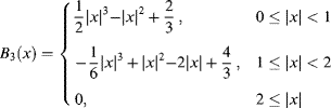
Its main limitation is that it does not go to zero at ![]() . This means that Equation 9.14 cannot be used directly for interpolation, since the continuous surface produced by convolving the image samples with the cubic B-spline kernel will not pass through the data points. Therefore, rather than weight the kernels with the image samples as in Equation 9.14, it is necessary to derive a set of coefficients based on the image samples:
. This means that Equation 9.14 cannot be used directly for interpolation, since the continuous surface produced by convolving the image samples with the cubic B-spline kernel will not pass through the data points. Therefore, rather than weight the kernels with the image samples as in Equation 9.14, it is necessary to derive a set of coefficients based on the image samples:
These coefficients may be derived by solving the inverse problem, by setting ![]() in Equation 9.24. Solving directly, this requires a matrix inversion, although this can be implemented using infinite impulse response filters in both the forward and backward direction on each row and column of the image (Unser et al., 1991). Spline interpolation therefore requires two stages, as shown in Figure 9.20: prefiltering the image to obtain the coefficients and then interpolation using the kernel. When implementing spline interpolation with an arbitrary (non-regular) sampling pattern, the prefiltering may be performed in the regularly sampled input image, with the result stored in the frame buffer. Then the interpolation stage may proceed as before, using the sampled kernel functions as filter weights to generate the output image.
in Equation 9.24. Solving directly, this requires a matrix inversion, although this can be implemented using infinite impulse response filters in both the forward and backward direction on each row and column of the image (Unser et al., 1991). Spline interpolation therefore requires two stages, as shown in Figure 9.20: prefiltering the image to obtain the coefficients and then interpolation using the kernel. When implementing spline interpolation with an arbitrary (non-regular) sampling pattern, the prefiltering may be performed in the regularly sampled input image, with the result stored in the frame buffer. Then the interpolation stage may proceed as before, using the sampled kernel functions as filter weights to generate the output image.
Figure 9.20 Structure for spline interpolation.
Direct implementation of the infinite impulse response prefiltering presents a problem for a streamed implementation, because each one-dimensional filter requires two passes, once in the forward direction and once in the reverse direction. However, since the impulse responses of these filters decay relatively quickly, they may be truncated and implemented using a finite impulse response filter (Ferrari and Park, 1997).
Rather than use B-splines, the kernel can be selected so that the coefficients of the prefilter are successively smaller powers of two (Ferrari and Park, 1997) (this has been called a 2-5-2 spline). This enables the filter to be implemented efficiently in hardware, using only shifts for the multiplications, as demonstrated on the left in Figure 9.21. Since each coefficient is shifted successively by one bit, shifting by more than k bits, where k is the number of bits used in the fixed-point representation of ![]() , will make the term go to zero. This provides a natural truncation point for the window.
, will make the term go to zero. This provides a natural truncation point for the window.
Figure 9.21 Efficient spline prefilter. Left: implementation as proposed in Ferrari and Park (1997); right: recursive implementation. (Reproduced with permission from L.A. Ferrari and J.H. Park, “An efficient spline basis for multi-dimensional applications: Image interpolation,” Proceedings of 1997 IEEE International Symposium on Circuits and Systems, 578, 1997. © 1997 IEEE.)
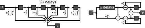
Since each half of the filter is a power series, they may be implemented recursively, as shown in the right hand panel of Figure 9.21. The bottom accumulator sums the terms in the first half of the window and needs to be 2k bits wide to avoid round-off errors. The upper accumulator sums the terms in the second half of the window. It does not need to subtract out the remainder after a further k delays, because that decays to zero (this is using an infinite impulse response filter).
The kernel for the 2-5-2 spline is:
(9.25) 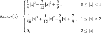
with the corresponding filter weights given as (Ferrari et al., 1999):
(9.26) 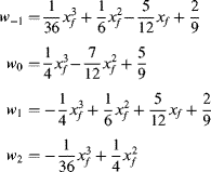
These are used in the same way as for the bicubic interpolation, although the awkwardness of these coefficients makes lookup table implementation better suited than direct calculation.
The filters given here are one dimensional. For two-dimensional filtering, the two filters can be used separably on the rows and columns, replacing the delays with row buffers. If the input is coming from a frame buffer, and the memory bandwidth allows, then the k row buffer delay may be replaced by a second access to the frame buffer in a similar manner to the box filter shown in Figure 8.20.
An FPGA implementation of this cubic spline filter was used to zoom an image by an integer factor by Hudson et al. (1998). The prefilter shown in the left of Figure 9.21 was used. The interpolation stage was simplified by exploiting the fact that a pure zoom results in a regular access pattern. Since this was fairly early work, the whole algorithm did not fit on a single FPGA. One-dimensional filters were implemented, with the data fed through separately for the horizontal and vertical filters. Dynamic reconfiguration was also used to separate the prefiltering and interpolation stages.
A wide range of other interpolation kernels is available; a review of the more commonly used kernels for image processing is given elsewhere (Wolberg, 1990). Very few of these have been used for FPGA implementation because of their higher computational complexity than those described in this section.
9.3.4 Interpolating Compressed Data
Interpolation can also be used to reduce the data volume when using non-parametric methods of representing geometric distortion, uneven illumination or vignetting. Rather than representing the map (either geometric transformation or intensity map) by a parametric model, the map is stored explicitly for each pixel. For a geometric transformation, this map represents the source location (for a reverse mapping) for each pixel in the output image (Wang et al., 2005). For modelling uneven illumination, the map contains the illumination level or correction scale factor directly for each pixel. This has two advantages over model-based approaches. Firstly, evaluating the map is simply a table lookup, so is generally much faster than evaluating a complex parametric model. Secondly, a non-parametric map is able to capture distortions and variations that are difficult or impossible to model with a simple parametric model (Bailey et al., 2005). However, these advantages come at the cost of the large memory required to represent the map for every pixel. If the map is smooth and slowly varying, then it can readily be compressed. The simplest form of compression from a computational point of view is to down-sample the map and use interpolation to reconstruct the map for a desired pixel (Akeila and Morris, 2008).
The resolution required to represent the down-sampled map obviously depends on the smoothness of the map, and also the accuracy with which it needs to be recreated. There is a trade-off here. Simple bilinear interpolation will require more samples to represent the map to a given degree of accuracy than a bicubic or spline interpolation requires, but require less computational logic to evaluate the map for a given location.
For stream processing, the required points will be aligned with the scan axis, simplifying the access pattern. The relatively small number of weights used can be stored in small RAMs (fabric RAM is ideal for this). With a separable mapping, the vertical mapping can be performed first, since each set of vertical points will be reused for several row calculations.
With stream processing, the input to the mapping function is a raster scan, regardless of whether a forward or reverse mapping is used (refer to Figure 9.2 to see that this is so). Therefore, incremental calculation can be used to simplify the computation by exploiting the fact that the y (or v) address is constant and the x (or u) address increments with successive pixels.
For an affine transformation, Equation 9.6 can be represented in matrix form as:
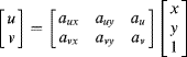
Implemented directly, this transformation would require six multiplications and four additions. With incremental calculation, the only change moving from one pixel to the next along a row is ![]() . Substituting this into Equation 9.27 gives:
. Substituting this into Equation 9.27 gives:
(9.28) 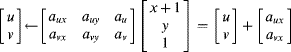
requiring only two additions. A similar simplification can be used for moving on to the next row. When implementing these, it is convenient to have a temporary register to hold the position at the start of the row. This may be incremented when moving from one row to the next and is used to initialise the main register, which is updated for stepping along the rows, as shown in Figure 9.22. It is necessary that these registers maintain sufficient guard bits to prevent the accumulation of round-off errors.
Figure 9.22 Incremental mapping for affine transformation.
Equation 9.27 can be extended to a perspective transformation using homogenous coordinates:
(9.29) 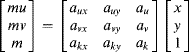
where the third row gives a position dependent magnification, m. The mu and mv terms are then divided by m to give the transformed coordinates. The same incremental architecture from Figure 9.22 may be used for the perspective transformation, with the addition of a division at each clock cycle to perform the magnification scaling.
The mappings shown here for the affine and perspective transformations are for forward mappings. The reverse mappings will have the same form and may be determined simply by inverting the corresponding transformations.
Using incremental mapping for polynomial warping is a little more complex. Consider just the u component of a second order polynomial forward mapping:
(9.30) ![]()
First consider the initialisation of each row:
(9.31) ![]()
For the row increment, it is necessary to know the value from the previous row:
(9.32) ![]()
Therefore:
(9.33) ![]()
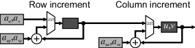
with the second term produced by another accumulator, as shown in Figure 9.23.
Figure 9.23 Incremental calculation for a second order polynomial warp.
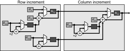
For the column increment along the row, it is necessary to know the previous value:
(9.34) ![]()
Therefore:
(9.35) ![]()
where the second term is produced by a secondary accumulator incremented with each column and the third term is provided by a secondary accumulator incremented each row.
A parallel circuit is also required for the v component. A similar approach may be taken for higher order polynomial mappings, with additional layers of accumulators required for the higher order terms.
Unlike the affine and perspective mappings, the inverse of a polynomial mapping is not another polynomial mapping. Therefore, it is important to determine the mapping coefficients for the form that is being used. It is not a simple matter to convert between the forward and reverse mapping.
In the previous sections, it was assumed that the geometric transformation was known. Image registration is the process of determining the relationship between the pixels within two images, or between parts of images. There is a wide variety of image registration methods (Brown, 1992; Zitova and Flusser, 2003), of which only a selection of the main approaches are outlined here. General image registration involves four steps (Zitova and Flusser, 2003): feature detection, feature matching, transform model estimation and image transformation and resampling. The last step has been discussed in some detail earlier in this chapter. This section will therefore focus on the other steps. There are two broad classes of registration: those based on matching sets of feature points and those based on matching extended areas within the image. Since these are quite different in their approach, they are described separately. This section concludes with some of the applications of image registration.
9.5.1 Feature-Based Methods
A common approach to registration is to find corresponding points within the images to be registered. While such points can be found manually, this precludes automatic processing. Therefore, a feature extraction step is required that locates salient and distinctive points within each image. Ideally, these should be well distributed throughout the image and be easy to detect. The features should also be invariant to the expected transformation between the images. Once a set of features is found, it is then necessary to match these between images. Not all feature points found in one image may be found in the other, so the matching method must be robust against this.
9.5.1.1 Feature Detection
If the scene is contrived (as is often the case when performing calibration), for example consisting of a array of dots, a checkerboard pattern or a grid, then the detection method can be tailored specifically to those expected features. For an array of dots, adaptive thresholding can reliably segment the dots, with the centre of gravity used to define the feature point location. With a checkerboard pattern, either an edge detector is used to detect the edges, from which the corners are inferred, or a corner detector is used directly. A corner detector is just a particular filter that is tuned to locating corners (Noble, 1988). Consequently, corner detectors can be readily implemented on FPGAs (Claus et al., 2009). For grid targets, a line detector can be used, with the location of the intersections identified as the feature point locations. An example of this is considered in more detail in Section 14.2.
The regular structure of a contrived target makes correspondence matching relatively easy because the structure is known in advance. The danger with using a periodic pattern is that the matched locations may be offset by one or more periods between images. This may be overcome by adding a distinctive feature within the image that can act as a key for alignment.
Edge and corner features can also be used with natural scenes, but often do not work as well because such points are usually not as well defined in terms of contrast, and there may be many features detected in one image but not the other. To overcome this, it is necessary to find only the dominant features which are likely to appear in both images. While there are several approaches that could be taken, one that has gained prominence in recent years is the scale invariant feature transform (SIFT).
SIFT (Lowe,1999; 2004) filters the images with a series of Gaussian filters to obtain a representation of the image at a range of scales. The difference between successive scales (a difference of Gaussian filter) is a form of band-pass filter that responds most strongly to objects or features of that scale. The local maxima and minima within each scale are then located and compared with adjacent scales, both larger and smaller. The local extremes both spatially and in scale that are greater than a preset threshold (3% of the pixel range), are considered as possible feature points and are located to subpixel accuracy. Since the difference of Gaussian filter also responds strongly to edges, there is a danger that a point will be poorly located along the edge and, therefore, be sensitive to small amounts of noise. Therefore, it is necessary to eliminate peaks which are poorly defined along the edge direction. Let D be the response of the difference of Gaussian filter. Then only the points which satisfy
(9.36) ![]()
are kept, where ![]() ,
, ![]() and
and ![]() are second derivatives and the threshold
are second derivatives and the threshold ![]() (Lowe, 2004).
(Lowe, 2004).
The feature orientation is determined by taking the derivatives of the Gaussian filtered image at the appropriate scale. The orientations within a window are examined and the dominant direction determined through weighted averaging. Finally, local gradient information is used to derive a descriptor of the feature point. The feature orientation is used as the reference to give orientation independence, with the descriptor built from a set of histograms of gradients weighted by edge strength. Basing the descriptor on gradients reduces the sensitivity to absolute light levels, and normalising the final feature to unit length reduces sensitivity to contrast, improving the robustness.
In implementing a feature detection algorithm such as SIFT, most of the computation is spent in filtering image. Typically less than 1% of the pixels within the image are feature points. Several factors can be exploited to filter the images efficiently. The first is that the Gaussian window is separable, so the two-dimensional filter can be decomposed into a one-dimensional filter along the rows and a one-dimensional filter down the columns. Secondly, a Gaussian of a larger scale may be formed by cascading another Gaussian filter over the already processed image. Thirdly, after blurring the image sufficiently, it may be safely down-sampled, reducing the volume of processing in the subsequent stages. These stages are illustrated in Figure 9.24. Each of the blocks (apart from the feature point processing) was a filter described in Chapter 8, and the feature processing is outlined above.
Figure 9.24 SIFT feature point extraction.
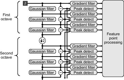
Such processing has been implemented on an FPGA. Pettersson and Petersson (2005) used five element Gaussian filters and four iterations of CORDIC to calculate the magnitude and direction of the gradient. They also simplified the gradient calculation, with only one filter used per octave rather than one per scale. Chang and Hernandez-Palancar (2009) made the observation that after down-sampling the data volume is reduced by a factor of four. This allows all of the processing for the second octave and below to share a single Gaussian filter block and peak detect block.
Yao et al. (2009) took the processing one step further and also implemented the descriptor extraction in hardware. The gradient magnitude used the simplified formulation of Equation 8.18 rather than the square root, and a small lookup table was used to calculate the orientation. They used a modified descriptor that had fewer parameters, but was easier to implement in hardware. The feature matching, however, was performed in software using an embedded MicroBlaze processor.
9.5.1.2 Feature Matching
The matching step aims to find the correspondence between features detected in the two images. Again, there is a wide range of matching techniques (Zitova and Flusser, 2003), with a full description beyond the scope of this work. The method based on invariant descriptors used by SIFT will be discussed as an example of one matching algorithm.
Features descriptors which are invariant to the expected transformation may be matched by finding the feature in the reference image which has the most similar descriptor. The descriptor match is unlikely to be exact because of noise and differences resulting from local distortions. With a large number of descriptors and a large number of components within each descriptor, a brute force search for the closest match is prohibitive. Therefore, efficient search techniques are required to reduce the search cost.
If the reference is within a database, for example when searching for predefined objects within an image, then two approaches to reduce the search are hashing and tree-based methods. A locality sensitive hash function (Gionis et al., 1999) compresses the dimensionality, enabling approximate closest points to be found efficiently. Alternatively, the points within the database may be encoded in a high-dimensional tree-based structure and, using a best bin first heuristic, the tree may be searched efficiently (Beis and Lowe, 1997). Such searches for a particular point are generally sequential. While the search for multiple points may be performed independently, implying that they may be searched in parallel, for large databases this is also impractical. Serial search methods with complex data structures and heuristics may be best performed in software, although it may be possible to accelerate key steps using appropriate hardware.
For matching between images, one approach is to build a database of points from the reference image and use the approaches described in the previous paragraph. An alternative is to combine the matching and model extraction steps. The first few points are matched using a full search. These are then used to create a model of the transformation, which is used to guide the search for correspondences for the remaining points. New matches can then be used to refine the transformation. Again, the search process is largely sequential, although hardware may be used to accelerate the transformation to speed up the search for new matches.
9.5.1.3 Model Extraction
Given a set of points, the transformation model defines the best mapping of the points from one image to the other. For a given model, determining the transformation can be considered as an optimisation problem, where the model parameters are optimised to find the best match.
If the model is sufficiently simple (for example an affine model, which is linear in the model parameters) it may be solved directly using least squares minimisation. Consider for example the affine mapping of Equation 9.6; this may be represented in matrix form in terms of the transform coefficients (compare this with Equation 9.27) as:
(9.37) 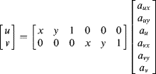
Each pair of corresponding points provides two constraints. Therefore, the set of equations for N sets of control points has 2N constraints:
(9.38) 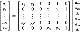
or
(9.39) ![]()
Usually this set of equations is over-determined and with noise it is impossible to find model parameters which exactly match the constraints. In this case, the transform parameters can be chosen such that the total squared error is minimised:
(9.40) ![]()
This is minimised by taking the partial derivative with respect to each parameter and setting the result to zero:
(9.41) ![]()
so solving
(9.42) ![]()
to give
(9.43) ![]()
yields the least squares solution. The regular nature of matrix operations and inversion makes them amenable to FPGA implementation (Irturk et al., 2008; Burdeniuk et al., 2010), although if care is not taken with scaling this can result in significant quantisation errors if fixed-point arithmetic is used. Least squares optimisation is quite sensitive to outliers, so robust fitting methods can be used, if necessary, to identify outliers, and remove their contribution from the solution.
If the corresponding points may come from one of several models, then the mixture can cause even robust fitting methods to fail. One approach suggested by Lowe (2004) was to have each pair of corresponding points vote for candidate model parameters using a coarse Hough transform (the principles of the Hough transform are described in Section 11.7). This effectively sorts the pairs of corresponding points based on the particular model, filtering the outliers from each set of points.
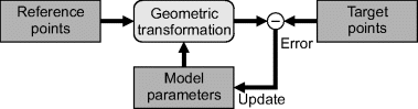
With more complex or nonlinear models, a closed form solution of the parameters is not possible. In this case, it is common to use an iterative technique as outlined in Figure 9.25. An initial estimate of the model is used to transform the reference points. The error can then directly be measured against the target points, with the error used to update the model using steepest descent or Levenberg–Marquardt (Press et al., 1993) error minimisation.
Figure 9.25 Iterative update of registration model.
9.5.2 Area-Based Methods
The alternative to feature-based image registration is to match the images themselves, without explicitly detecting objects within the image. Such area matching may be performed on the image as whole, or on small patches extracted from the image.
Area-based matching has a number of limitations compared with feature-based matching (Zitova and Flusser, 2003). Any distortions within the image affect the shape and size of objects within the image and, consequently, the quality of the match. Similarly, since area matching is generally based on matching pixel values, the matching process can be confounded by any change between the images, for example by varying illumination or using different sensors. When using small image patches, if the patch is textureless without any significant features, it can be matched with just about any other smooth area within the other image, and often the matching is based more on noise or changes in shading rather than a true match. In spite of these limitations, area-based matching is in common use.
9.5.2.1 Correlation Methods
The classical area matching method is cross-correlation. This extends Equation 6.40 by removing the mean from the two images:
(9.44) 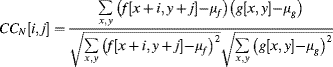
Although, for computational simplicity, the simple sum of absolute differences (Equation 6.24) or sum of squared differences (Equation 6.25) is often substituted for the correlation as a measure of similarity. The offset that gives the maximum correlation or minimum difference provides the best registration. When looking for a smaller target within a larger image, this process is often called template matching. If the target is sufficiently small, this can be implemented directly using filtering to produce an image of match scores, where the local maxima above a threshold (or minima for difference methods) are the detected locations of the target.
There are several limitations with correlation for image matching. It is generally restricted to a simple translational model, although for correlating small patches it can tolerate small image imperfections. It is also computationally expensive, especially when matching one image to another. While measuring the similarity is straightforward, it is necessary to repeat this measurement over all possible offsets to find the maximum. Since the correlation surface is usually not of particular interest, the computation may be reduced by restricting the number of different offsets that are measured. Such techniques use search methods to find the optimum offset. This is complicated, however, by the fact that there may be several local maxima so there is a danger of finding the wrong offset.
One technique commonly used to reduce the search complexity is to use a pyramidal approach to the search. An image pyramid is produced by filtering and down-sampling the images to produce a series of progressively lower resolution versions. These enable a wide range of offsets to be searched relatively quickly for two reasons: the lower resolution images are significantly smaller, so measuring the similarity for each offset is faster, and a large step size is used because each pixel is much larger. This enables the global maximum to be found efficiently, even using an exhaustive search at the lowest resolution if necessary. The estimated offset obtained from the low resolution images may not be particularly accurate, but can be refined by finding the maximum at progressively higher resolutions. These latter searches are made more efficient by restricting the search region to the global maximum and can safely perform restricted searches without worry of locking onto the wrong peak.
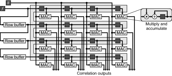
It is straightforward to perform the correlation for multiple offsets in parallel. One way of achieving this is shown in Figure 9.26, where the 16 correlations within a 4 × 4 search window are performed in parallel in a single scan through the pair of images. One of the input images is offset relative to the other by a series of shift registers and row buffers, with a multiply and accumulate (MAC) unit at each offset of interest. The multiplication could just as easily be replaced by an absolute difference or squared difference. With a pyramidal search, a block such as this can be reused for each level of the pyramid.
Figure 9.26 Calculating a 4 × 4 block of cross correlations in parallel.
The correlation peak is found to the nearest pixel. To estimate the offset to subpixel accuracy, it is necessary to interpolate between adjacent correlation values. Commonly a parabola is fitted between the maximum pixel, ![]() , and those on either side. The horizontal subpixel offset is then:
, and those on either side. The horizontal subpixel offset is then:
(9.45) ![]()
and similarly for the vertical offset (Tian and Huhns, 1986). However, fitting a pyramid has been found to be better (the autocorrelation of a piece-wise constant image has a pyramidal peak) (Bailey and Lill, 1999; Bailey, 2003). This gives the subpixel offset as:
(9.46) ![]()
Extending correlation-based matching to transformations more complex than simple translation quickly becomes computationally intractable. Each transformation parameter adds an additional dimension to the search space and effectively requires the image to be transformed for each iteration of the comparison.
9.5.2.2 Fourier Methods
Another approach to accelerating correlation is to perform the computation in the frequency domain. Consider unnormalised correlation:
Taking the two-dimensional discrete Fourier transform of Equation 9.47:
converts the correlation to a simple product in the frequency domain, where u and v are the spatial frequencies in the x and y directions respectively, and ![]() is the complex conjugate of F. Therefore, the computation to perform an exhaustive search may be significantly reduced by taking the Fourier transform of each image, calculating the product and then taking the inverse Fourier transform. (See Section 10.1 for implementing the Fourier transform on an FPGA.) The limitations of using a simple unnormalised correlation apply to using the Fourier transform to implement the correlation. It is not easy to incorporate normalisation without destroying the simplicity of Equation 9.48.
is the complex conjugate of F. Therefore, the computation to perform an exhaustive search may be significantly reduced by taking the Fourier transform of each image, calculating the product and then taking the inverse Fourier transform. (See Section 10.1 for implementing the Fourier transform on an FPGA.) The limitations of using a simple unnormalised correlation apply to using the Fourier transform to implement the correlation. It is not easy to incorporate normalisation without destroying the simplicity of Equation 9.48.
Phase correlation reduces this problem by considering only the phase. If f is the offset version of g:
(9.49) ![]()
then from the shift theorem of the Fourier transform (Bracewell, 2000), in the frequency domain this becomes:
(9.50) ![]()
Taking the phase angle of the ratio of the two spectra gives:
There are two methods by which the offset may be estimated. The first is to normalise the magnitudes to one and take the inverse Fourier transform:
(9.52) ![]()
where ![]() is a delta function at
is a delta function at ![]() . Phase noise, combined with the fact that the offset is not likely to be exactly an integer number of pixels, means that the output is not a delta function. However, a search of the output for the maximum value will usually give the offset to the nearest pixel.
. Phase noise, combined with the fact that the offset is not likely to be exactly an integer number of pixels, means that the output is not a delta function. However, a search of the output for the maximum value will usually give the offset to the nearest pixel.
The second approach is to fit a plane to the phase difference in Equation 9.51 using least squares. This first requires unwrapping the phase, because the arctangent reduces the phase to within ![]() . In practise, the quality of the phase estimate at a given frequency will depend on the amplitude. Therefore, the fit may be formed by weighting the phase samples by their amplitudes, or masking out those frequencies with low amplitude or those that differ significantly in amplitude between the two images (Stone et al., 1999; 2001).
. In practise, the quality of the phase estimate at a given frequency will depend on the amplitude. Therefore, the fit may be formed by weighting the phase samples by their amplitudes, or masking out those frequencies with low amplitude or those that differ significantly in amplitude between the two images (Stone et al., 1999; 2001).
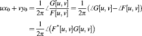
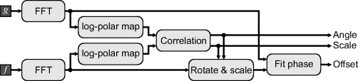
Just using the Fourier transform is limited to pure translation, although the offset may be estimated to subpixel accuracy. To extend the registration to include rotation and scaling requires additional processing. Rotating an image will rotate its Fourier transform and scaling an image will result in an inverse scale within the Fourier transform. Therefore, by converting the Fourier transform from rectangular coordinates to log-polar coordinates (the radial axis is the logarithm of the frequency), rotating the image corresponds to an angular shift and scaling the image results in a radial shift (Reddy and Chatterji, 1996). The angle and scale factor may be found by correlation (or even using a Fourier-based method to estimate the offset. The structure of the algorithm is shown in Figure 9.27.
Figure 9.27 Fourier-based registration, including a rotation and scale factor.
9.5.2.3 Gradient Methods
Rather than perform an exhaustive search in correlation space, gradient-based methods effectively perform a hill climbing search using an estimate of the offset based on derivatives of the image gradient. Expanding an offset image, ![]() , about
, about ![]() using a two-dimensional Taylor series gives:
using a two-dimensional Taylor series gives:
(9.53) ![]()
For small offsets, the Taylor series can be truncated (the second order and higher terms are considered negligible and contribute to noise). Therefore, given estimates of the gradients, the offset may be estimated from:
(9.54) ![]()
where the gradients may be obtained from a central difference filter. Each pixel then provides a constraint; since this over-determined system is linear in the offsets ![]() and
and ![]() , it may be solved by least squares minimisation (Lucas and Kanade, 1981).
, it may be solved by least squares minimisation (Lucas and Kanade, 1981).
(9.55) 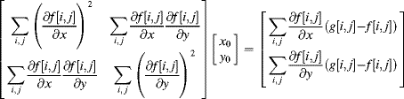
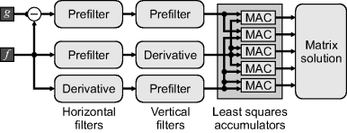
The Taylor series approximation may be improved by prefiltering the images with a low pass filter. The derivatives can then be obtained by using a matching the derivative filter to the derivative of the prefilter (Farid and Simoncelli, 2004). The optimal low order filter pairs are listed in Table 9.1. In two dimensions, the filters are separable, resulting in a pipelined implementation similar to Figure 9.28.
Table 9.1 Filter coefficients for optimal prefilters and derivative filters. (Reproduced with permission from H. Farid and E.P. Simoncelli, “Differentiation of discrete multidimensional signals,” IEEE Transactions on Image Processing, 13, 4, 496–508, 2004. © 2004 IEEE.)
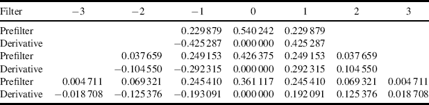
Figure 9.28 Basic approach of gradient-based registration.
Since the offset is only approximate (it neglects the high order series expansion terms) the expansion may be repeated about the approximation. After the first approximation, the offset will be closer, so the truncated Taylor series will be more accurate, enabling a more accurate estimate of the offset to be obtained. Iterating the formulation will converge to the minimum error (Lucas and Kanade, 1981).
Variations on this theme can manage more complex geometric transformations or use different optimisation techniques to minimise the error (Baker and Matthews, 2004). More complex transformations follow the general iterative pattern of Figure 9.25. These, too, can be based on a pyramidal coarse-to-fine search strategy to reduce the chances of becoming locked onto a local minimum (Thevenaz et al., 1998). The initial match is based on large scale features, with the successive refinements at finer scales making small corrections for finer details.
Registration is also used to combine data from difference sensor types. This is common in both remote sensing and medical imaging. The basic image matching metrics of correlation or sum of absolute differences do not perform very well at registering images where there are significant differences in contrast. In these instances, is more effective to find the transformation that maximises mutual information (Viola and Wells, 1997).
9.5.2.4 Optimal Filtering
When looking at subpixel registration involving pure translation, the gradient-based methods effectively create a continuous surface through interpolation, which is then resampled with the desired offset. This is then compared with the target image, as in Figure 9.25, to minimise the error. Expressing the interpolation as a convolution in the form of Equation 9.15 gives:
(9.56) ![]()
where ![]() is the interpolation kernel for an offset of
is the interpolation kernel for an offset of ![]() . Finding the offset that minimises this error requires a search because the filter coefficients, and hence the relationship between the two images, depends nonlinearly on the offset.
. Finding the offset that minimises this error requires a search because the filter coefficients, and hence the relationship between the two images, depends nonlinearly on the offset.
Predictive interpolation (Bailey and Lill, 1999) avoids the search by turning the problem around. Rather than use an interpolation kernel that makes arbitrary assumptions about the image (such as being band-limited or smooth), the optimal interpolation kernel is derived by predicting the pixel values of the target image from the reference (Bailey and Gilman, 2007; Gilman and Bailey, 2007). This solves:
where the subtraction of ![]() enforces the partition of unity constraint (Unser, 2000)
enforces the partition of unity constraint (Unser, 2000)
(9.58) ![]()
Since Equation 9.57 is linear in the filter coefficients, it may be solved by least squares. Representing Equation 9.57 in matrix form:
(9.59) ![]()
where ![]() are the filter coefficients arranged as a vector, and each line in
are the filter coefficients arranged as a vector, and each line in ![]() and
and ![]() corresponds to one pixel in the image. The least squares solution becomes:
corresponds to one pixel in the image. The least squares solution becomes:
(9.60) ![]()
Then, given the optimal interpolation filter, the problem becomes one of estimating the offset from the filter coefficients. This may be obtained from a weighted sum of the filter coefficients (Bailey and Gilman, 2007; Gilman and Bailey, 2007) with the weights dependent only on the coefficient index:
(9.61) ![]()
or
(9.62) ![]()
where ![]() is the matrix of constant weights. Predictive interpolation therefore gives a direct (non-iterative) solution to estimating the offset between images to subpixel accuracy.
is the matrix of constant weights. Predictive interpolation therefore gives a direct (non-iterative) solution to estimating the offset between images to subpixel accuracy.
The cost of this approach is as follows: assume that the prediction window is ![]() pixels, requiring
pixels, requiring ![]() filter coefficients to be calculated (
filter coefficients to be calculated (![]() is not required).
is not required). ![]() requires
requires ![]() MACs and
MACs and ![]() requires
requires ![]() (because of symmetry). This grows very quickly with window size, especially as windows with odd
(because of symmetry). This grows very quickly with window size, especially as windows with odd ![]() do not perform as well (Bailey and Gilman, 2007). While only nine MAC units are required in total for a 2 × 2 window (Figure 9.29), this grows to 135 for 4 × 4, and 665 for 6 × 6. Most of the hardware is required for building
do not perform as well (Bailey and Gilman, 2007). While only nine MAC units are required in total for a 2 × 2 window (Figure 9.29), this grows to 135 for 4 × 4, and 665 for 6 × 6. Most of the hardware is required for building ![]() . To reduce the hardware, it is necessary to reduce the pixel clock and share the MACs. However, when registering multiple images,
. To reduce the hardware, it is necessary to reduce the pixel clock and share the MACs. However, when registering multiple images, ![]() and its inverse only need to be calculated once.
and its inverse only need to be calculated once.
Figure 9.29 Predictive interpolation with a 2 × 2 window.
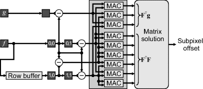
While optimal filtering provides the offset to subpixel accuracy, the images must already be registered to the nearest pixel (this can be relaxed slightly with larger windows). Again, a pyramidal coarse-to-fine search or other registration methods may be used to give the initial approximation. The optimal filtering approach is restricted to translation only, and cannot easily be extended to include more general transformations.
9.5.3 Applications
There are many applications of image registration or related techniques. The applications are quite diverse, with variations on some of the techniques described above used to address issues unique to that application. While it is not possible to describe all of the applications in any detail, a brief overview of some of the main applications is given.
Perhaps the most common is camera calibration, where it is desired to determine the geometric transformation which describes the imaging model of the camera, including its pose. To define the mapping between points within the real world, and pixels within the image, it is usually necessary to have a target object with distinctive features in known physical locations. This simplifies feature detection and the process becomes one of determining the camera model. Examples of a range of different models and methods of solving them are given elsewhere (Brown, 1971; Tsai, 1987; Heikkila and Silven, 1997; Devernay and Faugeras, 2001; Kannala and Brandt, 2004).
Image and video compression rely on reducing the redundancy inherent within an image or image sequence. When encoding a video sequence, there is significant correlation from one frame to the next that can be exploited to reduce the data volume. Therefore, rather than encode each image independently, considerable compression may be obtained by encoding the difference between the current and previous frame. This works well with static objects, but any motion creates a misalignment, reducing the gains. To achieve good compression, it is necessary to compensate for such motion. This is most commonly achieved by dividing the current frame into small blocks (typically 8 × 8 or 16 × 16) and finding the best offset between each block and the corresponding data in the previous frame. FPGAs have been the target for performing the matching at a rate that enables real-time compression. For example, Wong et al. (2002) developed a system that could perform the sum of absolute differences of a row or column of pixels in parallel. For each pair of pixels, this determined which of the corresponding pixels was smaller, so it could be inverted before being passed into an adder. All of the pixels were added, along with a correction term to convert one's complement to two's complement, by a single large adder tree. To reduce propagation delay, carry save adders were used, configured as a 33 to 2 reduction, followed by a final addition. To accelerate finding the best matched block, Dubois et al. (2005) built a system that could perform a random search with programmable block size. Yu et al. (2004) used a restricted two-step search to reduce the search space by a factor of 15 over a full search, enabling a reduced number of processing elements to be used.
Optical flow involves the estimation of motion fields within an image. This generally requires matching small patches from one frame with the previous frame. In this way it is similar to motion compensation for video coding. The difference is that with optical flow it is desired to have a coherent flow field, rather than treat each patch independently. FPGA implementations of optical flow have been reported by Diaz et al. (2004) and Wei et al. (2008).
Stereo imaging processes separate images from two spatially separated cameras to extract the disparity or differences in relative position of objects between the two images. The disparity is dependent on the range to the object of interest, enabling range data to be extracted. One of the motivating applications is the real-time extraction of range data for driver assistance and collision avoidance. The search for matches may be simplified with stereo imaging by exploiting epipolar geometry. An object point, when combined with the two camera centres, defines a plane in three-dimensional space. All points on that plane will be imaged to a single line in each of the captured images. Therefore, the search for corresponding points may be restricted to a one-dimensional search along these epipolar lines. This search process may be simplified by first rectifying the images to map the epipolar lines onto the image scanlines.
A wide range of stereo matching algorithms can be used – here is a sampling of recent papers which describe an FPGA implementation. Masrani and MacLean (2006) used correlation, with a multiresolution search centred on the disparity detected in the previous frame, working on the assumption that the disparity should not change significantly in one frame period. Longfield and Chang (2009) used a census transform to reduce the cost of finding a match. The census transform thresholds a local window with the central value, giving a binary template which may be matched more easily. Rather than find a local match, Morris et al. (2009) used dynamic programming to find a consistent set of matches across the whole row. Each potential match has a penalty given by the absolute difference in pixel values, with additional penalty for occlusion (a point visible in only one of the images).
Image super-resolution combines several low resolution images of a scene to create a single image with higher spatial resolution. Super-resolution reconstruction typically requires three steps: registration of the input images to subpixel accuracy; resampling the ensemble at the higher resolution; and inverse filtering to reduce the blur resulting from the low resolution imaging process. Again, there is a wide range of techniques used for image super-resolution. Many are iterative and not amenable to real-time implementation, although the algorithms may be accelerated using an FPGA as the computation engine. The optimal filtering techniques have potential, not only for image registration, but also for determining efficient resampling (interpolation) filters (Gilman, 2009; Gilman et al., 2010). Little has been implemented so far on FPGAs. Perhaps one exception is the work of Bowen and Bouganis (2008), although their work assumed that the images were already registered and only considered the image combination stage.