
Chapter 7
Histogram Operations
As indicated in the previous chapter, the parameters for many point operations can be derived from the histogram of pixel values of the image. This chapter is divided into to two parts: the first considers greyscale histograms and some of their applications, and the second extends this to multidimensional histograms.
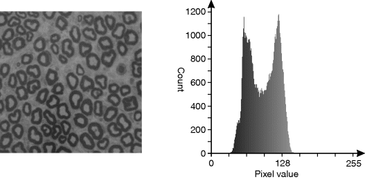
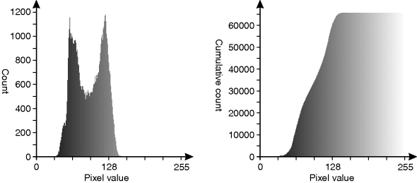
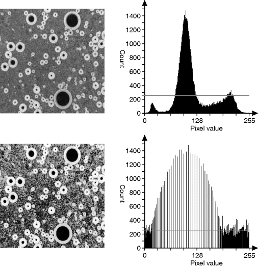
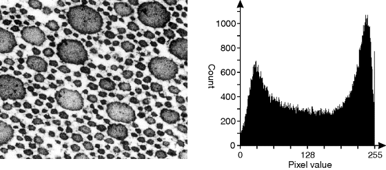
The histogram of a greyscale image, as shown in Figure 7.1, gives a count of the number of pixels in an image as a function of pixel value.
Figure 7.1 An image and its histogram.
There are two main steps associated with using histograms for image processing. The first step is to build the histogram, and the second is to extract data from the histogram and use it for processing the image. Building the histogram is discussed in this section, whereas the applications are described in subsequent sections.
To build the histogram, it is necessary to accumulate the counts for each pixel value, as indicated in Equation 7.1. Since each pixel must be visited once, building the histogram is ideally suited to stream processing. To accumulate the pixel count for each pixel value requires maintaining the count so far for each value. This may be accomplished by an array of counters, with the input pixel used to enable the clock of the corresponding counter (Figure 7.2). The output counts need to be indexed using a bus or multiplexer.
Figure 7.2 Histogram accumulator built from counters.
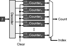
A disadvantage of this approach is that the decoding and output multiplexing are relatively expensive. The decoder of the input pixel stream may be re-used as part of the output multiplexer; however, the number of different pixel values (or histogram bins) means that a large amount of logic cannot be avoided. The counters and associated registers must also be built using the logic resources of the FPGA, with each counter register built from flip-flops. This approach is, therefore, best suited if only a few counters are required (for example after thresholding), or if processing requires the individual counters to be accessed in parallel.
Each pixel can have only one pixel value, so only one counter is incremented in any clock cycle. This implies that the accumulators may be implemented in memory. Incrementing an accumulator requires reading the associated memory location, adding one, and writing the sum back to memory. This requires a dual-port memory, with one port being used to read the memory and one port to write the result. This scheme is shown in Figure 7.3. Memory is effectively a multiplexed register bank. However, from an implementation perspective, the multiplexers are built within the memory addressing, so significantly fewer logic resources are required.
Figure 7.3 Histogram accumulation using dual-port memory.
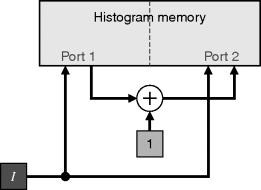
One disadvantage of the memory-based approach is that resetting the registers at the start of a frame requires sequentially cycling through memory locations to set them to zero. With the register-based approach of Figure 7.2, all of the registers may be reset in parallel.
The circuit of Figure 7.3 requires a late write to the second port. This requires the timing to allow the data to be read near the start of the clock cycle, so the incremented value may be written at the end of the clock cycle. This may be readily achieved with asynchronous memory or by delaying the write pulse for synchronous memory.
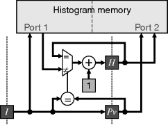
If a late write is not available, then both the pixel value and the accumulated count must be buffered in registers to enable the updated count to be written in the following clock cycle. It is slightly more complicated than this, as shown in Figure 7.4, because if the subsequent pixel has the same value, the count read from memory will not have been updated yet. This requires checking if the current pixel is the same as the previous value, and if so incrementing the registered value rather than that read from memory.
Figure 7.4 Performing histogram accumulation with caching when late write is not available.
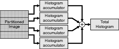
As each pixel is processed independently, it is also possible to partition the image over several parallel accumulators (Figure 7.5). This approach then requires a final pass through the accumulators to combine the results from each partition to give the histogram for the complete image.
Figure 7.5 Partitioning the accumulation over several parallel processors.
The circuitry that processes the histogram to extract data from it must operate on the same histogram. Similarly, the circuitry that resets the histogram must also be connected to the histogram memory. These require multiplexing the address and data lines to the appropriate data structures. These multiplexers are assumed in the following sections.
7.1.1 Data Gathering
Histograms may be used to gather data from the objects within the image. Consider an image of a single object, and that object can be separated from the background by thresholding. Then the area of the object is simply given by the number of pixels detected by thresholding. This may be obtained from the histogram of the corresponding binary image. Obviously, it is unnecessary to build a complete histogram for this case, a single counter will suffice (compare with Figure 7.2). However, if the threshold level is obtained by processing the histogram, then the area may be found directly from the histogram without necessarily thresholding the input image:
(7.2) ![]()
This idea may be generalised to measuring the area of many objects within an image. If the image is processed in such a way that the pixels associated with each object within the image are assigned a unique label, then each histogram bin will be associated with a different label, effectively giving the area of each object.
Other useful statistics of the image, such as the mean and variance, may be extracted from the histogram, rather than directly from the image. While these may be calculated directly from the image, if the statistics are taken from a restricted range of pixel values that is chosen dynamically, it is more efficient to obtain the histogram as an intermediate step.
The mean pixel value of an image is given by:
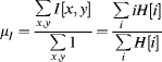
with the variance as:
The last form of Equation 7.4 allows the variance to be calculated in parallel with the mean, rather than having to calculate the mean first. Often, the mean and variance within a restricted range of pixel values is required rather than over the full range. In this case, the summations of Equations 7.3 and 7.4 are performed over that range (![]() to
to ![]() ).
).
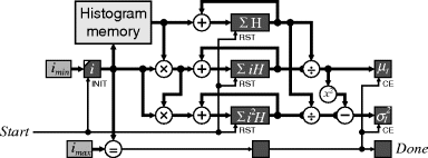
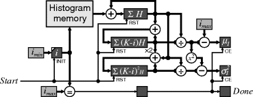
A direct implementation of these summations is shown in Figure 7.6. The start signal selects ![]() into i and resets the summations to zero. On subsequent clock cycles, H[i] is read and added to the appropriate accumulators. If the delay through the multiplications is too long, then this may be pipelined. When i reaches
into i and resets the summations to zero. On subsequent clock cycles, H[i] is read and added to the appropriate accumulators. If the delay through the multiplications is too long, then this may be pipelined. When i reaches ![]() , the final summation is performed and the divisions to calculate the mean and variance carried out. Again, if the divisions take too long, they may be pipelined. The Done output goes high to indicate the completion of the calculation.
, the final summation is performed and the divisions to calculate the mean and variance carried out. Again, if the divisions take too long, they may be pipelined. The Done output goes high to indicate the completion of the calculation.
Figure 7.6 Calculating the mean and variance from a range of values within the histogram.
While the divisions on the output cannot easily be avoided, it is possible to share the hardware for a single division between the two calculations. The division can also be pipelined if necessary. If the standard deviation is required (rather than the variance) then a square root operation must be applied to the variance output. This may be accomplished with less logic than the division (Li and Chu, 1996).
The multiplications associated with the summations may be eliminated by using incremental update. Firstly, consider the summation, where K is an arbitrary constant:
Therefore:
(7.6) ![]()
Similarly:
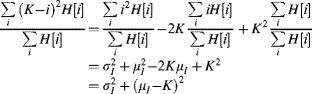
Therefore:
(7.8) 
Next, consider the incremental calculation of Equations 7.5 and 7.7:
(7.9) 
From
(7.10) ![]()
Therefore, starting K with ![]() and incrementing until
and incrementing until ![]() allows the summations to be performed without any multiplications (the factor of two in Equation 7.11 is simply implemented with a left shift). The resulting circuit is shown in Figure 7.7.
allows the summations to be performed without any multiplications (the factor of two in Equation 7.11 is simply implemented with a left shift). The resulting circuit is shown in Figure 7.7.
Figure 7.7 Using incremental calculations for the mean and variance.
The circuits of Figures 7.6 and 7.7 are fine if only a single calculation is required. However, if the mean and variance are required for several different ranges, then the repeated summation can become a time bottleneck. If timing becomes a problem, then this may be overcome by building sum tables that contain cumulative moments of the histogram:
(7.12) 
The first, ![]() , is also called the cumulative histogram, an example of which is shown in Figure 7.8. These tables require a single pass through the histogram to construct and, after that, the mean and variance of any range may be calculated with two accesses to each table:
, is also called the cumulative histogram, an example of which is shown in Figure 7.8. These tables require a single pass through the histogram to construct and, after that, the mean and variance of any range may be calculated with two accesses to each table:
Figure 7.8 Left: a histogram; right: its cumulative histogram.
Higher order moments (skew and kurtosis) may also be calculated in a similar manner by extension of the above circuit.
The statistical range of pixel values within an image is probably best calculated directly from the image as it is streamed. However, if the histogram is already available for other processing then it is a simple manner to extract the range from the histogram. The minimum pixel value, ![]() , is the smallest index that has a non-zero count, and the maximum pixel value,
, is the smallest index that has a non-zero count, and the maximum pixel value, ![]() , is the largest. A common operation using the range is contrast expansion using Equation 6.2 with:
, is the largest. A common operation using the range is contrast expansion using Equation 6.2 with:
(7.14) ![]()
Calculating the median of an image is probably easiest using the cumulative histogram of the image. The image median is defined as the bin that contains the fiftieth percentile. Ideally, an inverse cumulative histogram could be used; this maps from the cumulative count back to the corresponding pixel value. However, this can be derived from the cumulative histogram:
where ![]() is the number of pixels in the image and:
is the number of pixels in the image and:
(7.16) ![]()
Rather than scan through the histogram to find the median, Equation 7.15 may be solved with a binary search, with each successive iteration giving one bit of the median.
The image median may be generalised to determine the median value within a range of pixel values:
(7.17) ![]()
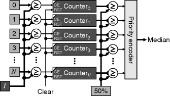
The architecture of Figure 7.2 may be adapted to build the cumulative histogram directly (Fahmy et al., 2005). Figure 7.9 demonstrates how this works. The decoder enables the clock of all of the counters greater than or equal to the pixel value, causing them to be incremented. After the whole image has been accumulated, the counters represent the cumulative histogram. As the outputs of all these counters are available, they can be compared with the median count (indicated by ‘50%’ in the figure) in parallel. The priority encoder finds the minimum output that has a one, as required by Equation 7.15, and returns the corresponding index.
Figure 7.9 Parallel architecture for measuring the median.
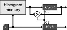
Another statistic that requires the histogram is the mode. The mode is defined as the index of the highest peak within the histogram. This requires a single scan through the histogram, for example as in Figure 7.10.
Figure 7.10 Finding the mode of a histogram.
There are two limitations to this approach for finding the mode. If the histogram is multimodal, only the global mode is found. The global mode is the one with the highest peak, which is not necessarily the most significant peak. Finding multiple peaks requires detecting the significant valleys and finding the mode between these valleys. Valley detection is described in Section 7.1.4 on threshold selection.
A second limitation is that histograms tend to be noisy. This is clearly seen in Figure 7.1. Consequently, the mode may not necessarily be representative of the true location of the peak. The accuracy of the peak location may be improved through filtering the histogram before finding the mode. A one-dimensional linear smoothing filter may be pipelined between reading the histogram values and finding the maximum. Suitable filters are described in detail in the next chapter. Note that care must be taken when designing the filter response to avoid bias being introduced if the peak is skewed.
7.1.2 Histogram Equalisation
Histogram equalisation is a contrast enhancement or contrast normalisation technique. It uses the histogram to construct a monotonic mapping that results in a flattened output histogram. From an information theoretic perspective, histogram equalisation attempts to maximise the entropy of an image by making each pixel value in the output equally probable.
From a contrast enhancement perspective, the assumption behind histogram equalisation is that the peaks of the input histogram contain the information of interest and the contrast between the peaks is of lesser importance. To make the output histogram flat, it is necessary to reduce the average height of the peaks by spreading the pixel values out. This increases the contrast of these regions. The valleys between the peaks are compressed to raise the average value, effectively reducing the contrast of these features.
These factors are clearly seen in Figure 7.11, where the regions with counts greater than the average are enhanced at the expense of those below the average. In this image, the effect has been to enhance the contrast within the background material; this is probably not the intended consequence for this image, where it would have been more useful to enhance the contrast between the regions. However, in many applications, histogram equalisation gives a useful contrast enhancement.
Figure 7.11 Histogram equalisation. Top: input image with its histogram; bottom: the image and histogram after histogram equalisation. The grey line on the histograms shows the average ‘flat’ level.
Note that the main peak of the output histogram is exactly the same height as that of the input. This is a consequence of using a point operation to perform the mapping, which requires all pixels with one value in the input to map to the same value in the output. The average is obtained by spacing consecutive input values to more separated values in the output. The opposite occurs for bins with counts below the average. Several consecutive input pixel values may map to the same output pixel.
A flatter histogram may be obtained by using local information to distribute the pixels with an input value with a large count over a range of output pixel values (Hummel, 1975; 1977) although such operations are technically filters rather than point operations.
The mapping for performing histogram equalisation is the normalised cumulative histogram. Intuitively, if the input bin count is greater than the average, the slope of the mapping will be greater than one, and conversely if less than the average. Normalisation requires scaling the histogram by the number of pixels, so that the output maps to the maximum pixel value (V).
The associated division operation is the most expensive part of histogram equalisation, although it can readily be pipelined. An alternative to division is to calculate the inverse off-line (since the number of pixels in an image is constant) and use a multiplication. Another alternative is to arrange the region of the image that the histogram is taken of to result in a scale factor that is a power of two. The region used is best taken from the centre of the image, with the assumption that the values not accumulated will follow the same statistics.
The division may be performed using repeated subtraction. This takes advantage of the fact that the cumulative histogram is monotonic to extend the calculations performed at lower pixel values to higher values. Therefore, the repeated subtractions calculate the mapping at the same time as the total is accumulating.
The architecture for this is shown in Figure 7.12. The counters map and i are initialised to zero, and the sum is initialised to −scale (or −scale/2 for rounding) where:
(7.18) ![]()
Figure 7.12 Using repeated subtraction to avoid division for histogram equalisation.
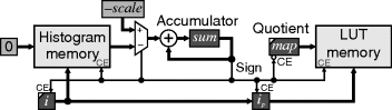
If the accumulated sum, which represents the current remainder, is negative then the count from the next histogram bin is accumulated. However, if the accumulated sum is positive, the scale factor is subtracted from the sum and the quotient incremented. When the index i is incremented, the previous value is also saved as ip. As a histogram bin is accumulated, the current quotient, map, is saved at the index ip. For 8-bit images, map will be incremented at most 255 times, and 257 clock cycles are required to read the input histogram and write the mapping into the lookup table.
There are several control issues associated with histogram equalisation, or indeed any other histogram processing. Firstly, the circuitry for building the histogram (for example from Figure 7.3 or Figure 7.4) must be combined with that for building the mapping used to perform the histogram equalisation (Figure 7.12). This will require appropriate multiplexers in the address and data lines. It is also necessary to reset the histogram accumulators to zero before the next frame. This may be accomplished in parallel with building the map, by using the histogram memory write port, as shown in Figure 7.12.
Secondly, there is a similar resource sharing issue with the mapping associated with performing the histogram equalisation. The lookup table must be shared between the circuit for building the mapping (Figure 7.12) and applying the mapping to the image. Each of these processes only requires a single port, so use of a dual-port memory would simplify the sharing. Otherwise, the map address lines would require an appropriate multiplexer, with additional control required to provide the memory read or write signal.
Thirdly, the registers for building the map (in Figure 7.12) may be initialised to appropriate values while the histogram is being built.
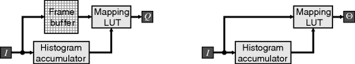
Finally, since construction of the histogram equalisation map requires data from the complete image, it is necessary to buffer the image before the mapping is applied, as shown in the left panel of Figure 7.13. In many instances, the image changes relatively slowly. An approximation in these circumstances is to apply the mapping acquired from the previous frame while building the histogram for the current frame (McCollum et al., 1988), as illustrated in the right panel of Figure 7.13. The consequence is that the histogram equalisation might not be quite correct, but there is a significant savings in both resources (the frame buffer is not required) and latency.
Figure 7.13 Using the histogram for histogram equalisation. Left: buffering the frame during histogram accumulation; right: directly applying table from the last image to the current image.
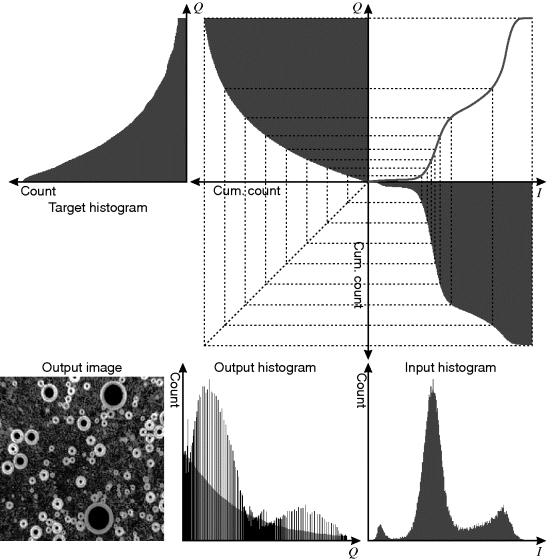
The procedure for histogram equalisation may readily be adapted to perform other histogram transformations, for example hyperbolisation (Frei, 1977). It is even possible to derive a target histogram from one image and apply a mapping to another image such that the histogram of the output image approximates that of the target. The basic procedure for this is illustrated graphically in Figure 7.14. To derive a monotonic mapping, it is necessary for all of the pixels less than or equal to a pixel value in the input image to map to values that are less than or equal to the corresponding output value. This may be achieved by mapping the cumulative histogram of the input to the cumulative histogram of the target. As with histogram equalisation, the output histogram approximates the target on average, as shown in the bottom of Figure 7.14.
Figure 7.14 Determining the mapping to produce an arbitrary output histogram shape by matching cumulative histograms. Top: target histogram and cumulative histogram; right: input histogram and cumulative histogram; top right: building the mapping; bottom: output image and output histogram (with target histogram in the background).
The circuit of Figure 7.12 may be adapted to calculate this mapping. Rather than subtract off the constant scale, the value to be subtracted may be obtained from the target histogram, ![]() (assuming that both images have the same area).
(assuming that both images have the same area).
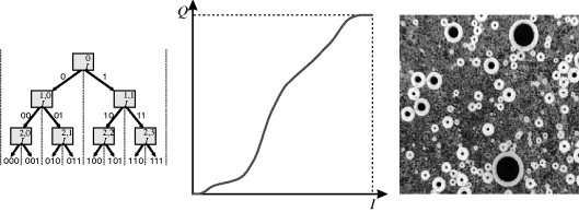
Related to histogram equalisation is the successive mean quantisation transform (Nilsson et al., 2005b). This works by using a series of means to derive successive threshold levels that define successive bits of the output pixel value. Initially, the whole range of pixel values is defined as a single partition. The mean value of the pixels within a partition is used to split the partition into two at the next level, with the corresponding output bit defined by the partition to which a pixel is assigned. This partitioning process is shown in Figure 7.15. Sum tables may be used to calculate successive means efficiently using Equation 7.13.
Figure 7.15 Determining the output code or pixel value using the successive mean quantisation transform. Centre: the resultant mapping; right: applying the mapping to the input image. (Adapted with permission from M. Nilsson et al., “The successive mean quantization transform,” IEEE International Conference on Acoustics, Speech and Signal Processing, 4, 429–432, 2005. © 2005 IEEE.)
It has been demonstrated that, in many applications, the successive mean quantisation transform provides a subjectively better enhancement than histogram equalisation, because it preserves the gross structure of the histogram and does not over-enhance the image (Nilsson et al., 2005a; 2005c). In the context of the successive mean quantisation transform, histogram equalisation corresponds to successively partitioning using the median rather than the mean.
7.1.3 Automatic Exposure
Related to contrast enhancement is automatic exposure. This involves using data obtained from the captured image to modify the image capture process to optimise the resultant images. In sensors with electronic shuttering, this may require adjusting the control signals that determine the exposure time. It may also involve automatically adjusting the aperture or even controlling the intensity of the light source.
The histogram of the captured image is able to provide useful data for gauging the quality of the exposure. If the maximum pixel value within the image is significantly less than V, then the image is not making the best use of the available dynamic range. This may be improved by increasing the exposure. On the other hand, if the image contains a large number of pixels with pixel value V, then there may be important detail lost through saturation. This may be corrected by reducing the exposure.
Although the maximum pixel value may be determined without needing a histogram, there are two major limitations to using the maximum pixel value to assess exposure. Firstly, the maximum value is likely to be a result of noise and may not reflect the true peak of intensities within the image. Secondly, the maximum pixel value may actually reach V without being saturated. In many images, the maximum value may result from specular reflections or other highlights that are not significant from an image processing point of view.
An alternative approach is to use the histogram to find the pixel value of the 99th percentile (Bailey et al., 2004) (or even higher depending on the image content). If the histogram is flat, the 99th percentile should have a value of about 252 for an 8-bit image. However, most histograms are non-uniform, and in many applications there may be variability from one frame to the next that must be tolerated.
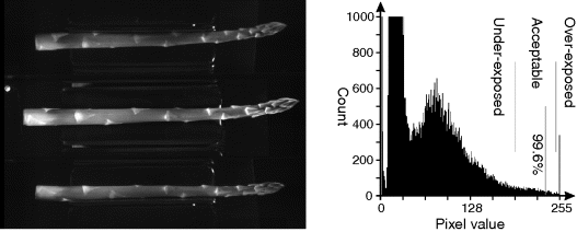
One approach is to have a target acceptable range for the given level. Consider the image in Figure 7.16. The histogram clearly shows that some pixels are saturated (from the peak at 255). These are the specular reflections and highlights in the figure on the left, and no information of importance is lost if these are saturated. However, the 99.6th percentile (allowing for the equivalent of two rows worth of pixels to be saturated) is within the allowed band of 192–250, indicating that the exposure for this image is acceptable. In this application, the large dead-band allowed for the considerable variability in the produce from one image to the next, while ensuring that an adequate exposure was maintained.
Figure 7.16 Using the histogram for exposure. Left: example image; right: histogram with its 99.6th percentile shown, along with the acceptable bounds.
When determining if the exposure is acceptable, it is faster to accumulate the histogram counts starting from the maximum pixel value and counting down, rather than counting up from zero.
Note that changing the camera exposure will not affect the current image. It may also be best to adjust the exposure incrementally over several images rather than in a single step, especially if the object being imaged changes from one image to the next.
7.1.4 Threshold Selection
The purpose of thresholding is to segment the image into two (or more) classes based on pixel value. While it is possible to consider connectivity and other issues (Sezgin and Sankur, 2004), there is a wide range of threshold selection techniques that calculate a threshold level from the histogram rather than the image (Sezgin and Sankur, 2004). Consider an obvious case, where the pixel values of each class are well separated; the resulting pixel value histogram is multimodal. This implies that the distributions of each of the classes, and hence the best places to threshold the image, may be determined by analysing the histogram. Since selecting an appropriate threshold is a common task in many image analysis applications, many of the key methods for dynamically determining the threshold from a histogram will be reviewed.
The most common case is separating objects from a background, where there are two classes: object and background. If the proportion of object pixels is known then the corresponding threshold level may be determined from the inverse cumulative histogram (Doyle, 1962). This may be found from the cumulative histogram in two ways.
The first is to scan through cumulative histogram until the desired proportion is reached. In fact, it is not necessary to actually build the cumulative histogram; the histogram counts may be accumulated until the desired total is reached.
The second approach, if the cumulative histogram is available, is to solve Equation 7.19 using a binary search, as described earlier for finding the median.
In many cases, however, the number of object pixels in not known in advance, but is determined as a result of thresholding. An alternative that is more tolerant of variation in the number of object pixels is to set the threshold a given number of standard deviations from the mean:
(7.20) ![]()
where ![]() is chosen empirically based on knowledge of the image being thresholded.
is chosen empirically based on knowledge of the image being thresholded.
When separating objects from the background, the histogram is often bimodal, with the peaks representing the distributions of object and background pixel values. If the peaks are clearly separated and do not overlap, choosing an appropriate threshold between the peaks is relatively trivial. In most cases, however, the peaks are often broad, with significant overlap between the distributions, as in the image in Figure 7.17. When the histogram has distinct peaks, an appropriate threshold is somewhere in the valley between the peaks. Finding the ‘best’ threshold is complicated by the fact that the histogram is seldom smooth. Both the peaks and the valley between them are noisy, so simply choosing the deepest valley can result in considerable variation from one image to the next.
Figure 7.17 An image of objects against a background and its corresponding histogram.
One approach to this problem is to smooth the histogram to make the valley between the peaks clearer. This was first proposed by Prewitt and Mendelsohn (1966). The histogram is repeatedly filtered with a narrow filter until there are only two maxima; the threshold is then in the valley between the peaks. That is, it will be the only pixel value in the histogram that satisfies:
A variation on this theme is to record the location of the peaks and valleys and track these through a range of filter widths. This results in a range of thresholds, depending on the scale of filtering (Carlotto, 1987). Such a multiscale approach suits multilevel thresholding, or the threshold at the lowest scale (most smoothed) may be tracked up the scales to refine it. A disadvantage of such approaches is the repeated filtering required to obtain the necessary smoothness, or range of scales in the latter case.
An alternative approach is to fit a curve to the histogram. A common assumption is that the shape of each of the modes is a Gaussian distribution, modelling the histogram as a sum of Gaussians:
(7.22) ![]()
In the case where the histogram is bimodal, the threshold that gives the minimum misclassification error is (Kittler and Illingworth, 1986):
where
(7.24) 
and
(7.25) ![]()
This is based on separating the histogram into two parts by the threshold and modelling each part with a Gaussian distribution. The minimum error will correspond to the crossover point between the two distributions. Jiulun and Winxin (1997) showed that the derivation given by Kittler is equivalent to minimising the relative entropy between the actual distributions and the ideal Gaussian distributions and determining the threshold that gives the minimum classification error.
Equation 7.23 may be evaluated with a single pass through the cumulative histogram, although several clock cycles may be needed for each t to evaluate the logarithms. Note the square roots for calculating the standard deviation may be avoided by using:
(7.26) ![]()
An alternative to fitting to the histogram is to make the distributions on each side of the threshold as compact as possible. This leads to the popular approach by Otsu of minimising the intra-class variance (Otsu, 1979):
which is equivalent to maximising the separation between the means, or the interclass variance:
where
(7.29) ![]()
The advantage of Equation 7.28 over Equation 7.27 is that is only requires calculating the means rather than the variances. Since the criterion function that is maximised in Equation 7.28 can have multiple local maxima (Lee and Park, 1990), iterative methods for finding the maximum may converge to the wrong value. Therefore, it is necessary to search by scanning through the histogram. Equation 7.28 may be calculated incrementally if the global mean is known. Firstly, a pair of registers is initialised to zero:
(7.30) ![]()
Then the following iterations are used:
Note that in Equation 7.31 p1 is not a probability, rather it is the cumulative histogram. The division by NP is unnecessary, since it is constant and will not affect the location of the maximum.
Alternatively, the criterion function may be evaluated directly from the cumulative histogram and summed first moment:
Again, the factor of ![]() in the denominator of the first two terms may be left out and Equation 7.32 rearranged to reduce the number of division operations:
in the denominator of the first two terms may be left out and Equation 7.32 rearranged to reduce the number of division operations:
(7.33) ![]()
Otsu's method works best with a bimodal distribution, with a clear distinct valley between the modes (Lee and Park, 1990). Performance can deteriorate when there is a significant imbalance between the number of object and background pixels, or when the object and background are not well separated, or when there is significant noise (Lee and Park, 1990).
In principle, Otsu's method may be extended to multilevel thresholding (Otsu, 1979), although each threshold added will increase the dimensionality of the search space, making the search for the maximum computationally impractical for more than two or three threshold levels. Peaks within the multidimensional criterion function will correspond to zero partial derivatives, and iterative search techniques may be employed to speed up the search for the zero partial derivatives (Lin, 2005).
An alternative approach that gives similar results to Otsu's method for many images is to iteratively refine the threshold to midway between the means of the object and background classes (Ridler and Calvard, 1978; Trussell, 1979):
with the initial threshold given from the global mean:
The iteration of Equation 7.34 is repeated until it converges (![]() ), although this generally occurs within four iterations (Trussell, 1979). Note that the resultant threshold level is dependent on the initial value. The initialisation of Equation 7.35 works well if there are approximately equal numbers of object and background pixels, or the object and background are well separated. An alternative initialisation if the distribution is very unbalanced is the midrange of the distribution:
), although this generally occurs within four iterations (Trussell, 1979). Note that the resultant threshold level is dependent on the initial value. The initialisation of Equation 7.35 works well if there are approximately equal numbers of object and background pixels, or the object and background are well separated. An alternative initialisation if the distribution is very unbalanced is the midrange of the distribution:
(7.36) ![]()
The attractiveness of this iterative method is its simplicity and speed, and with good contrast images it gives good results.
Another approach to thresholding is to use the total entropy of two regions of the histogram as the criterion function (Kapura et al., 1985). The threshold is then chosen to maximise the information between the object and background distributions:
As with the other methods, calculating the optimum threshold using this criterion function may be performed with a single pass through the histogram. However, as with the minimum error method, a hardware implementation is complicated by the need to calculate logarithms. Maximising the entropy has a tendency to push the threshold towards the middle of the distribution, so this method works best when there is a clear distinction between the two distributions. It may also be extended to multilevel thresholding (Kapura et al., 1985) in a similar manner to Otsu's method, with the same limitation of the exponential growth of the search space with the number of threshold levels used.
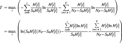
When the object and background distributions significantly overlap, there may not be two distinct modes to the distribution. Rosenfeld and de la Torre (1983) proposed using the difference between the distribution and its convex hull to identify irregularities on the flanks of a unimodal distribution. The method also works equally well with bimodal distributions, where it will tend to bias the threshold toward the higher peak, as shown in Figure 7.18. Since, in general, the convex hull is sloped, the largest difference will correspond to the pixel value in the valley that has a tangent parallel with the hull. It is this slope that biases the threshold location and enables a bump on the side of a unimodal histogram to be detected.
Figure 7.18 Convex hull of histogram. Left: the convex hull superimposed on the histogram, the line parallel to the top of the hull shows how the threshold is biased towards the higher peak; right: the difference between the hull and the histogram.
The convex hull of the histogram is the smallest extension of the shape that has no concavities. A physical analogy is to stretch a rubber band over the histogram and fill in the histogram below the rubber band, as shown in Figure 7.18. The convex hull may be represented by the set of convex vertices, which corresponds to the set of counts in the histogram that are unaffected by this infilling process.
Firstly, observe that the slope of the convex hull decreases monotonically with increasing pixel value. Therefore, consider a sequence of three points with increasing pixel value: ![]() ,
, ![]() and
and ![]() . The middle point is concave if the slope between the first two points is less than the slope between the second two points. That is:
. The middle point is concave if the slope between the first two points is less than the slope between the second two points. That is:
(7.38) ![]()
The division may be avoided by cross-multiplying:
If the middle point is concave, it may be eliminated.
Using this, the convex vertices may be found as follows. Firstly, the histogram is scanned to find the first non-zero count and the corresponding pixel value, ![]() , is stored in a register. For each successive pixel value, the pixel difference,
, is stored in a register. For each successive pixel value, the pixel difference, ![]() and histogram difference,
and histogram difference, ![]() , are determined. A table is used to maintain these offsets between the convex vertices. If the table is empty, the pair
, are determined. A table is used to maintain these offsets between the convex vertices. If the table is empty, the pair ![]() is recorded in the table. If the table is not empty, Equation 7.39 is evaluated between the last entry in the table and the new entry:
is recorded in the table. If the table is not empty, Equation 7.39 is evaluated between the last entry in the table and the new entry:
If Equation 7.40 is true, then the previous vertex is now concave so must be eliminated. The last entry in the table is therefore removed and combined with the current entry:
Equation 7.40 is repeatedly re-evaluated with the new last entry in the table and entries removed with Equation 7.41 until all concave vertices to the left of the current point are removed. Then the current point is added to the table. Note that when a count of zero is reached (![]() ), the above is not performed in case it is the end of the histogram. However, if a subsequent non-zero count is encountered,
), the above is not performed in case it is the end of the histogram. However, if a subsequent non-zero count is encountered, ![]() is set to reflect the intervening zero counts.
is set to reflect the intervening zero counts.
Once the end of the histogram has been reached, the table will contain the offsets between the convex vertices. This process will take at most 2V steps, because for each new pixel value one entry is added to the table, and through the elimination steps each entry can only be removed at most once from the table.
The final stage is to link between the convex vertices to obtain the convex hull. This is complicated slightly by the fact that the pixel values are discrete and the slopes are not necessarily represented by integers. This process starts with the pixel value with the first non-zero count, ![]() , and initialising a remainder to zero:
, and initialising a remainder to zero:
(7.42) ![]()
Then each table entry is used to calculate the next ![]() hull values:
hull values:
(7.43) 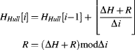
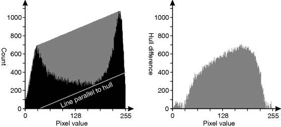
where ![]() is the largest integer value less than its argument, and mod returns the remainder between zero and
is the largest integer value less than its argument, and mod returns the remainder between zero and ![]() . Rather than record the actual hull, it is only necessary to determine the pixel value corresponding to the maximum difference between the hull and the original histogram
. Rather than record the actual hull, it is only necessary to determine the pixel value corresponding to the maximum difference between the hull and the original histogram
that is, the position of the maximum value on the right in Figure 7.18.
A variation on valley finding is the global valley approach of Davies (2008). His criterion function is based on the geometric mean of differences between a histogram point and the peaks on either side:
where
(7.46) 
and
(7.47) ![]()
The geometric mean in Equation 7.45 is better than the arithmetic mean because it prevents pedestals at the ends of the distribution (Davies, 2008). Only two passes are required through the histogram to evaluate the criterion function: a reverse pass to incrementally calculate HR and a forward pass to incrementally calculate both HL and the criterion function. If searching for a single threshold, the square root operation of Equation 7.45 may be omitted.
This approach may be extended to multilevel thresholding by smoothing the criterion function until the specified number of local maxima remains (Davies, 2008).
The threshold levels calculated for the different methods are compared in Figure 7.19 for the image of Figure 7.17. The different assumptions made, and different criteria functions, result in threshold levels ranging from 127 for the maximum entropy method, through to 188 for the minimum error method. Note that for this image there is no global threshold that provides good separation between the objects and the background. Of all the methods considered here, the iterative mean of Equation 7.34 is computationally the simplest, especially if the cumulative histogram and the cumulative first moment are calculated.
Figure 7.19 Applying the threshold calculation method to the histogram of Figure 7.17. The methods are minimum error (Equation 7.23), convex hull (Equation 7.44), smoothed minimum (Equation 7.21), Davies (Equation 7.45), iterative mean (Equation 7.34), Otsu (Equation 7.28) and entropy (Equation 7.37). Right: results of the two extreme threshold levels are compared; top: the minimum error method; bottom: the maximum entropy method.
Histogram-based methods of calculating threshold levels generally rely on valley finding techniques. If the number of either object or background pixels is significantly smaller than the other, the valley between the peaks can be indistinct. Filters may be applied to the image to improve the histogram obtained. Obtaining the histogram-only pixels near edges will result in an approximately equal numbers of object and background pixels (Weszka et al., 1974). Noise smoothing may result in narrower peaks, making them more distinct and easier to detect and separate. Applying an edge enhancement filter prior to accumulating the histogram will reduce the number of pixel values in the valley between the peaks, making the result less sensitive to the actual threshold level used (Bailey, 1995).
Many of the threshold selection techniques described here would be easier to implement in software, using an embedded processor, than directly in hardware. The timing is not particularly critical because the threshold could be calculated during the vertical blanking period between frames.
Only global thresholding has been considered in this section. Adaptive thresholding chooses a different threshold at each location based on local statistics. Adaptive thresholding can be considered equivalent to filtering followed by global thresholding. Adaptive thresholding is considered in more detail in the next chapter on filtering.
7.1.5 Histogram Similarity
Histogram similarity is one method of object classification. The intensity histograms of a set of candidate model objects are maintained in a database. The histogram of the test object is obtained and compared with the histograms of the model objects, with the object classified based on which model has the most similar histogram. Unlike most other methods of object classification, the object does not need to be completely separated from the background, as long as it dominates the content of the image.
The histogram may require some normalisation prior to matching (usually limited to contrast stretching) to account for varying illumination intensity. Normalisation such as histogram equalisation, or shaping, is obviously not appropriate. Often the resolution of the histogram is reduced (the bin size is increased) by combining adjacent bins. This reduces the sensitivity to small changes in illumination and reduces problems resulting from gaps in the histogram that result from normalisation. It also helps to speed the search for a match.
Let all the model histograms be normalised to correspond to the same area image and let ![]() be the histogram of the jth model. The similarity between the test histogram,
be the histogram of the jth model. The similarity between the test histogram, ![]() , and the model can be found from their intersection (Swain and Ballard, 1991):
, and the model can be found from their intersection (Swain and Ballard, 1991):
This measure will be a maximum when the histograms are identical and will decrease as the histograms become more different. Therefore, the input image is classified as the object that has the largest match.
All spatial relationships between the pixel values are lost in the process of accumulating the histogram. Consequently, many quite different images can have the same histogram. Classification based on histogram similarity will, therefore, only be effective when the histograms of all of the models are distinctly different. However, the method has the advantage that the histogram has a considerably smaller volume of data than that of the whole image, significantly reducing comparison times. This can be helped further by reducing the number of bins within the histograms. Where speed is important, the test histogram may be compared with a number of model histograms in parallel.
7.2 Multidimensional Histograms
Just as pixel-value histograms are useful for gathering data from greyscale images, multidimensional histograms can be used to accumulate data from colour or other vector valued images. The simplest approach is simply to accumulate a one-dimensional histogram of each channel. While this is useful for some purposes, for example gathering the data required for colour balancing, it cannot capture the relationships between channels that give each pixel its colour. This requires a true multidimensional histogram.
A multidimensional histogram has one axis or dimension for each channel in the input image. For example, the histogram of an RGB image would require three dimensions. The histogram gives a count of the pixels within the image that have a particular vector value. For an RGB image, Equation 7.1 would be extended to give:
(7.49) ![]()
Data is accumulated in exactly the same way as for a greyscale histogram. The larger address space of a multidimensional histogram requires a significantly larger memory, which may not necessarily fit within the FPGA. Two histogram memory accesses are required for each pixel: one to read the previous count and the other to write the updated count. This may be accomplished either with dual-port memory, in the same manner as one-dimensional histograms (Figure 7.4), or by running the accumulator memory at twice the pixel clock frequency.
While it is usually possible to implement two-dimensional histograms at the full resolution of the input vector, for three and higher dimensions the size of the histogram memory can become prohibitively large. This problem may be overcome by reducing the number of bins by applying a coarse quantisation to each component. Indexing into the multidimensional array is performed in the same manner as in software:
(7.50) ![]()
where ![]() and
and ![]() are the number of bins used for the x and y components, respectively. Indexing may be simplified if the range of each component is a power of two, as the memory address may then be formed by concatenating the vector components. The quantisation to accomplish this may be readily implemented by truncating the least significant bits of each vector component.
are the number of bins used for the x and y components, respectively. Indexing may be simplified if the range of each component is a power of two, as the memory address may then be formed by concatenating the vector components. The quantisation to accomplish this may be readily implemented by truncating the least significant bits of each vector component.
One limitation with using multidimensional histograms is the time required to both initialise them and to extract the data. Throughput issues may be overcome by using pipelining, although bandwidth issues are harder to deal with. It may require multiple parallel banks to initialise and process the histograms in a realistic time. Bank switching allows one bank to be initialised while another is accumulating and a third is being processed. Once the histogram data has been collected, the histograms can be used and processed as images in their own right if necessary.
7.2.1 Triangular Arrays
Often when processing colour images, intensity independence is often desired. With an appropriate colour space conversion, the intensity may be removed, with a reduction to two dimensions for the chrominance. If chromaticity is used (either ![]() or
or ![]() ) the resulting histogram accumulator is triangular. This may result in inefficient use of memory, as almost half is not being used. Unless the memory may be shared with another part of the application, an alternative is to pack the memory.
) the resulting histogram accumulator is triangular. This may result in inefficient use of memory, as almost half is not being used. Unless the memory may be shared with another part of the application, an alternative is to pack the memory.
With a triangular accumulator, ![]() . The number of entries in the triangular array is then
. The number of entries in the triangular array is then ![]() rather than
rather than ![]() for the full array. When n is a power of two, as suggested earlier for efficiency, say
for the full array. When n is a power of two, as suggested earlier for efficiency, say ![]() , the number of entries becomes:
, the number of entries becomes:
If using a single memory block, this does not result in any savings, because of the second term in Equation 7.51. Memory savings can only be achieved with multiple small memory blocks.
Instead, if the number of bins is reduced to ![]() , the number of entries is now:
, the number of entries is now:
(7.52) ![]()
Since the second term is now subtracted rather than added, the array will fit into a block of size ![]() .
.
The quantisation of the input range into ![]() bins is now more complex and requires scaling the input before truncating the least significant bits. Fortunately, this scaling may be implemented by a single subtraction:
bins is now more complex and requires scaling the input before truncating the least significant bits. Fortunately, this scaling may be implemented by a single subtraction:
(7.53) ![]()
Two approaches may be used to pack the data into the smaller array. The first successively shifts each row back in memory to remove the unused entries:
(7.54) 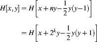
The multiplication may be avoided by using a small lookup table on the y address, as shown on the left in Figure 7.20.
Figure 7.20 Packed addressing schemes for a triangular array with ![]() . Left: packing the rows sequentially. The numbered memory locations represent the addresses stored in the Addr LUT. Right: folding the upper addresses into the unused space.
. Left: packing the rows sequentially. The numbered memory locations represent the addresses stored in the Addr LUT. Right: folding the upper addresses into the unused space.
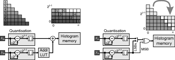
The second approach is to maintain the spacing but fold the upper addresses into the unused space at the end of each row:
(7.55) 
Note that ![]() and
and ![]() are just one's complements of x and y respectively, enabling them to be implemented with exclusive OR gates as shown in Figure 7.20.
are just one's complements of x and y respectively, enabling them to be implemented with exclusive OR gates as shown in Figure 7.20.
7.2.2 Multidimensional Statistics
The scalar mean and variance extend to vector valued quantities as the mean vector and covariance matrix. The mean vector is simply found by taking the mean of the components, for example the mean of a three-dimensional data set is:
(7.56) 
Similar to the variance of Equation 7.4, the covariance between two variables is:
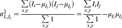
with the covariance matrix formed from the covariances between every pair of components:
(7.58) 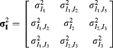
The diagonal elements of ![]() correspond to the variances of the individual components. The off-diagonal elements measure how the corresponding components vary with respect to each other, which reflects the correlation between that pair of components. It is clear from Equation 7.57 that the covariance matrix is symmetric. In matrix form:
correspond to the variances of the individual components. The off-diagonal elements measure how the corresponding components vary with respect to each other, which reflects the correlation between that pair of components. It is clear from Equation 7.57 that the covariance matrix is symmetric. In matrix form:
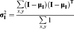
where the superscript ![]() denotes the vector transpose. (For complex data, the complex conjugate of the transpose is used.)
denotes the vector transpose. (For complex data, the complex conjugate of the transpose is used.)
For a colour image, each sample has three components or dimensions. Calculating the mean therefore requires three accumulators, one for each dimension. If the denominator is not fixed (for example extracting statistics from a region of the image), an additional accumulator is required for the denominator. From the symmetry in the covariance matrix, only six accumulators are required for the numerator of Equation 7.59.
When calculating global statistics for the image, the data for the mean and covariance may be performed directly on the input as it is streamed in. Alternatively, a multidimensional histogram may be used as an intermediary, in a similar manner to that described in Section 7.1.1. While using a histogram as an intermediate step is efficient for one-dimensional histograms, in two and higher dimensions their utility for this purpose becomes marginal. Unless the resolution in each dimension is reduced, the histogram can have more entries than the original image. While this may be overcome by reducing the resolution, this will also reduce the accuracy of the statistics derived from the histograms. Therefore, gathering data from a multidimensional histogram is usually only practical if many separate calculations must be performed for different regions within the multidimensional data space (for example to obtain the mean and covariance for each of a set of colour classes).
The covariance matrix may be used in a number of ways. If the covariance matrix is of a set of points from the same distribution, such as from the same colour class, then the covariance matrix provides information on the spread of distribution within the multidimensional space. If the distribution is Gaussian, then the shape will be ellipsoidal, with the orientation and extent of the ellipsoid defined by the covariance matrix. In one dimension, the probability that a point, x, belongs to the distribution may be determined from the distance of the point from the centre of the distribution, d, in terms of the number of standard deviations:
With a multidimensional distribution, in general the spread of the distribution is different in different directions. The Mahalanobis distance (Mahalanobis, 1936) generalises Equation 7.60 to measure the distance of a vector, x, from a distribution, X, using the covariance:
(7.61) ![]()
If the distribution is spherical, with a standard deviation of one, then the covariance matrix will be the identity matrix, and this will reduce to the standard Euclidean distance:
(7.62) ![]()
Another common use for the covariance matrix is for dimensionality reduction. Principal components analysis (PCA) defines a new set of axes where each axis is independent of the others (the covariances are all zero). This effectively rotates the multidimensional space in such a way to best align the axes with the axes of the distribution. In the rotated space, the axes are ordered in terms of decreasing variance. This means that the first principle component is in the direction that accounts for the most variation within the data, and corresponds to the long axis of the ellipsoid if the data is from a multidimensional Gaussian distribution. The dimensionality of the data set may be reduced by discarding the lower order components. It can be shown that for a given number of dimensions or axes retained, this will minimise the error of the approximation in a least squares sense.
The principal component axes are found by determining the eigenvectors of the covariance matrix. It can be shown that the eigenvectors will be orthogonal because the covariance matrix is symmetric. Therefore, the matrix E formed from the unit eigenvectors of the covariance matrix will represent a pure rotation of the multidimensional space about the centre (or mean vector). The corresponding eigenvalues represent the variance in the direction of each eigenvector. This is related by:
(7.63) ![]()
where the ![]() is the diagonal covariance matrix of the transformed data. The transformation is performed by projecting each pixel onto the new axes:
is the diagonal covariance matrix of the transformed data. The transformation is performed by projecting each pixel onto the new axes:
The complexity of the control logic for determining the eigenvectors from the covariance matrix implies that this step is probably best performed in software rather than hardware. Of course, the ALU for the processor may be enhanced with dedicated instructions to accelerate the matrix operations. Once the transformation matrix, E, has been determined, the projection of Equation 7.64 may be readily implemented in hardware.
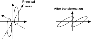
The principal components are only independent axes with respect to the underlying data only if the whole data set is Gaussian distributed. This may be the case if it is performed on a cluster of data points within the data set (for example a particular colour class) but is generally not the case for whole images, which consist of multiple objects or classes. In this case, PCA will merely decorrelate the axes. These axes may not necessarily have any useful meaning; in particular, they may not necessarily be useful features for performing classification. The two-dimensional (contrived) example of Figure 7.21 is such a counter-example that illustrates a case where the original axes were better for separating the two classes than the principal axes.
Figure 7.21 Principal components counter-example. Left: the data on the original axes, with the principal component axes overlaid. The ellipses represent different data classes. Right: after PCA transformation; the original axes were better for class separation than the PCA axes.
From an image processing perspective, principal components analysis has two main uses. When applied across the components of an image, it determines the linear combinations of components that account for most of the variation within the image. This may be used, for example, to reduce the number of channels of a multispectral image. It can also be used for image compression to concentrate or compact the energy in the signal. Fewer bits are required for the components that have lower variance. In this regard, the principal components of an RGB image are often similar to the YUV or YIQ components (unless the image is dominated by a strongly coloured region).
The second application of PCA is in object recognition. In this case, rather than consider the components as the axes, the pixel locations are the axes; each image may then be considered a point in this very high dimensional space. When considering a set of images of related objects, each image will result in a separate point, with the resulting distribution representing the variability from one image to another. The dimensionality of this high dimensional space may be significantly reduced by principal components analysis. Each axis in the new space corresponds to an eigen-image – the high dimensional eigenvector of the corresponding covariance matrix. The variation between the set of images may be reduced to a small number of components, representing the projections onto, hence the weights of, each eigen-image. These weights may then be used for classifying the objects. One classic example of this approach is face recognition (Turk and Pentland, 1991), where the eigen-images are often referred to as eigen-faces.
Other statistical measures, such as the median and range, are based on an ordering of the data. Since vectors have no natural ordering (Barnett, 1976), the standard definitions no longer apply. The simple approach of taking the median or range of each component gives an approximation but is not the true result. For the median, the resulting point may not be one of the input data points because in general the median of one component will select a different pixel to the median of another component (Astola et al., 1990). When used for median filtering within an image, this can result in coloured fringes around edges.
The problem with operating independently on the components is that it does not take into account the relationship between components. Each vector value should be treated as a single unit and operated on as such. One approach is to convert the vector to a scalar, which can then be used to define an ordering. Such conversions enable a reduced ordering (Barnett, 1976), with the results determined by the particular conversion used. A simple conversion is to use the vector magnitude. For colour images, the luminance, or in fact any weighted combination of the components, could be used as the scalar value for ordering (Comer and Delp, 1999). A limitation of these approaches is that many quite different vectors would be considered equal, with no ordering between them. One way of overcoming this for integer components is to interleave the bits of each of the components (Chanussot et al., 1999). This keeps each distinct vector unique, although the ordering is still dependent on interleaving order.
It is possible to define both a true median (Astola et al., 1988; 1990) and range (Barnett, 1976) for vector data. The median of a set of vectors, X, is the vector within the set, x, that minimises the distances to all of the other points in the set. That is:
The distances may be measured either using Euclidean (L2 norm) or city block (L1 norm) distances (Astola et al., 1990). The city block distance is easier to calculate in hardware, although the median vector will then depend on the particular coordinates used. Calculating the median requires measuring the distance between every pair of points within the set. This makes the computational complexity of order ![]() where N is the number of points in the set. For an image, this is impractical. However, for smaller N, such as filtering, this is more feasible.
where N is the number of points in the set. For an image, this is impractical. However, for smaller N, such as filtering, this is more feasible.
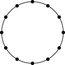
One limitation of the median defined in this way is that it is not unique. Consider a set of points distributed symmetrically (for example in two dimensions, evenly around the circumference of a circle as shown in Figure 7.22). Each one of the points is the median as defined by Equation 7.65. This non-uniqueness results from requiring the median to be one of the input samples. Davies (2000) argues that this constraint is unnecessary and results in selecting a point that is not representative of the data as a whole. If this constraint is relaxed, the resulting minimum, also called the geometric median, is then:
Figure 7.22 Vector median is not unique.
(7.66) ![]()
where n is the number of components in each vector. It can be shown that the geometric median is unique (Ostresh, 1978) and may be found iteratively by Weiszfeld's algorithm (Ostresh, 1978; Chandrasekaran and Tamir, 1989):
Each iteration of Equation 7.67 requires summing over the complete set of vectors. Since successive iterations must be performed sequentially, the only scope for parallelism is to partition the set of input vectors over several processors. Calculating the inverse Euclidean distance is also relatively expensive, but is amenable to pipelining using a CORDIC processor. The resulting weight may be shared by the numerator and denominator. The iteration of Equation 7.67 converges approximately linearly, although it can get stuck if one of the intermediate points is a one of the input vectors (Chandrasekaran and Tamir, 1989).
For multidimensional data, the range can be defined as the distance between the two points that are furthermost apart (Barnett, 1976):
(7.68) ![]()
Again the distance between every pair of points must be calculated, giving complexity of order ![]() . A simpler approximation is to combine the ranges of each component. This assumes that the distribution is rectangular and aligned with the axes, so will tend to over-estimate the true range.
. A simpler approximation is to combine the ranges of each component. This assumes that the distribution is rectangular and aligned with the axes, so will tend to over-estimate the true range.
7.2.3 Colour Segmentation
Multidimensional histograms provide a convenient visualisation for segmentation, particularly when looking at colour images. Segmentation is equivalent to finding clusters within the data set, or equivalently finding peaks within the multidimensional histogram.
When considering colour segmentation or colour thresholding, using three-dimensional histograms is both hard to visualise and expensive in terms of resources. In this case, pairs of components are usually considered; this projects the three-dimensional histogram onto a two-dimensional plane. As described before, RGB is generally not the best colour space for segmentation. If colour is of primary interest, then the colour can be converted to YCbCr or HSV and the intensity channel ignored. The corresponding two-dimensional histograms are then taken of either ![]() or
or ![]() respectively. Alternatively, the components can be normalised and the
respectively. Alternatively, the components can be normalised and the ![]() or
or ![]() histogram taken.
histogram taken.
Several of these are compared in Figure 7.23. Note the predominantly diagonal structure in the ![]() histogram in the left panel. This is even more exacerbated if the lighting varies across the scene. The grid structure is caused from the stretching of each component during colour correction.
histogram in the left panel. This is even more exacerbated if the lighting varies across the scene. The grid structure is caused from the stretching of each component during colour correction.
Figure 7.23 Example two-dimensional histograms of the colour corrected image from Figure 6.44. Left: ![]() histogram; centre:
histogram; centre: ![]() histogram; right:
histogram; right: ![]() histogram. (For key features of each histogram, refer to the text.)
histogram. (For key features of each histogram, refer to the text.)
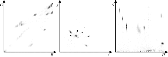
Normalising the coordinates by dividing the sum (as in Equation 6.78) gives the ![]() histogram. This is a triangular histogram with nothing above the line
histogram. This is a triangular histogram with nothing above the line ![]() . The intensity dependence has been removed, resulting in tighter groups. The dense group in the centre corresponds to the white background. The isolated ‘random’ points result from the black region where a small change in one of the components due to noise drastically changes the proportions of the components. Black regions must be distinguished based on luminance rather than colour. The faint lines connecting each cluster with the background result from mixing around the edges of each coloured patch; the edge pixels consist partly of the coloured object and partly of the background. Although present in all of the histograms, these edges are more visible in the
. The intensity dependence has been removed, resulting in tighter groups. The dense group in the centre corresponds to the white background. The isolated ‘random’ points result from the black region where a small change in one of the components due to noise drastically changes the proportions of the components. Black regions must be distinguished based on luminance rather than colour. The faint lines connecting each cluster with the background result from mixing around the edges of each coloured patch; the edge pixels consist partly of the coloured object and partly of the background. Although present in all of the histograms, these edges are more visible in the ![]() or
or ![]() histograms.
histograms.
The third example is the ![]() histogram on the right. This, too, removes the intensity dependence. The best separation is achieved after proper colour balancing, which has quite a strong effect on both the hue and saturation. The pattern of points at low saturation results from noise affecting both the hue and saturation of grey and white pixels. Similarly, the scattered points at higher saturation result from noise affecting the black pixels.
histogram on the right. This, too, removes the intensity dependence. The best separation is achieved after proper colour balancing, which has quite a strong effect on both the hue and saturation. The pattern of points at low saturation results from noise affecting both the hue and saturation of grey and white pixels. Similarly, the scattered points at higher saturation result from noise affecting the black pixels.
The colour histogram can then be used as the basis for segmentation. This process is illustrated in Figure 7.24 with the ![]() histogram (using Equation 6.61) of the colour corrected image of Figure 6.44. Since each of the coloured patches results in a distinct cluster, simply thresholding the two-dimensional histogram is effective in this case. Each connected component in the histogram is assigned a unique label (Section 11.4), represented here by a colour. This labelled two-dimensional histogram can then be used as a lookup table on the original U and V components to give the labelled, segmented image.
histogram (using Equation 6.61) of the colour corrected image of Figure 6.44. Since each of the coloured patches results in a distinct cluster, simply thresholding the two-dimensional histogram is effective in this case. Each connected component in the histogram is assigned a unique label (Section 11.4), represented here by a colour. This labelled two-dimensional histogram can then be used as a lookup table on the original U and V components to give the labelled, segmented image.
Figure 7.24 Using a two-dimensional histogram for colour segmentation. Left: ![]() histogram using Equation 6.61; centre: after thresholding and labelling, used as a two-dimensional lookup table; right: segmented image. (See colour version of this figure in colour plate section)
histogram using Equation 6.61; centre: after thresholding and labelling, used as a two-dimensional lookup table; right: segmented image. (See colour version of this figure in colour plate section)
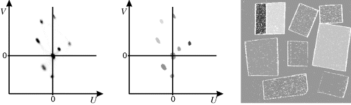
In the example here, the white pixels represent unclassified colour values. The corresponding points within the histogram were below the threshold. The number of unclassified pixels within a patch may be significantly reduced by expanding the labelled regions within the two-dimensional lookup table (using a morphological filter) and filtering the output image to remove isolated unclassified pixels. Note the large number of unclassified pixels around the borders of each patch. These result from edge pixels being a mixture of the patch and background colours. They therefore fall part way between the corresponding clusters in the histogram. The number of such pixels may be significantly reduced by using an appropriate edge enhancement filter prior to classification. The grey and black patches cannot be distinguished from the white background in this classification because the Y component is not used for segmentation. The projection onto the ![]() plane collapses these regions into a single cluster.
plane collapses these regions into a single cluster.
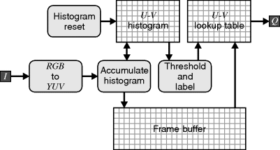
A block diagram for implementing such colour segmentation is shown in Figure 7.25. The scheduling logic is not shown here but effectively controls the sequence as follows:
1. Firstly, the histogram must be initialised by resetting the counts to zero.
2. As the input image is streamed in, it is converted to YUV (or any other convenient colour space). The U and V components are used to increment the corresponding bin in the histogram. The components are also saved in a frame buffer for later classification.
3. Once the histogram is accumulated, the clusters are determined. Here simple thresholding and blob labelling are used, but more sophisticated cluster extraction techniques could be used. The histogram is converted into a lookup table.
4. Finally, the U and V components from the frame buffer are used to index the lookup table to produce the corresponding label for the pixel, producing a streamed output image.
If the labelling is determined offline, then the U and V components may be directly looked up to produce the label. However, the advantage of using the histogram is that the segmentation can be adaptive. The lookup table is also not really required to perform the classification – any of the fixed threshold methods described in Section 6.3.3 could be used, with the data from the histogram used to adapt the threshold levels.
Figure 7.25 Block diagram of a simple colour segmentation scheme.
Once common application of multidimensional histograms is for detecting skin-coloured regions within images (Vezhnevets et al., 2003; Kakumanua et al., 2007). While a number of approaches can be used, histograms may be used to represent the colour distributions of skin and non-skin regions. The initial distributions are established through training, with examples of skin and general background. The histograms, once normalised, give the prior probability of observing a particular colour, I, given the class, ![]() , that is:
, that is:
where ![]() is the histogram for class
is the histogram for class ![]() . Bayes' theorem can be used to invert this to give the probability of a given class given the observed colour:
. Bayes' theorem can be used to invert this to give the probability of a given class given the observed colour:
(7.70) ![]()
where
given that the training samples are provided in the expected proportion of observation and ![]() is the probability of observing a particular colour.
is the probability of observing a particular colour.
The Bayesian classifier then selects the most probable class given the observation, I:
(7.72) 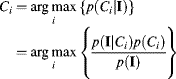
Since the denominator does not depend on i, it will not affect which one is the maximum. Simplifying, and then substituting Equations 7.69 and 7.71 gives:
(7.73) 
Again because the denominator does not depend on i, this may be simplified further:
(7.74) ![]()
In other words, the particular class that has the maximum histogram entry for the observation is the most likely class. Alternatively, if the cost of false positives and false negatives differs, then the histograms may be weighted accordingly before selecting the maximum (Chai and Bouzerdoum, 2000).
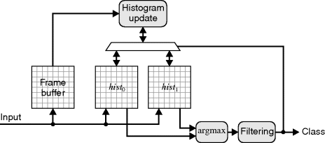
The process can then be made adaptive, by using the classification results to further train the classifier. For this to provide new data, rather than simply to reinforce the existing classification, the output has to be filtered to remove as many misclassifications (both false positives and false negatives) as possible before being fed back. This is shown in block diagram form (without the control logic) in Figure 7.26.
Figure 7.26 Adaptive Bayesian colour segmentation.
Using only the chrominance components will make the colour segmentation independent of the light intensity. However, it has also been shown (Kakumanua et al., 2007) that this will also decrease the discrimination ability, and that better accuracy is obtained with a full three-dimensional colour space.
Toledo et al. (2006) have implemented on an FPGA a histogram-based skin colour detector using a combination of three-dimensional probability maps (histograms) with 32 bins per RGB and YCbCr channel and a combination of two-dimensional histograms using ![]() , and
, and ![]() components. They used a software processor to monitor the results, and adapt the segmentation parameters to improve the tracking performance.
components. They used a software processor to monitor the results, and adapt the segmentation parameters to improve the tracking performance.
7.2.4 Colour Indexing
Histogram similarity, as described in Section 7.1.5, can readily be extended to identification of colour images. This histogram in Equation 7.48 is simply replaced with a multidimensional histogram. The main application of histogram similarity is searching for similar images within an image database. The colour histogram contains much important information that can be used to distinguish different colour images, is invariant to translation and rotation, and is relatively insensitive to the orientation of the object and occlusion. If the colour histogram has a reduced number of bins then the histograms can be much faster to compare than the images themselves. Reasonable results can be achieved with as few as 200 bins (Swain and Ballard, 1991).
One limitation of simple colour indexing is that the search is linear with the size of the database. However, the scaling factor may be improved in a number of ways. The simplest is to reduce the number of bins by combining the counts of groups of adjacent bins. Since:
(7.75) ![]()
the reduced resolution will always give a higher match score than the higher resolution histogram. Therefore, database entries with a low match score may be eliminated at a lower cost.
For many histograms, most of the total count is concentrated in a few bins, corresponding to the dominant colours in the image. The match from these bins has the greatest influence on the match score. An approximate match score may be produced quickly by comparing only those bins with the database histograms. The search speed may be further improved if the database is sorted based on the count in each bin (Swain and Ballard, 1991). This requires a separate database index for each bin, but this index only needs to include those database histograms for which that bin is significant. In this way, large sections of the database that will give a poor match are not even searched. Only those that are likely to give a good match are compared and, even then, only a small number of bins need to be matched. Swain and Ballard (1991) demonstrated that as few as 10 bins actually need to be compared, significantly improving the search time.
If the database contains objects that may be present within the image, then once a match is found, the next step is to locate the actual object within the image. This can be accomplished through histogram back-projection (Swain and Ballard, 1991). The basic idea for this is illustrated in Figure 7.27. Each pixel in the input image is looked up in both the model histogram from the database, ![]() , and the histogram for the image,
, and the histogram for the image, ![]() . The value of the back-projected pixel is then:
. The value of the back-projected pixel is then:
(7.76) ![]()
Figure 7.27 Object location through histogram back-projection.
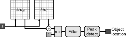
This effectively assigns a high value to the pixels that have a strong colour match with the model, and a low value to the pixels that are not significant in the model. The back-projected image is then smoothed using a suitable filter and the location of the maximum detected. Since the largest peak does not necessarily correspond to the object (sometimes it will be the second or third largest peak), an alternative is to threshold the filtered image to detect candidate locations.
7.2.5 Texture Analysis
Visual texture is characterised by spatial patterns within the pixel values of an image. Since it has a spatial aspect, simple first order statistics are unable to characterise a texture properly. For example, many quite different textures have identical grey-level histograms. It is necessary to capture the spatial relationships using second order statistics. One common method for texture analysis and classification is the based on second order conditional distribution functions, which can be captured in a co-occurrence matrix. This is essentially a two-dimensional histogram, where the first component is the input greyscale image and the second component is the input image offset by distance d in direction ![]() :
:
(7.77) ![]()
where ![]() and
and ![]() . Typically, the city block distance is used and the directions are limited to 45° increments to simplify calculation.
. Typically, the city block distance is used and the directions are limited to 45° increments to simplify calculation.
The spatial grey-level dependence method (SGLDM) (Conners and Harlow, 1980) of texture analysis extracts several features from the co-occurrence matrix. Haralick et al. (1973) define 14, of which five are commonly used (Conners and Harlow, 1980). To obtain meaningful results for comparison or classification, the counts within the two-dimensional histogram must be normalised to give probabilities.
(7.78) 
(7.79) 
(7.80) ![]()
(7.81) 
(7.82) 
where ![]() ,
, ![]() ,
, ![]() , and
, and ![]() are the means and standard deviations of the i and j components respectively of the SGLDM.
are the means and standard deviations of the i and j components respectively of the SGLDM.
Several features are used, over a range of angles, and for a selection of distances that characterise the textures of interest. Some of the features are shown for a sample texture in Figure 7.28, along with the associated SGLDMs displayed as images. The one-dimensional histogram is also shown for reference; it is indistinguishable from a Gaussian distribution and is unable to capture any spatial relationships.
Figure 7.28 A sample texture with its histogram and some associated SGLDM features for ![]() .
.
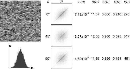
If the whole image contains a single texture, the above analysis is suitable. However, for texture segmentation, the co-occurrence matrices must be calculated from smaller regions or windows within the image. The co-occurrence matrix is more accurate when formed from a large number of pixels. However, for small windows, the measures can become meaningless unless the number of bins in the histogram is reduced accordingly. This has an advantage from an implementation perspective, since the memory required to store the matrix is smaller and calculating the texture features is faster. On an FPGA, the different features may be calculated in parallel as the matrix is scanned. If several matrices are used (with different separations and orientations), the features from these may also be calculated in parallel. Tahir et al. (2003a) do exactly this; they build 16 co-occurrence matrices in parallel with distance ranges of ![]() and angles
and angles ![]() , with 32 pixel value bins in each dimension of their two-dimensional histogram. They also used the FPGA to calculate seven texture features from each matrix in parallel (Tahir et al., 2003b).
, with 32 pixel value bins in each dimension of their two-dimensional histogram. They also used the FPGA to calculate seven texture features from each matrix in parallel (Tahir et al., 2003b).