Chapter 10
Linear Transforms
Linear transformations are often used to rearrange the data into a particular form. In particular they can be used to separate different components of an image, for example separating signal from interference or noise. In general, with a linear transform, each output value is a linear combination of all of the input pixel values:
It extends and generalises local linear filtering of Equation 8.4 by removing the restriction of the window and allowing a more general selection of weights.
Direct implementation of Equation 10.1 is very expensive. If the input image is ![]() , then each output value requires
, then each output value requires ![]() multiplication and additions. For an
multiplication and additions. For an ![]() output, there are therefore
output, there are therefore ![]() operations. Many useful transforms are separable, in that they can be decomposed into separate, independent transforms on the rows and columns. In this case, Equation 10.1 simplifies to:
operations. Many useful transforms are separable, in that they can be decomposed into separate, independent transforms on the rows and columns. In this case, Equation 10.1 simplifies to:
reducing the number of operations to ![]() . Separable transforms can be represented in matrix form as:
. Separable transforms can be represented in matrix form as:
(10.3) ![]()
where w, I, and Q are the weights and two-dimensional input and output images represented directly as matrices. All of the transforms considered in this chapter are separable, so only the detailed implementation of the one-dimensional transform will be considered. To implement the two dimensional transform, the architectures of Figures 9.5 and 9.6 can be used.
In many cases, the transform matrix, w, may be further factorised into a cascade of simpler operations. Such factorisations allow so-called fast transforms reducing the number of operations to order ![]() .
.
If the rows of w are orthogonal and normalised so that the length is one:
(10.4) ![]()
then the transformation matrix is unitary and the transformation can be considered in terms of projecting the input image onto a new set of coordinate axes. The new axes may be thought of as basis images or component images, with the transformed values indicating how much of each basis image, ![]() , is in the original image. Thus:
, is in the original image. Thus:
In this context, Equation 10.1 is sometimes called the analysis equation, because it is analysing how much of each basis image is present, and Equation 10.5 is called the synthesis equation, because it is synthesising the image from the basis images.
The Fourier transform is one of the most commonly used linear transforms in image and signal processing. It transforms the input image from a function of position ![]() to a function of spatial frequency
to a function of spatial frequency ![]() in the frequency domain:
in the frequency domain:
(10.6) 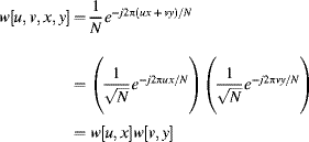
The factor of ![]() is often left out of the forward transform and
is often left out of the forward transform and ![]() is applied to the inverse transform. The Fourier transform is clearly separable, and is complex valued in the frequency domain. The periodic nature of the basis functions implies that the image is periodic in both space and frequency. That is:
is applied to the inverse transform. The Fourier transform is clearly separable, and is complex valued in the frequency domain. The periodic nature of the basis functions implies that the image is periodic in both space and frequency. That is:
This is a consequence of both the image and frequency domains being sampled (Bracewell, 2000). Although the origin in the frequency domain (corresponding to DC) is in the corner of the image, it is often shifted to the centre for display purposes by scrolling the image by ![]() pixels both horizontally and vertically. Equation 10.7 also implies that the Fourier transform of a real image is conjugate symmetric.
pixels both horizontally and vertically. Equation 10.7 also implies that the Fourier transform of a real image is conjugate symmetric.
Two example images and their Fourier transforms are shown in Figure 10.1. On the top is a sinusoidal intensity pattern. Its Fourier transform has three peaks, one for the DC or average pixel value, and one for each of the positive and negative frequency components. This symmetry results from the Euler identity:
(10.8) 
Figure 10.1 Example Fourier transforms: Top: sinusoid; bottom: semi-regular pattern, the magnitude in the frequency domain has been logarithmically transformed to show the detail more clearly.
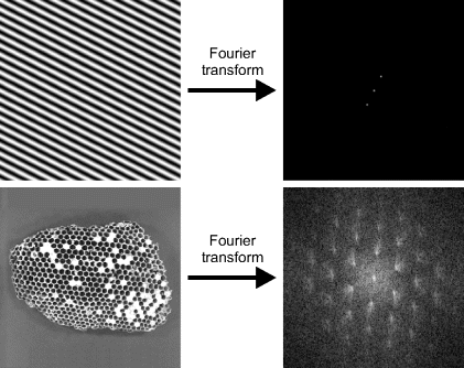
In general, an image with a periodic spatial pattern will have a set of peaks in the frequency domain, corresponding to the frequency of the pattern along with its harmonics (Bailey, 1993; 1997b). The position of a peak in the frequency domain indicates the spatial frequency of the corresponding pattern in the image, with the frequency proportional to the distance from the origin and the direction of the peak from the origin corresponding to the direction of the sinusoidal variation. Rotating an object spatially will result in its Fourier transform rotating by the same angle. The magnitude of the peaks corresponds to the amplitude of the pattern, and the phase of the frequency components contains information about the position of the pattern in the image (shifting an object will only change the phase of the corresponding frequency terms, not their amplitude). The shape of the peaks contains information about the shape and size of patterns in the image, and the distribution of the peaks relates to the details of the object. For example, sharp edges within the pattern will result in harmonics with amplitudes that drop in inverse proportion with frequency. In general, the amplitude of natural images in the frequency domain drops approximately in inverse proportion with frequency, primarily as a result of edges and other discontinuities within the images (Millane et al., 2003). In contrast to this, spatially uncorrelated random noise has a uniform frequency distribution.
Some imaging modalities (for example magnetic resonance imaging and X-ray crystallography) capture their data in the frequency domain and it must be converted to the spatial domain for visualisation. In other applications, the desired image processing operation may be simpler to perform in the frequency domain, requiring the use of a forward and inverse Fourier transform to switch between the spatial and frequency domains.
10.1.1 Fast Fourier Transform
A fast Fourier transform (FFT) is an efficient implementation of the Fourier transform that results from the factorisation of the transformation. First define:
(10.9) ![]()
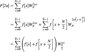
Then, by splitting the input into the odd and even samples:
(10.10) ![]()
the Fourier transform can be expanded as a sum of the Fourier transforms of the odd and even samples:
(10.11) 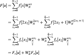
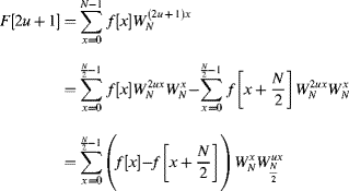
A further simplification may be arrived at by considering periodicity and symmetry. Since the Fourier transform is periodic, ![]() and by symmetry
and by symmetry ![]() . Therefore, the second half of the frequency samples become:
. Therefore, the second half of the frequency samples become:
(10.12) 
which reuses the Fourier transforms of the first half, but with a change in sign. The ![]() factors are sometimes called twiddle factors. By recursively applying this same decomposition to
factors are sometimes called twiddle factors. By recursively applying this same decomposition to ![]() and
and ![]() , the
, the ![]() levels of the radix-2 decimation in time fast Fourier transform results. This is illustrated for
levels of the radix-2 decimation in time fast Fourier transform results. This is illustrated for ![]() in Figure 10.2. The computation at each level is split into a series of ‘butterfly’ computations, which can be performed in place in a memory-based system.
in Figure 10.2. The computation at each level is split into a series of ‘butterfly’ computations, which can be performed in place in a memory-based system.
Figure 10.2 Radix-2 decimation in time FFT. Right: basic butterfly operation.
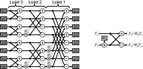
The limitation of the decimation in time decomposition is that the input samples are in a bit-reversed order if applied in place. The operations can be rearranged so that the input operations are sequential, in which case the outputs are in a bit-reversed order.
An alternative decomposition is decimation in frequency. Calculating the even and even frequency components separately gives:
and
These are Fourier transforms of sequences which have half the length of the original sequence. Repeating this recursively gives the decimation in frequency algorithm illustrated in Figure 10.3. The input samples are ordered naturally, and the frequency samples use bit-reversed addressing as a consequence of separating the outputs in terms of odd and even components. The main differences in the calculation are the order of the groupings and that the twiddle factor is on the output of the butterfly rather than the input.
Figure 10.3 Radix-2 decimation in frequency FFT. Right: basic butterfly operation.
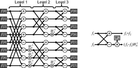
In many applications, the scrambling of the frequency samples is of little consequence. If an FFT is followed by a point operation in the frequency domain and then an inverse FFT, the frequency scrambling is of no consequence. Alternatively, if the transform is not performed in place, but goes from one memory to another, then the order of the samples may be rearranged during the process.
Note that all of the operations illustrated in Figures 10.2 and 10.3 are on complex numbers. In particular, each complex multiplication requires four real multiplications and two additions. However, through factorisation, the number of multiplications can be reduced to three at the cost of three more additions:
Within the FFT, two of these additions are between constants, effectively trading one multiplication for an addition (see Figure 10.8).
Since each multiplication is effectively a rotation in the complex plane (![]() ), the complete multiplication can be performed efficiently using CORDIC arithmetic (Despain, 1974; Sansaloni et al., 2003). Efficiencies can be gained because the rotation angles are constants, so the decisions at each step of the CORDIC algorithm may be made in advance rather than having to wait for the signal to propagate through to the sign bit (the
), the complete multiplication can be performed efficiently using CORDIC arithmetic (Despain, 1974; Sansaloni et al., 2003). Efficiencies can be gained because the rotation angles are constants, so the decisions at each step of the CORDIC algorithm may be made in advance rather than having to wait for the signal to propagate through to the sign bit (the ![]() register and logic are also eliminated, Section 5.4.3). However, compensated CORDIC is required to prevent the magnitude from changing as the complex number is rotated.
register and logic are also eliminated, Section 5.4.3). However, compensated CORDIC is required to prevent the magnitude from changing as the complex number is rotated.
While the radix-2 algorithms (decomposing the transformation to a series of two point Fourier transforms) are the simplest to understand, the number of multiplications may be reduced by using a radix-4 algorithm. A four-point Fourier transform is:
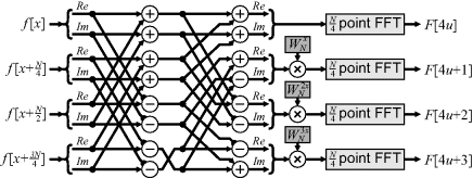
and the multiplication by j is trivial. The radix-4 decimation in frequency algorithm extends Equations 10.13 and 10.14 by splitting the input into four Sections, combining them using Equation 10.16 and taking the ![]() -point transforms of the results to get the frequency samples decimated by four:
-point transforms of the results to get the frequency samples decimated by four:
(10.17) 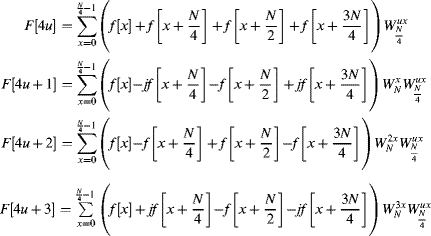
The corresponding ‘butterfly’ is shown in Figure 10.4. Although such decimation can be extended to higher radixes, little is gained beyond radix-4.
Figure 10.4 Radix-4 decimation in frequency butterfly with the real and imaginary components shown explicitly.
There are several ways in which the FFT may be implemented given the above building blocks. If resources are scarce, a single butterfly unit may be built, with the transformation performed in place in memory (Figure 10.5). The data is first streamed into memory (performing any permutation as necessary). The data is then accessed from memory as needed for each butterfly operation, with the results written back into memory. Bandwidth limitations limit the speed to one butterfly every two clock cycles for the radix-2 and one butterfly every four clock cycles for the radix-4 operation. With the radix-4 butterfly, the multiplier can be shared by moving it from within the butterfly to after the multiplexer, as shown in Figure 10.5 (Sansaloni et al., 2003). With the radix-4 butterfly, the number of adders may also be reduced by multiplexing the input layer of Figure 10.4. The throughput (and latency) may be improved by splitting the memory into multiple blocks (two for radix-2 and four for radix-4) to enable one operation to be performed every clock cycle. The memory addressing becomes considerably more complex because to ensure that the data will be available when it is needed, the transformation cannot be performed in place.
Figure 10.5 FFT with a single butterfly. Left: radix-2; right: radix-4 FFT.

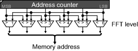
The memory addressing required by the scheme in Figure 10.5 is relatively straightforward. A standard counter may be used, with the address bits permuted depending on the FFT level. The read address for the radix-2 decimation in frequency FFT is shown in Figure 10.6. The write counter is the same, only delayed by a few clock cycles depending on the latency of the butterfly and associated registers. The address counters are similar for the other FFT implementations based on sharing a single butterfly.
Figure 10.6 Memory read address counter for radix-2 decimation in frequency FFT.
Uzun et al. (2003; 2008) implemented several different butterfly implementations within a generic framework using Handel-C. The speed and resources were compared between the implementations for a number of butterfly units. Not surprisingly, the radix-4 algorithm was the fastest, but also consumed the most resources.
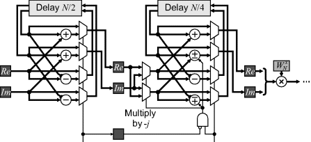
If more resources are available, multiple butterflies may be implemented and the FFT pipelined to increase the throughput. A range of radix-2 and radix-4 pipelined FFT approaches have been reviewed by He and Torkelson (1996). One of the more efficient pipelined implementations is the radix-22 scheme illustrated in Figure 10.7. This uses a radix-2 butterfly with the stages in pairs effectively forming a radix-4 transform. It retains the simplicity of the reduced number of multipliers as the radix-4 algorithm, with a single complex multiplier only required after every second stage. At each stage, the first half of the clock cycles feed the data through into the delay register without processing. The second half combines the incoming data with the delayed data, performing the butterfly. One of the butterfly outputs is fed directly out to the next stage, while the other is fed back into the delay. It is finally output while the next block is being loaded. Successive stages reduce the delay by a factor of two to give the interleaving as illustrated in Figure 10.3. Control consists of the successive bits of a binary counter (delayed as necessary to account for any pipeline delays). The pipelined FFT takes streamed data as input and produces a streamed output (in bit-reversed order). The throughput of these arrangements is one clock cycle per sample, with a latency of one row. FPGA-based implementations of this scheme have been described by Sukhsawas and Benkrid (2004) and Saeed et al. (2009).
Figure 10.7 Pipelined radix-22 implementation. Shown are the first two stages. This structure is repeated with successive stages alternating.
To perform an inverse FFT, the inverse transform matrix is the complex conjugate of the forward transform. This means that the same hardware may be used, with the exception that the complex conjugate of the twiddle factors is used. Alternatively, the inverse FFT may be calculated by taking the complex conjugate of the frequency domain signal and using a standard forward FFT. With either case the result needs to be divided by N to obtain the original signal.
While an FFT is mathematically invertible, with inevitable round-off errors in twiddle factors and truncating the results of the multiplication this mean that the result is only an approximation of the Fourier transform. Consequently, taking the FFT and then the inverse FFT will not necessarily give exactly the same result. The transform may be made invertible by using a lifting scheme to implement the twiddle factor multiplications (Oraintara et al., 2002). The lifting scheme is compared with conventional complex multiplication and the factorised multiplication of Equation 10.15 in Figure 10.8. The two alternatives for the lifting scheme enable the absolute value of the coefficients to be kept less than one (the final multiplication is a trivial sign change). One disadvantage of using the lifting scheme is that the multiplications are performed in series rather than in parallel as with the other two methods, increasing the latency.
Figure 10.8 Complex multiplication. Left: conventional multiplication; centre: factorised implementation using Equation 10.15; right: implemented using a lifting scheme.

Although the lifting scheme still suffers from round-off and truncation errors, the errors are reversible if the result of the multiplication is quantised before the associated addition. Running the system in reverse, replacing the additions with subtractions, will give the original result provided that an identical quantisation is performed.
To calculate the FFT of a two-dimensional image the Fourier transform can be taken of each of the rows, and then of the columns of the result. Since each of the row transforms is of independent data, the two-dimensional transform may be accelerated by performing multiple row transforms in parallel through hardware duplication. Similarly, the column transforms may also be performed in parallel.
With real data, additional efficiencies may be gained by performing two FFTs at once. The Fourier transform of a real signal is conjugate symmetric, that is the real parts of the Fourier transform are even and the imaginary parts are odd. This allows a single FFT to take the Fourier transform of two sequences simultaneously. Let two separate rows be ![]() and
and ![]() . A composite signal is formed by combining one signal in the real part and the other in the imaginary:
. A composite signal is formed by combining one signal in the real part and the other in the imaginary:
The FFT is taken of the composite signal and the FFT of the individual components may be extracted as:
This is effectively another level of butterfly operations, although with a different pattern. Similarly, when performing the inverse FFT of a real image, two conjugate symmetric Fourier transforms may be combined as:
before calculating the inverse.
When calculating the Fourier transform of a two-dimensional image, symmetry may also be exploited when taking the Fourier transform of the columns. Columns 0 and ![]() will only have real data, so may be transformed together with a single FFT. Columns u and
will only have real data, so may be transformed together with a single FFT. Columns u and ![]() will be complex conjugates of one another, so will give related Fourier transforms:
will be complex conjugates of one another, so will give related Fourier transforms:
(10.21) ![]()
Therefore, only one of these needs to be calculated. Exploiting the symmetries of both row and column transforms reduces the overall computation for the two-dimensional FFT of a real image by a factor of four.
When performing a two-dimensional FFT, a one-dimensional FFT must be performed on all of the rows (or columns) before repeating the FFT in the other direction. This requires storing the frequency domain image into a frame buffer before performing the column FFTs. Processing a streamed input, and assuming that only half of the frequency domain needs to be calculated, the latency of performing a two-dimensional FFT is approximately one half of a frame time (from the time the last pixel is input to when the last pixel is output). Many operations (filtering for example) require only a point operation in the frequency domain. Therefore, taking the inverse FFT of the columns can be pipelined with the forward FFT. Again, all of the columns must be completed before taking the inverse FFT of the rows. Using Equation 10.20 to take the inverse of two rows at once will give an overall latency of frequency domain processing of just over one frame time.
The assumption throughout this Section has been that N is a power of two. While other factorisations of N can also result in fast algorithms, they lack the elegance and computational simplicity of those described above for powers of two. Therefore, unless there is a particular need for a special size, the complexity of developing the circuitry for such factorisations is generally not worthwhile. An alternative is to express the Fourier transform in terms of a convolution, which can be calculated using a power of two FFT (Bergland, 1969). In one dimension:
(10.22) 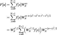
The summation is now a convolution, which may be performed by using an FFT of length ![]() of each of the two sequences, taking their product and calculating the inverse FFT of the result. While this requires calculating three longer FFTs, in many circumstances this is still preferable to calculating the Fourier transform directly (especially if N is prime and cannot be factorised).
of each of the two sequences, taking their product and calculating the inverse FFT of the result. While this requires calculating three longer FFTs, in many circumstances this is still preferable to calculating the Fourier transform directly (especially if N is prime and cannot be factorised).
10.1.2 Filtering
Linear filters are implemented as a convolution in the image domain, using Equation 8.4. In the frequency domain, this convolution becomes a product:
where ![]() is the Fourier transform of the flipped filter kernel. Filtering may therefore be performed in the frequency domain. For large kernel sizes, it is less expensive computationally to take the Fourier transform (using an FFT), multiply by
is the Fourier transform of the flipped filter kernel. Filtering may therefore be performed in the frequency domain. For large kernel sizes, it is less expensive computationally to take the Fourier transform (using an FFT), multiply by ![]() and take the inverse Fourier transform of the result.
and take the inverse Fourier transform of the result.
The weighting in the frequency domain of Equation 10.23 implies that a linear filter may, therefore, be considered in terms of its frequency response, as a weighting of the different frequency components within the image. In this context, a low pass filter will tend to smooth noise, because it will pass low frequencies with little attenuation, and many images have most of their energy in the low frequency. Uncorrelated noise has uniform frequency content, so attenuating the high frequencies will have only a small effect on the image, but a more significant effect on the noise. The loss of high frequencies in the image will result in a loss of fine detail which will, in general, blur the image. Edges and fine detail may be enhanced by boosting the amplitudes of the higher frequencies, but this will also tend to amplify the noise within the image.
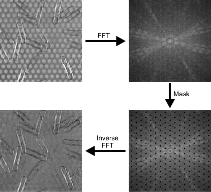
One particular application of filtering in the frequency domain is to remove pattern noise from an image. As described earlier, a regular pattern will exhibit a series of peaks within the frequency domain. These peaks may be detected directly in the frequency domain and masked out, as demonstrated in Figure 10.9. If the pattern is added within the image, then filtering can remove the pattern. Here the pattern is part of the background, so removing the pattern will also affect the object itself.
Figure 10.9 Filtering to remove pattern noise. The frequency domain is shown logarithmically scaled for clarity.
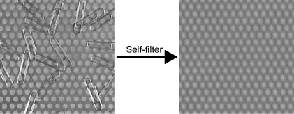
The opposite of removing pattern noise is filtering to detect regular patterns within the image. In this case, it is the periodic peaks within the frequency domain that contain the information of interest. One approach to enhancing the regular patterns is to use the image itself as the filter (Bailey, 1993; 1997b). Multiplication by the magnitude in the frequency domain:
is a zero phase filter, so objects are not shifted. Self-filtering is demonstrated in Figure 10.10. The basic self-filter will blur sharp edges, which have frequency content that rolls off inversely proportional to frequency. This may be compensated by weighting the filter with frequency to reduce the attenuation of the harmonics:
(10.25) ![]()
Figure 10.10 Self-filtering in the frequency domain using Equation 10.24.
In the example in Figure 10.9, the frequency domain was simply masked. This will also remove those frequency components from the objects of interest. An alternative is to design the filter such that it minimises the error after filtering. Consider an image, ![]() , which has been corrupted by the addition of noise,
, which has been corrupted by the addition of noise, ![]() (uncorrelated with the input image). The Wiener filter is the optimal filter (in the least squares sense) for recovering the original signal. The analysis is easiest to perform in the frequency domain: the goal is to determine the filter
(uncorrelated with the input image). The Wiener filter is the optimal filter (in the least squares sense) for recovering the original signal. The analysis is easiest to perform in the frequency domain: the goal is to determine the filter ![]() that minimises the error:
that minimises the error:
(10.26) 
This can be simplified by making the assumption that the filter is symmetric so that it does not shift the image. Therefore, W is real, resulting in:
(10.27) ![]()
The expected value of the second summation is zero if the image and signal are uncorrelated. Therefore:
(10.28) ![]()
The error may be minimised by taking the derivative with respect to the filter:
(10.29) ![]()
The corresponding optimal filter is, therefore:
Given estimates of both the signal and noise spectra, the frequency response of the optimal filter can be derived. If the noise is uncorrelated, then it will have a flat spectrum and will be a constant.
Equation 10.30 may be interpreted as follows: at the frequencies where the signal is much larger than the noise, the frequency response of the filter will approach unity, passing the signal through. However, the frequencies at which the signal is smaller than the noise will be attenuated, effectively reducing the noise power while having little effect on the total signal. The Wiener filter is effective are removing both random noise as well as pattern noise.
10.1.3 Inverse Filtering
Closely related to filtering is inverse filtering. Here the goal is to remove the effects of filtering from an image. A common application is removing blur, whether from the lens point spread function, or motion blur from a moving object or camera. Let ![]() be the blur point spread function, with corresponding Fourier transform,
be the blur point spread function, with corresponding Fourier transform, ![]() . Also, let the desired unblurred image be
. Also, let the desired unblurred image be ![]() . In the frequency domain the blurred image is given by:
. In the frequency domain the blurred image is given by:
(10.31) ![]()
Assuming that the blur function is known, then the deblurred image should be able to be recovered as:
Unfortunately, this does not work. The output image from Equation 10.32 appears to contain only random noise. The reason is that ![]() goes to zero at some frequencies. This division by zero is undefined. Even if B does not actually go to zero at any of the samples, the scaling of the corresponding frequencies becomes arbitrarily large. For noiseless, infinite precision arithmetic, this would not pose a problem. However,
goes to zero at some frequencies. This division by zero is undefined. Even if B does not actually go to zero at any of the samples, the scaling of the corresponding frequencies becomes arbitrarily large. For noiseless, infinite precision arithmetic, this would not pose a problem. However, ![]() will inevitably have some level of noise added. Applying the inverse filter according to Equation 10.32 will cause the noise to dominate the output.
will inevitably have some level of noise added. Applying the inverse filter according to Equation 10.32 will cause the noise to dominate the output.
One solution to this problem is to manipulate Equation 10.32 to avoid division by zero:
(10.33) ![]()
where the first transformation is to make the denominator positive real and the second adds a positive constant, ![]() , in the denominator to prevent division by zero. This effectively limits the gain of the noise. The Wiener filter, which minimises the mean square error, gives the inverse filter as:
, in the denominator to prevent division by zero. This effectively limits the gain of the noise. The Wiener filter, which minimises the mean square error, gives the inverse filter as:
(10.34) 
which sets ![]() optimally according to the signal-to-noise ratio at each frequency.
optimally according to the signal-to-noise ratio at each frequency.
More complex techniques (usually iterative) are required when the blur function is not known. These are beyond the scope of this book.
10.1.4 Interpolation
Images may be interpolated by using the frequency domain. If it is assumed that the image is band-limited (and sampled according to the Nyquist sampling criterion), then extending the image in the frequency domain is trivial because the additional higher frequency samples will be zero. Therefore, an image may be interpolated by taking its Fourier transform, padding with zeros and taking the inverse Fourier transform.
Since padding will make the frequency domain image larger, taking the inverse Fourier transform will take longer. This approach is equivalent to sinc interpolation of the input image. However, in many imaging applications, the input image is not band-limited, therefore sinc interpolation will not necessarily give the best results. Interpolating directly in the image domain (Section 9.3) is usually more appropriate.
If multiple, slightly offset, images are available, then a simple approach to image super-resolution is to use the information gleaned from the multiple images to resolve the aliasing, giving an increased resolution (Tsai and Huang, 1984). As a result of aliasing, the value at each frequency sample will result from a mixture of frequencies:
(10.35) ![]()
where ![]() are the samples of the continuous frequency distribution of the original unsampled image. Normally, once the frequency information has been aliased, it is impossible to distinguish between the different frequency components that have been added together. However, when an image is offset, the different aliased components will have a different phase shift (since the phase shift is proportional to frequency). Therefore, given multiple offset images, it is possible to untangle the aliasing. Consider enhancing the resolution by a factor of two. Then each image may be considered as:
are the samples of the continuous frequency distribution of the original unsampled image. Normally, once the frequency information has been aliased, it is impossible to distinguish between the different frequency components that have been added together. However, when an image is offset, the different aliased components will have a different phase shift (since the phase shift is proportional to frequency). Therefore, given multiple offset images, it is possible to untangle the aliasing. Consider enhancing the resolution by a factor of two. Then each image may be considered as:
(10.36) ![]()
where it is assumed that the additional higher order alias terms are negligible. The phase terms are determined directly from the offsets of each of the images (for example, using any of the techniques of Section 9.5) and are effectively known (or can be estimated). Given four such images, then in matrix form:
(10.37) 
This equation may be inverted to resolve the aliased higher frequency components. (If more images are available, a least squares inverse may be used to improve the estimate.) By padding the image with these components and taking the inverse Fourier transform, the resolution may be improved.
10.1.5 Registration
As outlined in the previous chapter, images may be registered in the frequency domain. This requires taking the Fourier transform of the two input images being registered. Using Equations 10.18 and 10.19, these may be calculated in parallel using a single FFT. CORDIC arithmetic can then be used to obtain the magnitude and phase angle of each frequency component. To estimate the offset, it is necessary to determine the slope of the phase difference. The problem here is that the arctangent reduces the phase to within ![]() , requiring the phase to be unwrapped.
, requiring the phase to be unwrapped.
In many applications it can be assumed that the phase varies slowly with frequency. The simplest approach to phase unwrapping is to consider the phase of adjacent samples. Multiples of ![]() are then added to one of the samples until the absolute difference is less than
are then added to one of the samples until the absolute difference is less than ![]() . In two dimensions, this may be applied both horizontally and vertically, providing additional constraints.
. In two dimensions, this may be applied both horizontally and vertically, providing additional constraints.
One limitation with this approach is that, at some frequencies, the amplitude changes sign (consider for example a sinc function). The phase shift between such points should be close to ![]() rather than zero. A second limitation is that when the magnitude is low, the phase angle becomes dominated by noise. Consequently, only the phases for the low frequencies are reliably unwrapped unless more complex methods are used.
rather than zero. A second limitation is that when the magnitude is low, the phase angle becomes dominated by noise. Consequently, only the phases for the low frequencies are reliably unwrapped unless more complex methods are used.
In the case of image registration, the phase difference should be planar. One approach to this is to fit a plane to the phase difference. An alternative is to consider the phase shear (Stowers et al., 2010). From Equation 9.51:
(10.38) ![]()
Let ![]() . Then the phase difference between horizontally adjacent frequencies should be:
. Then the phase difference between horizontally adjacent frequencies should be:
An amplitude weighted average of these is given by (Stowers et al., 2010):
(10.40) ![]()
and similarly for the vertical offset. The amplitude weighting will automatically give low weight to those differences where the phase shifts by ![]() , and the problem of phase wrapping is avoided by deferring the arctangent to after the averaging.
, and the problem of phase wrapping is avoided by deferring the arctangent to after the averaging.
Alternatively, histograms of the horizontal and vertical offsets estimated by Equation 10.39 may be built to enable outliers to be eliminated before averaging.
10.1.6 Feature Extraction
The frequency domain can provide a rich source of features, particularly in representing the texture within an image. The example in Figure 10.11 shows an electron micrograph of the surface of a pollen grain. From the frequency domain, the dominant frequency and angle variation may be easily measured (Currie, 1995).
Figure 10.11 Frequency domain features: dominant frequency and angle distribution. Top: taking the Fourier transform directly of the image; bottom: windowing the image first.
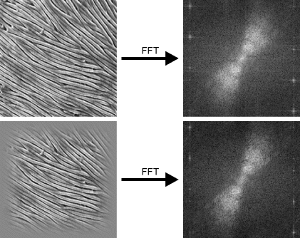
The top row of Figure 10.11 shows one of the limitations of using the discrete Fourier transform (calculated via the FFT). Sampling in the frequency domain implicitly assumes that the image is periodic. However, the pattern on the left and right edges of the image do not line up. These discontinuities result in spectral leakage, the manifestation of which is the streaked appearance within the frequency domain.
Spectral leakage effects may be reduced by multiplying the input image by a window or apodization function, which smoothly tapers to zero at the edges of the image:
(10.41) ![]()
This product becomes a convolution of Fourier transforms, so the default rectangular window will convolve the true frequency content with a sinc function. It is the relatively high sidelobes of the sinc function that results in spectral leakage, and the streaking and smearing in the frequency domain. The consequences of using a windowing function are a reduction in the level of the sidelobes at the expense of an increased main lobe. The reduction in side lobes directly reduces the spectral leakage, but the wider main lobe results in reduced frequency resolution from the blurring within the frequency domain (Harris, 1978).
The window function in the lower image in Figure 10.11 was a Tukey or tapered cosine window with ![]() :
:
(10.42) 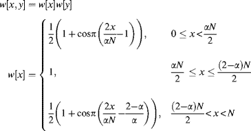
This window provides a compromise between maintaining good frequency resolution while reducing spectral leakage.
For an FPGA implementation, the window function may be stored in a lookup table, and multiplied by the incoming image as the first step before calculating the FFT. Due to symmetry, only ![]() entries are required in the table. For the 25% Tukey window, this is reduced to
entries are required in the table. For the 25% Tukey window, this is reduced to ![]() entries.
entries.
10.1.7 Goertzel's Algorithm
In some applications, only one or a few frequencies are of interest. In this case, Goertzel's algorithm (Goertzel, 1958) can require considerably fewer calculations than performing the full Fourier transform. Consider a single frequency component of the Fourier transform:
(10.43) 
This is effectively a recursive calculation:
(10.44) ![]()
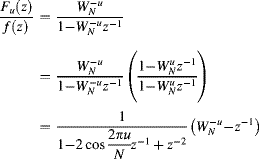
It still requires one complex multiplication per sample, so does not gain anything computationally. Looking at this recursion in the z-domain:
The multiplication of the top and bottom by the complex conjugate of the denominator makes the denominator coefficients real. Therefore, the first term can be implemented as a second order recursion with real coefficients:
(10.46) ![]()
and after the ![]() samples have accumulated, the frequency term may be calculated from the second term of Equation 10.45 as:
samples have accumulated, the frequency term may be calculated from the second term of Equation 10.45 as:
(10.47) ![]()
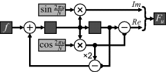
An implementation of this is shown in Figure 10.12. Note that the intermediate registers need to be reset to zero before the start of the calculation. The filter processes streamed data and produces the frequency value after ![]() input samples.
input samples. ![]() is not restricted to a power of two – the implementation of the algorithm is independent of the number of samples (apart from the constant multipliers). If multiple frequencies must be calculated, then this circuit can be duplicated for each frequency.
is not restricted to a power of two – the implementation of the algorithm is independent of the number of samples (apart from the constant multipliers). If multiple frequencies must be calculated, then this circuit can be duplicated for each frequency.
Figure 10.12 Implementation of Goertzel's algorithm.
10.2 Discrete Cosine Transform
Closely related to the Fourier transform is the discrete cosine transform (DCT). Whereas the Fourier transform has both sine and cosine components, the DCT is made purely from cosine terms. This is achieved by enforcing even symmetry and enables the transform to be calculated with real rather than complex numbers.
Mathematically, in one dimension the discrete cosine transform is:
(10.48) 
or in terms of Equation 10.2:
(10.49) 
The inverse is simply ![]() or:
or:
(10.50) 
Being separable, a two-dimensional DCT may be calculated by taking the one-dimensional transform of the rows followed by the one-dimensional transform of the columns. While algorithms for direct computation of the two-dimensional transform can be developed that require fewer arithmetic operations than the separable transform (Feig and Winograd, 1992), the separable algorithm allows hardware to be reused and results in a simpler implementation for streamed data.
Since it is closely related to the Fourier transform, there are also fast algorithms for calculating the DCT, especially for powers of two. In fact, the DCT can be calculated using an FFT of length ![]() , with the data in the odd terms (mirroring the data to maintain even symmetry) and setting the even terms to zero. The appropriate simplifications of the resulting FFT (removing unnecessary calculations) lead to efficient algorithms for the DCT. Algorithms are discussed here for
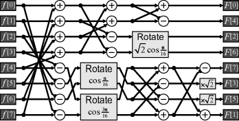
, with the data in the odd terms (mirroring the data to maintain even symmetry) and setting the even terms to zero. The appropriate simplifications of the resulting FFT (removing unnecessary calculations) lead to efficient algorithms for the DCT. Algorithms are discussed here for ![]() , since this is the size most commonly used for image and video coding. The most efficient algorithm for an eight-point DCT requires 11 multiplications (Loeffler et al., 1989) and is shown in Figure 10.13.
, since this is the size most commonly used for image and video coding. The most efficient algorithm for an eight-point DCT requires 11 multiplications (Loeffler et al., 1989) and is shown in Figure 10.13.
Figure 10.13 DCT with 11 multiplications. The Rotate box is a scaled rotation requiring three multiplications and additions using Equation 10.15.
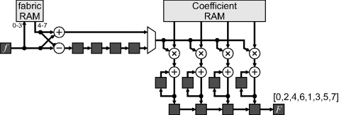
If a scaled DCT is acceptable, the number of multiplications can be reduced to five (Kovac and Ranganathan, 1995) (Figure 10.14). With a scaled DCT, each frequency coefficient is scaled by an arbitrary factor. When using the DCT for image compression, the coefficients are quantised. The scale factor can be incorporated into the quantisation step without incurring any additional operations simply by scaling the quantisation step size by scale factor. Agostini et al. (2001; 2005) have implemented this on an FPGA for JPEG image compression. Their implementation had a throughput of one pixel per clock cycle but with a latency of 48 clock cycles because they divided the algorithm into six blocks to share hardware. The structure of the DCT is less regular than the FFT, making an elegant pipeline less practical. However, one attempt at pipelining the scheme of Figure 10.14 is shown in Figure 10.15. Attempts have been made to reuse hardware where practical, particularly the multiplier. This design maintains a throughput of one pixel per clock cycle and has a latency of only nine clock cycles.
Figure 10.14 Scaled DCT (Kovac and Ranganathan, 1995), where ![]() . The fixed multipliers are
. The fixed multipliers are ![]() ,
, ![]() ,
, ![]() ,
, ![]() .
.
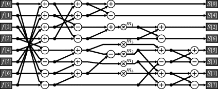
Figure 10.15 A pipelined implementation of Figure 10.14. Numbers on registers and multiplexers refer to the clock cycle they are active relative to the input samples entering on clocks 0 to 7. The registers should be clocked and the corresponding multiplexer inputs selected on these cycles.

The first four samples are stored in a fabric RAM and are read out in the next four samples to be combined with the input. Using a RAM reduces the need for explicit multiplexing. Similarly, the constant multipliers can also be stored in a fabric RAM, to enable sequential access. The assumption made here is that the multiplication can be completed in a single clock cycle. If not, the multiplier will need to be pipelined and additional delays inserted in the corresponding parallel paths. The scaled outputs are not in natural order; for JPEG compression, this does not matter because the data will be reordered later using a zigzag buffer.
Modern FPGAs have plentiful multipliers. This enables a far simpler and more elegant pipelined design, as demonstrated in Figure 10.16. It simply multiplies the incoming pixel values by the appropriate DCT matrix coefficients and accumulates the results (Woods et al., 1998). One level of factorisation is used to reduce the number of multiplications from eight to four. Each multiply and accumulate unit is reset every four clock cycles and calculates a separate output frequency. The factorisation means that the even and odd samples are calculated separately.
Figure 10.16 Using parallel multipliers to perform an eight-point DCT.
With block processing, all published systems operate on a block at a time. That is they process each of the rows of a block, saving the results into a transpose buffer, and then use a second processor take the DCT of the columns, as illustrated in Figure 10.17. The transpose buffer can be readily implemented using a dual-port block RAM. One port is used to write the results of the row transform, while the second port is used to read the values in column order. The block RAM in most FPGAs is also sufficiently large to hold two blocks of data, enabling bank switching to be incorporated directly within the single memory simply by controlling the most significant address bit.
Figure 10.17 Two-dimensional discrete cosine transform of a block.

An alternative approach with data streamed from the camera is to calculate the row DCTs as the data is streamed from the camera, storing the intermediate results in an on-chip cache. Once the eighth row arrives, the data may be read from the cache in column order to perform the column DCTs. With either approach, the cache needs to hold 14 rows of data (effectively seven row buffers for each of the row and column transforms). With the latter approach, a transpose buffer is not required, but the cache may need to be a few bits wider to match the required precision of the intermediate result.
Similar circuits may be used for calculating the inverse DCT. Since the inverse uses the transposed coefficient matrix, similar factorisations to the forward transform may also be used.
The application of the DCT to image and video coding is discussed in more detail in Section 10.4.
One of the limitations of frequency domain transformations, such as the Fourier transform and cosine transform, is that the resolution in the frequency domain is inversely proportional to that in the image domain. This is illustrated in one dimension in Figure 10.18. Features which are narrow in space have a wide frequency bandwidth, and a narrow frequency (for example, a sine wave) has a wide spatial extent.
Figure 10.18 Trade-off between spatial and frequency resolution, illustrated in one dimension. Left: image samples; centre: frequency samples from Fourier transform; right: trade-off from the wavelet transform.

One implication of this is that to obtain good frequency resolution, it is necessary to have a large number of samples in the image. Increasing the frequency resolution requires extending the width of the image. However, in taking the Fourier transform, the direct location of features and objects within the image is lost. Good spatial resolution of an object requires looking within a narrow window within the image, which results in poor frequency resolution.
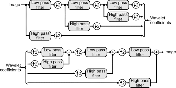
At low frequencies, the spatial resolution is inevitably poor anyway because of the long period. However, the shorter periods of high frequencies makes higher spatial resolution more desirable. This is achieved by dividing the position–frequency space as shown in the right hand panel of Figure 10.18. This is achieved by wavelet analysis as follows. Firstly, the image is filtered, separating the low and high frequency components. As a result of the reduction in bandwidth, these components can be down-sampled by a factor of two by discarding every second sample. This gives the position–frequency resolution aspect ratio seen in the figure for the high frequency components. This process is then recursively repeated on the low frequency components giving the desired position–frequency resolution. The schematic of this process in one dimension is given in Figure 10.19. The wavelet transform effectively looks at the image at a range of scales. For each level of the wavelet transform, the low pass filter outputs are often called the approximation components, whereas the high pass filter outputs are the detail components.
Figure 10.19 Wavelet transform in one dimension, with three decomposition levels shown. Top: wavelet analysis or decomposition; bottom: reconstruction of the original signal, or synthesis.
With the Fourier transform, every frequency component depends on and is contributed to by every pixel in the image. Conversely, the wavelet filters are usually local, finite impulse response filters. The filters are therefore local, enabling spatial location to be maintained, while still separating the frequency components.
The inverse wavelet transform (or wavelet synthesis) reconstructs the data by reversing the process (Figure 10.19). Firstly, the coefficients are up-sampled by inserting zeros between the samples. These zeros replace the samples discarded in the down-sampling process. The missing samples are then effectively interpolated by the following low pass or high pass filter, depending on which band the signal came from. The components are then added to give the output signal. This is repeated, going back through the levels until the final output signal is reconstructed.
Let the analysis filters in the z-domain be:
where ![]() are the filter coefficients and
are the filter coefficients and ![]() corresponds to a one sample delay. Similarly, let the synthesis filters be
corresponds to a one sample delay. Similarly, let the synthesis filters be ![]() and
and ![]() . It is necessary that the analysis and synthesis filters be pair-wise complementary, so that information is not lost when filtering. Since the filters are not ideal low pass and high pass filters, down-sampling will introduce aliasing within the resultant components. However, given appropriately matched filters, the aliasing introduced by the each filter is exactly cancelled by the reconstruction filters. These two conditions can be expressed mathematically as (Daubechies and Sweldens, 1998):
. It is necessary that the analysis and synthesis filters be pair-wise complementary, so that information is not lost when filtering. Since the filters are not ideal low pass and high pass filters, down-sampling will introduce aliasing within the resultant components. However, given appropriately matched filters, the aliasing introduced by the each filter is exactly cancelled by the reconstruction filters. These two conditions can be expressed mathematically as (Daubechies and Sweldens, 1998):
These imply that the analysis and synthesis filters be related by (Daubechies and Sweldens, 1998):
(10.53) ![]()
While it is possible for the analysis and synthesis filters to be the same (apart from reversing the order of the filter coefficients), and indeed many wavelet families do use the same filters for analysis and synthesis, such filters cannot be symmetrical. With image processing, use of symmetrical filters is preferred because they prevent movement of features, enabling coefficients to be directly related to the position of features within the image. Therefore, the symmetric biorthogonal family of wavelet filters is often used in image processing applications.
Wavelets, unlike the Fourier transform, do not assume anything beyond the end of the data. They are localised, so any edge effects will be localised to the few pixels on the edge of the image. However, since the finite impulse response filter implementing the wavelet transform is a convolution, the output is longer than the input. Consequently, the data size grows with each iteration. Since the biorthogonal filters are symmetric, a symmetric extension of the input image would result in a symmetric response. Therefore, the data beyond the edge of the image does not need to be recorded. This makes the output sequence the same length as the input. The techniques outlined in Section 8.1 can be used to provide the mirroring.
Wavelets can be readily extended to two dimensions by applying the filter separably to the rows and columns. Each level divides the image into four bands: the LL approximation band, and HL, LH and HH detail bands. The two-dimensional transform is applied recursively to the to the LL band, as illustrated in Figure 10.20 for a three level decomposition. In practise, the high and low pass filters are not separated as shown here. Since the filters are implemented in parallel, the outputs are more often interleaved, with the even samples corresponding to the low pass filter outputs and the odd samples corresponding to the high pass outputs.
Figure 10.20 Two-dimensional wavelet transform of an image. Left: input image; centre: wavelet transform (using the Haar wavelet); right: position of the decomposition components for each level. (Photo courtesy of Robyn Bailey).

10.3.1 Filter Implementations
10.3.1.1 Direct
The obvious direct approach of implementing the wavelet filters is shown in Figure 10.21. Separate filters are used for analysis and synthesis (they are shown together here for illustration). Down-sampling is achieved by enabling the clock on the filter output registers, ![]() and
and ![]() , only every second clock cycle. The input is, therefore, one sample per clock cycle, with the output two samples (one from each of the low pass and high pass filters) every two clock cycles. The corresponding synthesis filter up-samples the wavelet signals by inserting zeros between the samples. The synthesis filter shown here uses the transpose structure so that only a single set of registers is required.
, only every second clock cycle. The input is, therefore, one sample per clock cycle, with the output two samples (one from each of the low pass and high pass filters) every two clock cycles. The corresponding synthesis filter up-samples the wavelet signals by inserting zeros between the samples. The synthesis filter shown here uses the transpose structure so that only a single set of registers is required.
Figure 10.21 Direct implementation of the analysis and synthesis wavelet filters.

With the direct implementation, quantisation of the filter coefficients will mean that the coefficients no longer satisfy Equation 10.52. Consequently, the reconstructed output will not necessarily match the input exactly.
10.3.1.2 Polyphase Filters
The main inefficiency of the direct filters is that every second sample calculated by the analysis filter is discarded, and every second sample into the synthesis filter is a zero, so the corresponding operation is redundant. Consider rearranging the filter equation of Equation 10.51 to separate the odd and even components:
(10.54) 
The two-component filters now operate at the lower sample rate, allowing the number of operations to be halved. The basic idea is shown schematically on the top of Figure 10.22.
Figure 10.22 Polyphase filter architecture. Top: basic idea of polyphase filters; bottom: hardware implementation.
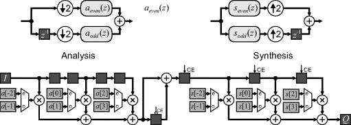
For the analysis filter, this still means that all of the multiplications are performed in a single clock cycle, but only need to be evaluated every second cycle. The hardware may be reduced by calculating the even and odd filters in alternate clock cycles. The result of the even filter is held for one cycle and added to that from the odd filter.
For the synthesis filter, the incoming data is only clocked every second cycle. On the output, the results are produced alternately by the even and odd filters. This enables a single filter to be used, by just multiplexing the coefficients.
For a given wavelet, the filter coefficients are constant. Therefore, the multiplexers selecting the filter coefficients can be optimised away, resulting in a very efficient implementation. Only a single side of the wavelet filtering is shown in Figure 10.22; two such circuits are required, one of the low pass filter and one for the high pass filter.
10.3.1.3 Lifting Scheme
The filtering can be optimised further. The designs so far assume that the low and high pass filters are independent. However, these filters are closely related because they are pair-wise complementary. The polyphase filters for both the low and high pass filtering may be written in matrix form:
(10.55) ![]()
The relationship between the filters allows this filter matrix to be factorised (Daubechies and Sweldens, 1998):
(10.56) ![]()
where each of the ![]() is usually a constant or first order filter. Each of the terms on the right is a lifting step, resulting in the implementation of Figure 10.23. In general, this will reduce the number of multiplications by a further factor of two.
is usually a constant or first order filter. Each of the terms on the right is a lifting step, resulting in the implementation of Figure 10.23. In general, this will reduce the number of multiplications by a further factor of two.
Figure 10.23 Lifting implementation of wavelet filters.

A second advantage of using lifting steps is that even with quantisation of the filter coefficients and rounding of the outputs of the ![]() filters, the output is perfectly recoverable. This is because the synthesis filter just undoes the steps of the analysis filter, subtracting off the terms that were added in. Any quantisation within the synthesis filter will be exactly the same as that in the analysis filter, recreating the data back along the filter chain.
filters, the output is perfectly recoverable. This is because the synthesis filter just undoes the steps of the analysis filter, subtracting off the terms that were added in. Any quantisation within the synthesis filter will be exactly the same as that in the analysis filter, recreating the data back along the filter chain.
In this context, the scaling terms (by ![]() and
and ![]() ) can also be implemented using lifting steps as well, to enable rounding errors from the scaling to also be recovered exactly (Daubechies and Sweldens, 1998):
) can also be implemented using lifting steps as well, to enable rounding errors from the scaling to also be recovered exactly (Daubechies and Sweldens, 1998):
(10.57) 
This requires three extra lifting steps, since the first step is in parallel with the last filtering step, so can be combined with it. If wavelet coding is being used for lossy image compression, the ![]() and
and ![]() outputs will be quantised. In this case, the scaling terms can be incorporated into the quantisation stage without any additional operations.
outputs will be quantised. In this case, the scaling terms can be incorporated into the quantisation stage without any additional operations.
One limitation of using lifting for implementing the wavelet transform is that all of the operations are now in series, rather than in parallel as with the direct and polyphase implementations. Consequently, the latency is increased relative to the direct or polyphase implementations, although the filters can readily be pipelined to maintain the required throughput.
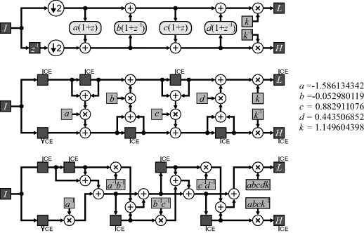
An implementation of the 9/7 biorthogonal wavelet analysis filter is shown in the centre panel of Figure 10.24, which shows five multiplications and eight additions in series on the critical path. (Note that all of the registers are clocked only every second cycle.) Huang et al. (2004) address the problem of increased latency by identifying the critical path, and replace multiplications (which tend to be the most time consuming operation) on the critical path with a multiplication by the inverse on the corresponding parallel path. One implementation which removes all but two of the multiplications and half of the additions from the critical path is shown in the bottom of Figure 10.24. Note that this implementation loses the prefect reconstruction property of the standard lifting scheme.
Figure 10.24 Implementation of the 9/7 biorthogonal analysis wavelet filter. Top: basic lifting schematic; centre: hardware implementation; bottom: removing multipliers from the critical path.
Rather than rearrange the circuit, the latency can be accepted, with pipelining used to maintain the throughput. All of the filtering is performed after down-sampling, so the filters only process one sample every second clock cycle. Since each stage of the filter has the same architecture, this allows the filter to be half the length, with the second half using the second clock cycle. Alternatively, the full filter could be implemented with two rows (or columns) transformed in parallel if the input bandwidth allows. Another possibility is to feed the low pass output back to the input and use the spare cycles for subsequent levels within the decomposition (Liao et al., 2004).
10.3.1.4 Two-Dimensional Implementations
The descriptions above were for one-dimensional filters. When extending to two dimensions, three approaches are commonly used. The simplest approach is to alternate the row and column processing. This requires processing all of the rows first, saving the intermediate results in off-chip RAM. The columns are then processed, returning the results to off-chip memory. This procedure is then repeated for the LL band for each level of decomposition. Since each row and column is processed independently, the direct separable approach is easy to accelerate through multiple parallel processors, subject of course to memory bandwidth limitations.
A second approach is to begin the column processing as the processed row data becomes available. This requires replacing delays within the filter with on-chip row buffers, enabling all of the columns to be processed in parallel (Chrysafis and Ortega, 2000). This fits the stream processing model and completely transforms the image as it is being streamed into the FPGA. If the wavelet transform is the end of the processing, the wavelet coefficients can be streamed to off-chip memory as they are calculated. However, if further processing is required, additional caching is required to hold the results from the lower decomposition levels while the transformation is being performed on the higher levels. The amount of synchronisation memory grows rapidly with the number of decomposition levels (Chrysafis and Ortega, 2000). The line processing approach is also a little harder to parallelise. Like the separable approach, multiple rows may be processed in parallel. Processing rows in pairs will also provide the data for column processing two samples at a time. This makes full use of the available clock cycles on the down-sampled data. Alternatively, the spare cycles may be used for processing subsequent decomposition levels (Liao et al., 2004). One aspect to consider is that, rather than multiplexing individual registers, using dual-port fabric RAM builds in the multiplexers for free and may reduce the resources required.
The on-chip memory requirements of the line processing approach may be reduced by dividing the image into blocks and transforming the image a block at a time. The input blocks need to overlap because data from adjacent blocks is required to correctly calculate the pixels around the block boundaries. The block processing approach is also readily parallelisable, although coordination is required when accessing those pixels which are shared between blocks. However, if the resources allow, it is simpler to use line processing rather than process multiple blocks in parallel.
Angelopoulou et al.,) compared these three methods for FPGA implementation. The direct separable approach used the fewest resources because it was the simplest architecture, but also took the longest because the data must be accessed multiple times. The best in terms of total time and power was the line buffered approach. Block-based processing has smallest memory requirement, but has the most complex logic because of the need to manage the block boundaries.
10.3.2 Applications of the Wavelet Transform
As with the Fourier transform, wavelets have a wide range of applications within image processing. While a full discussion is beyond the scope of this book, some of the main applications are introduced in this Section.
One of the most significant applications of the wavelet transform is in image compression. The steps involved in compressing images are described more fully in Section 10.4. The wavelet transform is used primarily to decorrelate the data. Adjacent pixels in many images are similar and this is exploited by separating the approximation and detail components. As demonstrated in Figure 10.20, the image is sparse within the wavelet domain, with many detail coefficients zero or close to zero. Truncating these coefficients provides an effective means of lossy compression that has a low impact on the perceived image quality.
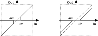
If an image has noise added, this noise will be most noticeable in the detail coefficients. Noise will affect all of the coefficients, but since the wavelet representation is generally sparse, setting the coefficients below a threshold to zero will remove the noise from those terms. When the image is reconstructed with an inverse wavelet transform, the noise will be reduced. This is called hard thresholding and has the characteristic that it preserves features such as peak heights (Donoho and Johnstone, 1994). An alternative approach is soft thresholding, where all of the wavelet coefficients are shrunk towards zero (the two approaches are compared in Figure 10.25). Soft thresholding tends to give a smoother fit and does not result in the same level of lumpiness that normally results from smoothing noise (Donoho, 1995). The threshold for both methods is proportional to the noise standard deviation in the image. These simple approaches assume that all coefficients are independent. However, there is a strong correlation between detail coefficients at different levels of decomposition. More sophisticated denoising techniques take into consideration these correlations (Sendur and Selesnick, 2002), giving better noise reduction.
Figure 10.25 Thresholding of wavelet coefficients for denoising. Left: hard thresholding; right: soft thresholding.
Multiscale processing has been mentioned in several contexts throughout this book. Wavelets provide a natural framework for multiscale object detection (Strickland and Hahn, 1997), although relatively little work has been reported on FPGA implementations.
A final application considered here is the fusion of images from different sources. It will be assumed that the images have already been registered; this topic has been covered in some detail in the previous chapter. Image fusion is therefore concerned primarily with combining the data from each of the images in a way that provides a higher quality (in some sense of the word) output image. This can range from simple averaging to reduce noise, through to combining data from disparate imaging modalities (for example positron emission tomography and magnetic resonance images, or multiple spectral bands) and image super-resolution, where the output data has higher resolution than the input. In the context of wavelet processing, each of the registered input images is decomposed through the wavelet transform, the wavelet coefficients are then merged in some way and the result inverse wavelet transformed (Pajares and de la Cruz, 2004).
If the coefficients are simply averaged, then the wavelet transform (being linear) is not necessary unless the images are of different resolution. One method of merging the wavelet coefficients that is surprisingly effective is to simply select the coefficient with the maximum absolute value from the input images. This can readily be extended to filtering within the wavelet domain before selecting, or using consistency verification to ensure that groups of adjacent coefficients are consistently selected from the same image (Pajares and de la Cruz, 2004). A classic example of image fusion is focus extension in microscopy of extended objects. With a thick object, the complete object cannot be brought into focus simultaneously – as the focus is adjusted, different parts of the object come into and out of focus. The in-focus components of each image will have higher local contrast, resulting in a larger magnitude within the detail coefficients. Selecting the components with the maximum absolute values will select the parts of the image that are most in focus within the set, with the fused output image having an extended focus range (Forster et al., 2004).
The information content within images and video may be compressed to reduce the volume of data for storage, or to reduce the bandwidth required to transmit data from one point to another (for example over a network). Images are able to be compressed because they contain significant redundancy.
There are at least four types of redundancy within images. Spatial redundancy results from the high correlation between adjacent pixels. Since adjacent pixels are likely to come from the same object, knowing the value of one pixel can enable the value of adjacent pixels to be predicted. Similarly, there is temporal redundancy between the frames in a video sequence. Successive frames are likely to be very similar, especially if there is limited movement within the sequence. If any movement can be estimated, then the correlation can be increased further through motion compensation. Spectral redundancy reflects the correlation between the colour components of a standard RGB image, especially when looking at natural scenes. Finally, psycho-visual redundancy results from the fact that the human visual system has limited resolution, both spatially and in terms of intensity, and is tolerant of errors or noise within textured regions.
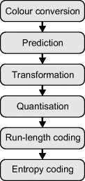
All of these factors enable image data to be compressed by reducing the redundancy. The six basic steps commonly used in compressing an image or video sequence are listed in Figure 10.26. These are outlined briefly in the following paragraphs.
Figure 10.26 Steps within image or video compression.
10.4.1.1 Colour Conversion
Colour images are usually converted from RGB to YCbCr for two reasons. Firstly, most of the variation within images is in intensity. Therefore, the conversion will concentrate most of the signal energy into the luminance component. The weights used for the RGB to YCbCr conversion (Section 6.3) correspond to the relative sensitivities of the human visual system, and this transformation is used with many codecs. Alternatively, the reversible colour transform of Equation 6.57 can also be used by JPEG 2000 (ISO, 2000).
The lower colour spatial resolution of the human visual system enables the chrominance components to down-sampled by a factor of two without any significant loss of subjective quality. This down-sampling is optional and is automatically handled with wavelet-based compression by the first wavelet scale.
10.4.1.2 Prediction
Prediction uses the pixels already available to predict the value of the next pixel (or block of pixels). The residual, or prediction error, has a tighter distribution enabling it to be coded with fewer bits. It is most commonly used with lossless coding methods, where prediction can typically give 2:1 compression. However, it is less often used directly with lossy image coding. Lossy JPEG coding only uses prediction of the DC component between horizontally adjacent blocks. Prediction is used in intra-frame coding within H.264 with a number of different prediction modes.
One of the most common uses of prediction is in inter-frame coding of video. A video sequence is usually divided into groups of pictures (Figure 10.27). The first frame within the group is coded independently of the other frames using intra-frame coding, and is denoted an I-frame. Then, motion compensated forward prediction is used to predict each P-frame from the previous I- or P-frame. Finally, bi-directional (both forward and backward) prediction is then used to predict the intervening frames, denoted B-frames. The B-frames usually require the least data because the backward prediction is effective at predicting the background when objects have moved away. The number of P- and B-frames in each group of pictures depends on the particular codec and application.
Figure 10.27 Prediction within a group of pictures, showing the relationships between I, P and B frames.

Motion compensated prediction divides the image into 8 × 8 or 16 × 16 blocks and usually uses the sum of absolute differences to find the offset that minimises the prediction error (as described in Section 9.5.2). This is an effective method of reducing the redundancy when the motion is within the search window. Since the B-frames require the following P-frame (or I-frame), the frames are not transmitted in their natural order, but the order in which they are required to decode the sequence. This means that the encoder must be able to hold several uncompressed B-frames until the following P-frame (or I-frame) is available. The decoder is a little simpler, in that it always only needs to hold the two frames used for providing motion compensated source data.
To be most effective, it is necessary for the encoder to decode the frame before using it to make a prediction so that the data will match that available at the receiver. Otherwise, any quantisation errors in the prediction will not be taken into account and can propagate from one P-frame to the next. This decoding requires an inverse transform to convert the quantised coefficients back to pixel values. Unfortunately, the encoder has little control over the implementation of the inverse transform in the receiver. With a single image codec, this does not matter, but with video the differences in round-off error can accumulate from frame to frame, causing the prediction made at the receiver to drift. This requires care with the design of the inverse transform used at both the encoder and receiver (Reznik et al., 2007).
10.4.1.3 Transformation
The primary purpose of image transformation within an image coding context is to concentrate the energy into as few components as possible. This exploits the spatial correlation within images. Different compression methods use different transformations. Two of the most commonly used transforms are the discrete cosine transform, used with JPEG, MPEG, and the wavelet transform, used with JPEG 2000.
The discrete cosine transform is close to the optimal linear transform for decorrelating the pixel values. This makes it an obvious choice for image compression. However, with global transforms every coefficient depends on every input pixel. Therefore, the image is usually divided into smaller blocks, which are transformed independently. JPEG performs a discrete cosine transform on 8 × 8 blocks. One limitation of dividing the image into blocks is that, since each block is encoded independently, there is a loss of coherence at block boundaries. After quantisation, this can lead to blocking artefacts – the appearance of false edges at block boundaries, especially at high compression rates. These can be reduced to some extent by filtering the image after decoding (Vinh and Kim, 2010).
The wavelet transform operates locally rather than globally, reducing the need to split the image into blocks. JPEG 2000 allows large images to be split into large blocks or tiles to reduce the memory requirements when coding or decoding. Wavelets compact most of the energy into the low frequency coefficients, giving good energy compaction. The high frequency components are concentrated on edges, with a significant number of small or zero coefficients, enabling effective compression.
Another advantage of using the wavelet transform is that it is easy to reconstruct an output image at a range of different scales simply by choosing which level of wavelet coefficients are used in the reconstruction.
10.4.1.4 Quantisation
Transformation just rearranges the data, which is completely recoverable via the corresponding inverse transformation (in practise, if the coefficients are not integers, then rounding errors can make the transformation irreversible). The next step in the coding process, quantisation, is lossy in that the reconstructed image will only be an approximation to the original. However, it is the quantisation of the coefficients that can enable the volume of data used to represent the image to be compressed significantly. With coarser quantisation steps, fewer values are used and the greater the compression. However, more information will be lost and this can reduce the quality of the reconstructed image or video.
Quantisation divides the range of input values into a number of discrete bins by specifying a set of increasing threshold levels. It is this many-to-one mapping that makes quantisation irreversible. When reconstructing the value, the centre value for the bin is usually used. The difference between the original value and the reconstructed output is the error or noise introduced by the quantisation process. Since it is usually the transform coefficients that are quantised rather than the input pixel values, the errors do not normally appear as random noise within the image. Typically, quantisation errors show in the image as blurring of fine detail and ringing around sharp edges.
The optimal quantiser adjusts the quantisation thresholds to minimise the mean square error for a given number of quantisation levels. This makes the bins smaller where there are many similar values, reducing the error, at the expense of increasing the error where there are fewer values. This tends to make the bin occupancy more uniform, reducing the gains of entropy coding. The optimal quantiser is data dependent, so requires the levels to be transmitted with the compressed data, reducing compression efficiency. A similar effect may be achieved without the overhead by using a predefined nonlinear mapping followed by uniform quantisation (where the threshold levels are equally spaced). For image compression, however, the gains from using optimal quantisation are not sufficiently significant to warrant the additional complexity; it is easier to simply use uniform quantisation with a finer step size and rely on entropy coding to exploit the fact that some bins are relatively empty.
For image compression, different transformed coefficients have different visual significance, so different quantisation step sizes are used for each coefficient. JPEG has tables specifying the quantisation step sizes for each coefficient; ‘standard’ tables are given in Figure 10.28 (ISO, 1992; Wallace, 1992). If the DCT coefficients are ![]() and the quantisation table is
and the quantisation table is ![]() , then the quantised coefficients are:
, then the quantised coefficients are:
(10.58) ![]()
Figure 10.28 JPEG compression (ISO, 1992). Left: standard luminance and chrominance quantisation tables; right: zigzag coding order.

Any scale factors associated with the DCT can be directly included into the quantisation step. This requires two tables to be used: one for actually performing the quantisation and the other which is saved with the data as part of the JPEG output file.
A single quality factor parameter can be used to scale the quantisation step size to control the compression (and consequently the image quality). The implementation within the open source IJG JPEG codec uses a quality factor, ![]() , that varies from 1 to 100 to scale the standard quantisation tables as follows:
, that varies from 1 to 100 to scale the standard quantisation tables as follows:
(10.59) 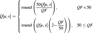
with any values that go to zero set to 1.
JPEG2000 uses a bit-plane coding approach to control quality. In the output data stream, the data is encoded in bit-plane order with the most significant bit encoded first, through to the least significant bit last. The EBCOT algorithm (Taubman, 2000) divides the tree into blocks and performs coding in multiple passes at each wavelet layer to ensure that the bits are in order of their significance in terms of contributing to the quality of the final image. This enables the coding for each block to be truncated optimally to minimise the distortion while controlling the bit-rate of the final output stream. One FPGA implementation of EBCOT algorithm has been described by Gangadhar and Bhatia (2003).
10.4.1.5 Run-Length Coding
Line drawings, and other related graphics, have a limited number of pixel values, and these often occur in long runs. This makes run-length encoding of such images an effective compression technique.
Many transform techniques have a large proportion of the coefficients close to zero. Having a dead band – a wider bin for zero – gives more zero coefficients and enables run-length coding to be used to compress successive runs of zeros. This is used in two ways: one is true run-length coding, where a symbol and count are output; the other is to have a special zero-to-end symbol, which indicates that all of the remaining symbols to the end of the block are zero. This latter approach is effective both with the block-based coding used by JPEG and also with wavelet coding, eliminating whole trees of zero coefficients, especially for the more significant bits when bit-plane coding is used.
With block-based coding, many of the high frequency components are zero. These can be placed at the end of the block by storing the coefficients in the zigzag order shown in Figure 10.28. This enables many coefficients to be compressed by a single zero-to-end symbol. Zigzag reordering may be implemented efficiently by having a lookup table on the address lines, as shown in Figure 10.29. If the coefficients are not in their natural order, for example if the DCT produces a permuted output, then the zigzag lookup table can also take this into account. A similar lookup table based addressing technique can be used when decoding the images.
Figure 10.29 Implementation of zigzag reordering.
10.4.1.6 Entropy Coding
The final stage within the coding process is entropy coding. This assigns a variable length code to each symbol in the output stream based on frequency of occurrence. Symbols which appear frequently are given short codes, while the less common symbols are given longer codes. The entropy of a stream is:
(10.60) ![]()
where ![]() is the probability of the
is the probability of the ![]() th symbol. The entropy gives a lower bound on the average number of bits used to represent the symbols. For N different symbols, the entropy will be between zero and
th symbol. The entropy gives a lower bound on the average number of bits used to represent the symbols. For N different symbols, the entropy will be between zero and ![]() , with the maximum occurring when all symbols are equally probable.
, with the maximum occurring when all symbols are equally probable.
One of the most common forms of entropy coding is Huffman coding (Huffman, 1952). This uses the optimum number of bits for each symbol. The Huffman code is built by sorting the symbols in order of probability and building a tree by successively combining the two symbols with the least probability. The length of each branch is the number of bits needed for the corresponding symbol. The main limitation of Huffman coding is that an integer number of bits is required for each symbol. Consequently, the average symbol length will be greater than the entropy. In particular, symbols with probability greater than 50% will always require one bit, even though the entropy is lower. This may be improved by grouping multiple symbols together and encoding symbol groups. A second limitation is that an overhead is incurred in representing the coding table (the mapping between a symbol and its code) since this is data dependent. Although there is no default Huffman table in JPEG, a typical table is provided with the standard based on a large number of images. Using this table saves having to gather the statistics from the image before coding. There are techniques for efficient compression of the coding table (Body and Bailey, 1998), although these are not currently used by any standard.
JPEG combines the run length with the size of the coefficient to form an 8-bit symbol which is Huffman coded, followed by the actual coefficient. A block diagram of a possible Huffman coding module for JPEG compression is shown in Figure 10.30. The run length of zeros is provided with each non-zero coefficient as input. The encoding block determines the length of the value, ![]() , and encodes it in the available bits,
, and encodes it in the available bits, ![]() . The value length is combined with the zero run length, giving an 8-bit symbol for Huffman coding. The coded symbol is restricted to 16 bits length, so a lookup table based approach therefore requires a 256 × (16 + 4) lookup table to provide the
. The value length is combined with the zero run length, giving an 8-bit symbol for Huffman coding. The coded symbol is restricted to 16 bits length, so a lookup table based approach therefore requires a 256 × (16 + 4) lookup table to provide the ![]() and associated length,
and associated length, ![]() . The
. The ![]() and
and ![]() are concatenated and barrel shifted to align with the
are concatenated and barrel shifted to align with the ![]() bits. The lengths are added to the
bits. The lengths are added to the ![]() with the carry used to determine how many bytes are shifted out.
with the carry used to determine how many bytes are shifted out.
Figure 10.30 Huffman coding for JPEG.
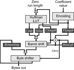
Using a custom table with JPEG requires performing the initial coding steps without the final Huffman coding. The symbols and quantised coefficients need to be saved in a frame buffer while a histogram is used to gather the statistics on the particular symbols used. The histogram then needs to be sorted and the Huffman tree built. The final step is then to Huffman encode the data from the frame buffer.
A table approach can also be used for Huffman decoding. Brute force decoding would require 216 entries to perform the decoding. However, by segmenting the address space (decoding fewer bits at a time), smaller tables can be used, although at the expense of more clock cycles (Body and Bailey, 1998). This is practical because run-length coding of the zeros means that a value need not be decoded every clock cycle. An alternative approach has been described by Sun and Lee (2003) based on counting the number of leading ones and using this to select the table for decoding. This works because the longer code words tend to begin with a relatively long sequence of ones.
Arithmetic coding removes the restriction of having an integer number of bits per symbol. It encodes the whole stream as an extended binary number, representing a proportion between 0 and 1 (Rissanen, 1976; Langdon, 1984; Witten et al., 1987). Each symbol successively divides the remaining space in proportion to its probability. The key to an efficient implementation is to work with finite precision and output the leading bits once they can no longer be affected. Using finite precision (and rounding) introduces a small overhead over the theoretical minimum length. There is also an overhead associated with specifying the symbol probabilities.
The basic structure of an arithmetic coder is shown in Figure 10.31. The ![]() and
and ![]() registers hold the start and width of the current range. At the start of coding they are initialised to 0 and 1 respectively. The symbol to be coded is looked up in a table to determine the start and width of the symbol. These are scaled by the current
registers hold the start and width of the current range. At the start of coding they are initialised to 0 and 1 respectively. The symbol to be coded is looked up in a table to determine the start and width of the symbol. These are scaled by the current ![]() to give the new
to give the new ![]() and
and ![]() remaining. The renormalisation block renormalises the variables and outputs completed bits. The carry propagation records the number of successive
remaining. The renormalisation block renormalises the variables and outputs completed bits. The carry propagation records the number of successive ![]() output, because a carry can cause these to switch to zeros (Witten et al., 1987).
output, because a carry can cause these to switch to zeros (Witten et al., 1987).
Figure 10.31 Basic structure of arithmetic coding.
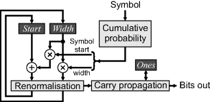
The overhead associated with initially specifying the initial probabilities may be overcome by adaptive coding. This builds the table of probabilities as the data arrives. While adaptive coding can be used with either Huffman or arithmetic coding, it is less convenient with Huffman coding because changing the symbol probabilities requires completely rebuilding the code tree. Since arithmetic coding works directly with the probabilities, this is less of a problem. There are two approaches to adaptive coding. The first is to assume each symbol is equally likely (with a count of one), with the count incremented and probabilities adjusted as the symbols arrive. There is an overhead resulting from overweighting rare symbols at the start. The second approach is to have an empty table, except for an escape symbol, which is used to introduce each new symbol.
Adaptive coding is good for very short sequences where the overhead of the table can be larger than the actual sequence itself, especially if there is a large number of symbols compared to the length of sequence. It also works well for long sequences because the statistics approach the optimum for the data, although there is an overhead at the start while the table is adapting to the true probabilities. If the statistics are not stationary, then periodic rescaling of the counts (for example dividing them all by a power of two) enables the probabilities to track that of the more recent data.
One final class of compression methods that will be mentioned briefly is that of dynamic dictionary based methods. These allow sequences of symbols to be combined and represented as a single symbol. The original method in this class is LZ77 (Ziv and Lempel, 1977), which uses as its dictionary a window into the past samples. A sequence of symbols that has already been encountered is coded as an offset plus length. LZ77 is combined with Huffman coding to give the DEFLATE algorithm (Deutsch, 1996), used to encode PNG image files. The search through past entries can be accelerated through the use of a hash table to locate potential candidate strings. Alternatively, a systolic array may be used to perform the search (Abd Elghany et al., 2007). A related variation is the LZW algorithm (Welch, 1984), which explicitly builds a dictionary on-the-fly by extending existing sequences each time a new combination is encountered. LZW is used to compress GIF image files.

