
Chapter 15
Ground-based Deformable Antennas1
15.1. Introduction
RADAR systems are designed to localize and characterize non-cooperative moving targets. They allow a precise angular localization thanks to the high directivity of their antennas. Directivity is a function of the size of the antenna and of the radio frequency wavelength. It is given by the radiation pattern, a mathematical function providing the evolution of the electromagnetic waves emitted or received by an antenna according to the spatial coordinates. To guarantee optimal performances, these antennas must be perfectly flat. Constraints in positioning antenna sub-arrays along a reference surface with an accuracy below a few millimeters or along a reference angle of few milliradian lead either to a significant weight of the sandwich-type structures or to an important volume and weight of the supporting structure.
Surface radar systems on ground and naval carriers require an improvement of structural and RF performance flexibility to provide low cost solutions with better tactical deployment and to open new capacities of implementation on non-dedicated platforms.
Recent developments in radar front-end technology show a clear trend towards miniaturization of electronic components for transmitting and receiving chains. Integration of the electronics will enable us to achieve very thin antenna arrays. As a result, the supporting structure of the antenna becomes subject to mechanical distortions entailed by the operating environment among which unsteady aerodynamic loads such as wind, turbulence or explosion blast, thermal distortions due to the assembly of different materials, static loads including water, ice and snow loads, mechanical vibrations arising from rotation, especially on ground based platforms, or pitch, roll and engines, effects on ships.
Distortions on large active antenna structures cause significant degradations of their radiation pattern, and consequently of radar performances. As the use of complete electronically steered arrays allows an accurate control of RF waves, we propose here to dynamically cope with distortions of radars in S-band (fRF=3 GHz) with an innovative two-step method. In a first step, the antenna shape is captured via an optical sensor; afterwards the global radiation pattern is reshaped using a computed phase law applied on the RF signals.
The first section is dedicated to the quantification of the impact of distortions on radar systems (pointing error and effect on radial velocity measurement). Secondly, we focus on the antenna shape sensor. Due to the harsh environment, the measurement must be distributed along the surface. Two sensor principles are eligible. They are both based on the interception of a laser plane acting as an absolute flat reference. The first is based on the use of an imaging fiber device, the second on a measurement of light polarization. Electromagnetic immunity is guaranteed by the use of optical fibers to transmit laser light behind the radiating surface. With the knowledge of radiating elements positioning along the surface, a compensation feedback law is proposed to mitigate distortions effect. High quality radiation patterns are recovered and radar system performances are preserved. The simplicity and lightness of computation are mandatory to allow true time compensation on large 2D arrays witnessing distortions. Finally, we illustrate this concept with a large deformable antenna mock-up.
15.2. Impact of antenna distortions on radar systems
15.2.1. Array factor of deformed antennas
It is essential to know the behavior of an antenna subject to deformations. Even though mechanical amplitudes are weak, they may be significant considering radiation requirements on such systems.
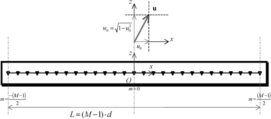
An array antenna is the association of elementary antennas fed by a distribution network [JAS 61]. We consider M × N elements periodically distributed with regular spacing dx and dy respectively along the Ox and Oy axis (Figures 15.1 and 15.2).
We will characterize specific impacts induced on the radiation pattern for different types of standard deformations. Calculations are made considering the difference between deformed position and nominal position of radiating elements (Figure 15.2). Translations and rotations of the whole radiating surface are not considered here because radiating elements used have broad radiation patterns and the displacements considered only modify their orientation by a few degrees.
Figure 15.1. Coordinate system
Figure 15.2. Representation of a regular antenna array (xOy): (left) general pattern; (right) displacement of an element
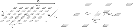
The phase shift between electromagnetic fields emitted by each radiating element is directly proportional to the displacement along the three axes relative to the nominal position in the network. The position of an element S (m, n) on the deformed array is described with respect to the reference source by the following vector:
[15.1] ![]()
The array factor describing the radiation pattern of a deformed antenna is then:
[15.2] ![]()
with fm, n the complex excitation coefficient of the (m, n) element and k the wave number (k=2.π/λ). It is important to notice that mechanical errors are not frequency dependant and non-stationary with the observation angle.
Figure 15.3 shows a deformation of a linear 27 element antenna in S band, representative of even deformations caused by wind or by the first natural vibration mode of the antenna structure. The “sum” radiation pattern of the deformed array calculated with equation [15.2] (all elements are in phase) is compared with the “sum” pattern of the non-deformed antenna for a pointing direction θp=−20°.
Figure 15.3. a) First distortion of the linear antenna; b) radiation pattern of the linear antenna witnessing the first distortion
We can notice three important points:
– The main beam is always pointing in the correct direction θp.
– The main beam is significantly broadened, and consequently the gain is decreased compared to the ideal antenna.
– The average transverse displacement of radiating elements is not zero. In other words, we notice a translation of the mean position of the antenna. The phase center of the antenna is shifted resulting in a phase variation of received signals.
Figure 15.4 shows a deformation of a linear 27 element antenna in S-band, representative of odd deformations caused by an angular acceleration due to rotation around the central axis or by the second natural vibration mode of the antenna structure.
Figure 15.4. a) Second distortion of the linear antenna; b) radiation pattern of the linear antenna witnessing the second distortion
Similarly, three important points are to be observed:
– The antenna is no longer pointing in the direction θp. Pointing direction is strongly affected by such deformations. The displacement of radiating elements acts as a phase ramp. The main beam is steered by several degrees.
– Antenna gain in the pointing direction is strongly attenuated, while the maximum gain of the antenna is virtually unchanged. However, we notice a high side lobe whose amplitude is located −15 dB below the amplitude of the main lobe, instead of the −40 dB desired.
– The average transverse displacement of radiating elements is low. Phase shift of received signals in the pointed direction is moderate.
15.2.2. Impact on antenna pointing
Starting from the classical pointing criterion, we will calculate the error made with respect to a deformation. From equation [15.2], and assuming small variations in position compared to the wavelength, instead of being cancelled in the direction u0 (corresponding to the angle θp) the pointing criterion will be cancelled in u0 + δu0. Let b be a “difference” excitation law (odd with variable m and even with the variable n) and be the δu0 pointing error along the axis (Ox). A simple calculation gives the pointing error for a 2D antenna along the axis (Ox):
![]()
with:
[15.3] 
Thus, even deformations will not change the pointing direction. On the contrary, odd deformations will strongly steer the beam.
The effective pointing direction is calculated assuming small deformations by performing the scalar product of directivity vectors u0 and u0 + δu0. Calculation directly gives access to cos(δθ), with the angle difference δθ between the two vectors. We can obtain an expression with two independent variables δu and δv:
[15.4] ![]()
If we consider the case of the 27 element linear array, the pointing error is δθ = 2.25°, almost 40 milliradian for the odd deformation shown in Figure 15.4. This error caused by an amplitude variation of about λ/2 = 5 cm is not acceptable for most applications. For ground-based radars, the desired accuracy is about a few milliradians.
The precision of the angular localization of a target totally depends on the ability of the antenna to observe a direction of space. The result is a bias in the estimation of the target angular location.
15.2.3. Parameters of targets in the pointing direction
In addition to the tracking error mentioned above, the phase variations will affect the detection and estimation of target parameters. The accuracy in distance, and especially in radial velocity, mainly depends on the stability at the scale of the pulse burst. Phase shift of transmitted and received signals, caused by the motion of the antenna, will bias the estimation of the Doppler frequency.
Ground-based antenna structures have low natural vibration frequencies, comparable to the radar pulse repetition frequency (< 100 Hz). It is often wise not to consider variation of amplitude and phase into the pulse, given the ratio of 100 between the pulse duration (~ 100 μs) and minimal vibration period of considered distortions (~ 10 ms).
Distance estimation is based on the measurement of the pulse time of flight [CHE 89]. This measurement will be affected only if the deformation amplitude is comparable to the distance between the radar and the target. We can reasonably assume that this is not the case. The estimated distance is not affected by the deformations of the antenna.
The estimation of target velocity is strongly affected by the phase shift of the received signals. The phase shift from pulse to pulse will entail the Doppler frequency measurement and therefore the measurement of target radial velocity.
The successive phase measurements give access to the Doppler frequency [CHE 89]. A phase shift due to deformation is interpreted as a shift in the Doppler frequency. Figure 15.5 shows an example of Doppler spectrum degradation caused by an even shape at 10 Hz.
Figure 15.5. a) Phase shift caused by the deformation; b) Doppler spectrum for a 10 Hz deformation – 49 pulses, duration 100 μs, and repetition period 1 ms
In this case, we notice a 24 Hz translation of the spectrum, i.e. 8% relative error on the real radial velocity of the target. The error is not negligible, since this translation is not very different from the spacing between two Doppler filters. The translation also affects the clutter rejection. Without a change of the rejection band, we may detect low speed false targets.
For faster deformation, we have a phase modulation causing new lobes in the frequency spectrum. Figure 15.6 shows the Doppler spectrum for a 60 Hz deformation with a π/4 amplitude phase shift.
Figure 15.6. a) Phase shift caused by the deformation; b) Doppler spectrum for a 60 Hz deformation – 49 pulses, duration 100 μs, and repetition period 1 ms
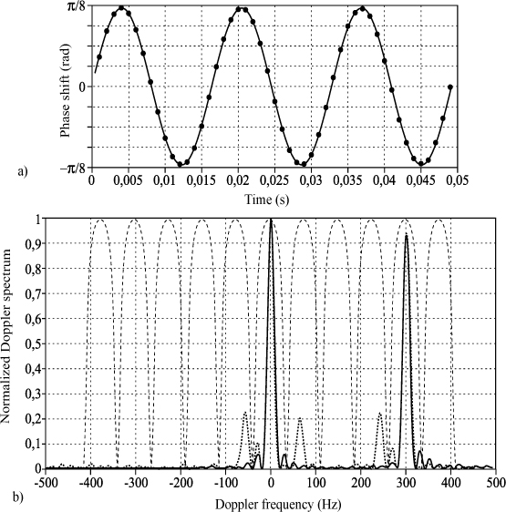
Phase shift creates high modulation lobes and increases the residual power in adjacent filters. If the amplitude of the phase shift is too large, the radar will detect false targets. The amplitude of the false target signals depends on the signal strength and the maximum amplitude of the phase shift introduced by the antenna. Note that in most cases, the signal from the target is very small compared to the clutter. False targets around the target will probably not be detectable. The risk for radar application is mostly the detection of a false target at low speed due to the modulation of the clutter phase.
15.2.4. Conclusion and compensation method
Mechanical errors are frequency-independent and non-stationary with the observation direction. They cannot be eliminated by calibration because they dynamically change with external conditions.
In the radar application context, deformation disturbances are often unacceptable:
– The pointing accuracy requirement is about a few milliradians, but variations of the radiation pattern causes an error of several degrees on the angular location of targets.
– The estimation of the radial velocity is based on the stability at the timescale of the burst. Dynamic shape variations add substantial and variable bias in the measured Doppler frequency.
To be efficient, the compensation applied to the antenna must correct the pointing direction of the antenna close to a few milliradians. Then, it must retain as low a level of side lobes as possible (in reference to the ideal antenna) to avoid adding noise to the signal.
The instrumented method proposed is based on two points:
– The real time sensor developed is distributed along the antenna, and is eligible for a rotating radiating surface.
– The compensation algorithm takes into account the whole radiation pattern of the antenna. The developed method is to recover the radiation pattern in all directions simultaneously.
15.3. Instrumentation of deformable antennas
15.3.1. Mechanical analysis
In current systems, mechanical structures are massive in order to maintain the flatness of the radiating surface below several percent of the wavelength. Preliminary experiments shown that the environment of the antenna can be modeled with a limited number of loading cases depending on the application, basement and environment of the radar. Consequently, all deformations witnessed by an antenna are measurable with a limited number of sensors.
Deformation causes can then be identified as follows:
– additional quasi-static loads (antenna dead load, snow or ice) and dynamic loads (wind, blast, rain and hail);
– mechanical vibrations and random impulses (engines and gear noise arising from the rotation of the antenna);
– thermal deformations (assembly of materials having different thermal expansion coefficients).
15.3.2. Optical Sensor
The optical sensor developed must be able to measure the transverse displacement of a flexible antenna. The maximum amplitude of the deformations today are about 1 mm over the whole radiating surface, so the plan is to design an optical sensor with 40 mm dynamics, industrial processes impose this limitation.
Two main characteristics are taken into account in the implementation of these sensors. The first is to have sufficient precision on the transverse displacement in order to implement the compensation and recover the performance of a nondeformed antenna. The second is related to the highly electromagnetically perturbed environment of the antenna.
The environment of an antenna is a major constraint on the development of the sensor. RF pulses average power ranges from 1 W to 100 kW, with peak power up to 1 MW. Sensors require a high galvanic isolation of the complete measuring chain embedded on the surface of the antenna. Here are the specifications of the sensors:
– dynamic range 40 mm, resolution <100 microns, bandwidth 250 Hz;
– electromagnetic compatibility (immunity to the intense electromagnetic fields radiated by the antenna and no change of radiation pattern of the antenna linked to the presence of the sensor);
– suitable for real-time processing;
– ease of integration to a rotating array antenna structure and ability to be adapted to different antenna configurations;
– measurement time interval short enough to make an efficient compensation;
– lifetime equivalent to the radar system (~ 20 years);
– low cost (a few k € for the whole measurement system).
The principle is to generate a reference laser plane parallel to the antenna surface. It is intercepted by a set of N passive optical probes, placed at specific locations where the information of local deformation will enable the global reconstruction of the antenna shape. The probes are designed to transmit the local variations of transverse deformation relative to the reference plane via optical fibers, to photo-detectors under the surface of the antenna. In this way, electronics for sensing and signal processing are isolated from electromagnetic radiations emitted by the antenna.
Two solutions are eligible. The first is based on the use of an optical fiber ribbon, perpendicularly aligned to the reference light plane, collecting laser intensity distribution (Figure 15.7) [LES 08]. At the other end, fibers illuminate a position sensitive detector (PSD or CCD/CMOS). It accurately measures the barycentric position of incident light distribution.
Figure 15.7. Optical fiber ribbon sensor
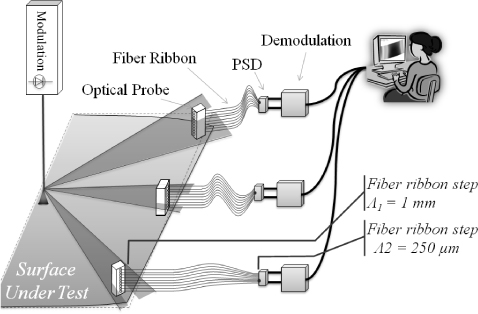
A prototype sensor has been realized to demonstrate the feasibility of this principle. A 100 mW laser diode at 980 nm generates a 5 mm reference plane obtained after reflection on an axicon mirror placed in the centre of the studied area. Each probe consists of a network of 40 fibers spaced by 1 mm (core diameter 50 μm). At the other end, fibers are spaced by 250 microns to illuminate a 12 mm PSD. The measurement of the barycenter of the light distribution at the output of the ribbon provides a resolution better than 100 μs despite the 250 μm spacing between each fiber.
It is also possible to use CCDs for an equivalent resolution. The analogical device is cheaper but the digital device avoids time drift, which is mandatory to ensure the radiation pattern remains unchanged throughout the life of the radar system.
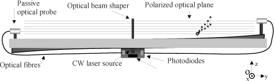
The second solution is very promising but has a lower maturity level [LES 09a]. In this case, the optical reference is thick and the state of polarization shifts linearly with height. Thus the space above the radiating surface is fully encoded through polarization. Intercepted light is analyzed through a birefringent cube placed in front of two optical fibers that deport the photo-detection below the surface. The setup is shown in Figure 15.8.
Figure 15.8. Polarimetric sensor principle
A 1D preliminary experiment was conducted (Figure 15.9). A progressive rotation of the linear polarization state is then obtained using the circular anisotropy (also called optical activity) of a crystalline quartz prism [HUA 97]. The optical activity introduces polarization rotation while keeping the polarization state linear. This prism is cut with the optical axis perpendicular to the entrance facet. A second prism made of amorphous glass is glued top-to-bottom with the quartz-prism to avoid any unwanted refraction deviation.
Figure 15.9. Experimental setup for the measurement of the polarized plane
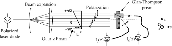
After the two prisms, the polarization of the incident light undergoes a rotation angle α depending on the z position:
[15.5] ![]()
Δn, the refraction index difference, is related to the optical activity of the quartz. Δn ~ 4.8×10⁻⁵
In the experiment described in the Figure 15.9, the analysis of the polarization state gives as z the position of the probe into the optical reference plane. The Glan-Thompson-type polarization splitter cube splits the incident polarization into two orthogonal polarization states and changes the polarization information into intensity. At the ends of the ribbon, intensities are:
[15.6] 
where Ix/z (z) is the analyzed intensity for the polarization axis x and z. Ratio measurement (IZ−IX)/(IX + IZ) gives the wanted position z.
15.4. Compensation with knowledge of the antenna shape
Once the position of all radiating elements is known, we have to compute a compensation law to restore an acceptable radiation pattern. Array synthesis methods can find the ideal excitation law for a specific radiation pattern. These methods are attractive because they can guarantee a template and thus a pointing accuracy and side lobe level. However, all these methods are inherently iterative and need a convergence criterion. This section is dedicated to direct compensation methods based on a variational criterion.
In the first part, we present the basic compensation corresponding to the simple re-phasing of the signals. Then we will study a compensation method acting on an extended angular range of the radiation pattern.
All the presented methods are applicable to a 2D array. Out of concern for clarity, we present formulas for a linear antenna. Figure 15.10 shows the S-band antenna used to illustrate this section.
Figure 15.10. 27 element linear antenna
The antenna consists of 27 regularly spaced elements d=0.6λ. We observe the “sum” radiation pattern and the desired pointing direction u0 is chosen at −20°.
15.4.1. Phase compensation in the main direction
It is essential to know the initial excitation law and the desired pointing direction to establish direct compensation. The first implementation aims to recover the main lobe. It is important to notice that a spatial displacement corresponds to a physical delay and can only be compensate by a phase shift in a single direction.
The array factor for a perturbed linear array deformed along (Oz) pointing in the direction u0 is given by the following equation:
[15.7] ![]()
The principle of the basic compensation is to change the excitation law, adding to each radiating element a phase term corresponding to the perturbation in the pointing direction. Letting g be the compensation excitation law, we have:
[15.8] 
The compensated array factor is then:
[15.9] ![]()
Equation [15.9] clearly shows that the compensated array factor is equal to the ideal array factor around the pointing direction u = u0.
We apply this formula to the deformations presented in the first section. Figure 15.11 compares the radiation patterns of an antenna with the even deformation, with and without compensation.
Figure 15.11. Radiation pattern with and without compensation — (inset) even deformation
The main lobe is fully recovered; the 3 dB width is identical to the ideal case of the non-deformed antenna. However, the compensation becomes less effective around the main lobe. To illustrate this phenomenon, observe the diagram for a randomly deformed antenna. The maximum amplitude is λ/5. Figure 15.12 shows the different radiation patterns (ideal, disturbed and compensated).
Figure 15.12. Radiation pattern with and without compensation — (inset) random deformation
Figure 15.12 shows that even if the main lobe is not affected, the side lobes are still strong at -20 dB. This compensation is efficient to recover the main lobe and the first side lobes. Thanks to its extreme simplicity, this compensation should be sufficient for many systems.
In the next section, we will focus on a compensation algorithm that will significantly improve the results of Figure 15.12.
15.4.2. Compensation by spectral analysis of deformations
The radiation pattern of an M element antenna has M degrees of freedom. We can therefore choose the amplitude of the M diagram in independent directions [LES 09b, WOO 47]. Based on spectral analysis of the deformation, the demonstration is being conducted for a linear antenna deformed along the axis (Oz). This method is extensible to 2D antennas and positioning defects in x, y and z.
A Fourier analysis shows that the array factor can be written as the sum of elementary patterns in different directions. Assuming small deformations, we then show that the array factor of a perturbed array can also be decomposed. Perturbation in the array factor can be written as a perturbation of the excitation law.
15.4.2.1. Expression of the ideal array factor
Without positioning errors, the array factor of an ideal antenna is a periodic function over ° λ/2d:
[15.10] ![]()
This array factor is a sum of unitary array factors centered in all the controllable directions. To obtain the desired formulation, we perform a Fourier transform of excitation coefficients. The Fourier transform operators adapted to our formalism are:
[15.11] ![]()
[15.12] ![]()
If σ = FFT (f), then by reversing the sum symbols, the array factor of the antenna can be written:
[15.13] ![]()
[15.14] 
The array factor is expressed as the weighted sum of unitary patterns. If U(u) is a unitary pattern, we have finally:
[15.15] ![]()
Each array factor U is steered on a different angle. Figure 15.13 represents all the main lobes of these functions.
Figure 15.13. Representations of orthogonal beams (up to the first zeros) for a 27 element linear antenna
Figure 15.14 shows two adjacent orthogonal beams (p = 0 and p = 1). It illustrates the orthogonal properties of the beams. They all reach their maximum for angles where other beams are null.
Figure 15.14. Two successive orthogonal beams (p=0, p=1)
Orthogonal property enables us to control all directions independently. However, grating lobes limits compensation. Figure 15.15 shows two orthogonal beams for p = 0 and p = 12.
Figure 15.15. Compensation out of periodicity domain
Beams near the periodicity boundary reveal grating lobes spaced by λ/d. The direction of the maxima is obtained by equation [15.15]:
[15.16] ![]()
Finally, the ideal array factor takes the following shape:
[15.17] ![]()
15.4.2.2. Factor expression deformed network
The perturbed array factor cannot be written directly as the sum of independent beams. Under the hypothesis of small displacements, we can write:
[15.18] 
It is imperative to write the perturbation as a sum of orthogonal beams. By introducing ρz, the perturbation term is then:
[15.19] 
The perturbation part F1 is now expressed as a sum of elementary functions U.
[15.20] ![]()
The expression is similar to equation [15.17], but the directional vector factorizes the perturbation. It is not possible to directly apply the inverse FFT to return to the excitation laws space. However, the function U(u+up) has a maximum in the direction u = up, apart from this direction, the function is low (side lobes at -13.2 dB, Figure 15.16).
Figure 15.16. For each U function the maximum is reached at up
For each component p and for the perturbation only, we will assimilate the direction function u to the unique direction up. Then we can write the perturbation as a sum of orthogonal beams:
[15.21] ![]()
Returning to the complete expression of the array factor of the deformed antenna, we can write:
[15.22] 
Finally, we can return to the excitation laws space:
[15.23] 
The array factor of the deformed antenna is written as an ideal array factor with a perturbation of its excitation law on each of the radiating elements. Noting that γ and g are imaginary, we can express the term g as a phase perturbation only:
[15.24] ![]()
Finally, the phase perturbation is:
[15.25] ![]()
Obviously, compensation of the deformation is obtained by applying the opposite phase of equation [15.25] on each of the radiating elements. This expression directly links, by a simple calculation, the deformation measurements to the compensation phase law. To illustrate the compensation of the radiation pattern, Figure 15.17 plots the radiation pattern of the antenna witnessing the random deformation.
Figure 15.17. Radiation pattern with and without compensation — (inset) random deformation
Compensation is efficient throughout the periodicity domain. Beyond this, lobes are higher. Figure 15.15 shows that for the orthogonal beams focused on an angle up, a lobe centered on up-λ/d appears. Knowing this physical limitation, it is imperative:
– either to ensure that the average level of these raising lobes is as low as possible. In this case, the level of these lobes will limit the maximum deflection of the antenna;
– or to decrease the spacing between elements to spread the periodicity domain over the field of view of the antenna.
Compensation based on the spectral analysis of deformations gives excellent results if the spectral components of the deformation have a magnitude much smaller than the wavelength.
15.5. Experimentation on a deformable antenna mock-up
The deformable antenna mock-up (Figure 15.18) simulates the behavior of a real antenna structure. It is instrumented with the fiber ribbon sensor.
Figure 15.18. Drawing of the deformable antenna mock-up
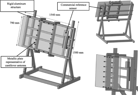
Figure 15.19. Photograph of the instrumented mock-up
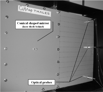
Once positions of the radiating elements are known, it is possible to calculate the compensation law. Figures 15.20 and 15.21 show the computer program for the acquisition, signal processing and real-time shape display. We can see radiation patterns with and without compensation. For illustration purpose, we have simulated a linear antenna composed of 40 elements placed at the end of the structure, subject to deformation [LES 09c].
Figure 15.20. Even deformation: (a) antenna shape display; (b) uncompensated pattern; (c) compensated pattern

Figure 15.21. Odd deformation: (a) antenna shape display; (b) uncompensated pattern; (c) compensated pattern
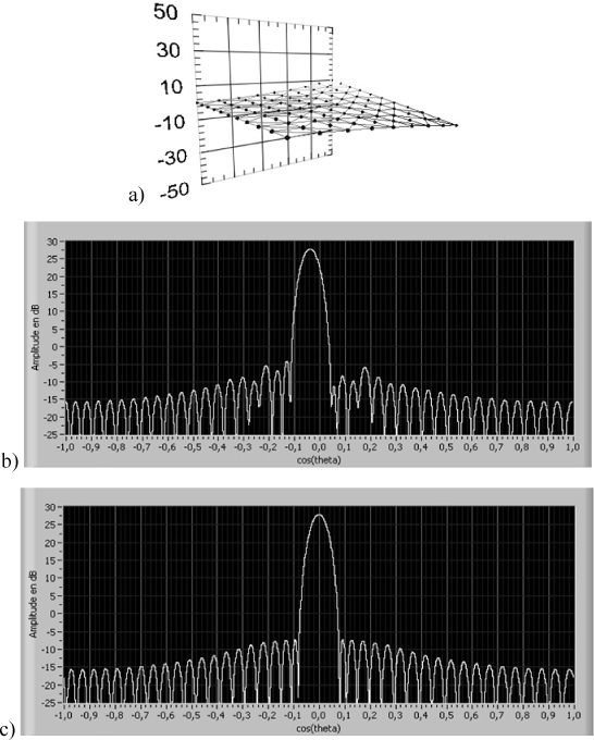
We can see that in these two distinct cases, a good knowledge of the antenna shape allows us to compensate the radiation pattern and make it very close to the non-deformed antenna pattern.
15.6. Conclusion
In this study, we have characterized mechanical deformations of array antennas and developed a method to compensate their radiation pattern. The compensation system was developed from analysis to the first experiments on a representative mock-up of a radar antenna structure in the S-band.
Mechanical perturbations are non-stationary according to the pointing direction and evolve dynamically according to external conditions. Changing the shape of the antenna causes a beam squint and a strong increase of the side lobes. The largest deformations result in lower gain. Perturbations of the antenna shape causes an error of several degrees on the angular location of targets and dynamic shifts are adding substantial bias in the measurement of target velocity.
Instrumented methods appear to be flexible to any kind of high-directivity antennas. The sensors developed in these studies are adaptable to the objectives set in terms of bandwidth, dynamic range and resolution. The fiber ribbon sensor is based on a very simple physical principle and gives an absolute position measurement. The sensor based on polarization measurement requires more development to become fully operational for deformable antennas, but production cost is the same regardless of the number of local probes. These sensors are suitable for electronic scanning antennas of different sizes and operating in other frequency bands.
To make these non-standard antennas completely operational, we must take into account the effects of rotation and translation of the whole antenna, including the twisting of the mast support. Sensors measuring the overall misalignment of the antenna are needed. Methods developed here can easily take into account information from other sensors, and steer the beam in the right direction.
Finally, only an instrumented deformable antenna demonstrator will provide clear evidence on the applicability of this method. The ability to detect and estimate target radial velocity through a deformable antenna will be the focus of future demonstrations.
15.7. Bibliography
[CHE 89] LE CHEVALIER F., Principes de traitement des signaux radar et sonar, Masson, 1989.
[HUA 97] HUARD S., Polarization of Light, John Wiley & Sons, New York, 1997.
[JAS 61] JASIK H., Antenna Engineering Handbook, McGraw Hill, 1961.
[LES 08] LESUEUR G., GILLES H., GIRARD S., MERLET T., QUEGUINER M., “Optical sensor for real time reconstruction of distortions on electronically steered antenna”, IEEE Photonics Technology Letters, vol. 20, no. 21, pp. 1763–1765, 1 November 2008.
[LES 09a] LESUEUR G., MARCINIAK A., GILLES H., GIRARD S., MERLET T.H., QUEGUINER M., “Polarization optical sensor for dynamical deformation measurements on 1D or 2D mechanical structures”, IEEE Photonics Technology Letters, vol. 21, no. 18, pp. 1311–1313, September 2009.
[LES 09b] LESUEUR G., CAER D., MERLET T.H., GRANGER P., “Active compensation techniques for deformable phased array antenna”, Conference on Antenna and Propagation Eucap, Berlin, Germany, March 2009.
[LES 09c] LESUEUR G., MERLET T.H., QUEGUINER M., GRANGER P., RENAULT F., GILLES H., GIRARD S., “Management of deformable active antenna”, International Conference on Radar, Bordeaux, France, October 2009.
[SCH 07] SCHIPPERS H. et al. “Vibrating antennas and compensation techniques research in NATO/RTO/SET 087/RTG 50”, IEEE Aerospace Conference, Big Sky, Montana, USA, March 2007.
[WOO 93] WOODWARD P.M., “A method of calculating the field over a plane aperture required to produce a given polar diagram”, J. IEE, vol. 93, pp. 1554–1558, 1947.
1 Chapter written by Guillaume LESUEUR.