
Chapter 20
Vector Spherical Harmonic Modeling of
3D-antenna Radiation Function
for an UWB-RT Simulator1
20.1. Introduction
The development of communications and ultra-wideband (UWB) localization systems has given rise to applications requiring more realistic reconstructions of signals transmitted between two terminals. In this situation of realistic signals, taking into account antenna effects (considering frequency and polarization aspects) is essential in order to provide not only realistic waveform characteristics, but also realistic signal received power. However, this necessity of considering antenna radiation pattern accurate information leads to large data volumes which are difficult to handle. Furthermore, this problem raises a significant question: what is the best approach in order to make both a description and quickly reconstruct the antenna radiation function in arbitrary directions?
This question served as the starting point of this study, whose purpose was to find an efficient manner of introducing antenna behavior into ray tracing (RT) channel modeling tools. Vector spherical harmonic (VSH) expansions of antenna radiation function are proposed here as a solution for both issues: compression of the amount of data needed for describing antenna characteristics and fast and correct retrieval of antenna array responses for waves coming from arbitrary directions. The presented approach stands at an intermediate level between the exact electromagnetic simulation and the use of a scalar radiation pattern in a simplified manner. It has been constructed under the assumption that antenna and propagation models can be separated into two distinct parts.
The idea of exploiting spherical harmonics in antenna context is not completely new; it was initially proposed by Christophe Roblin and Alain Sibille [ROB 08]. We extend this idea by proposing a specific implementation for RT tools. Also, VSH were lately used in the field of channel modeling by Del Galdo [DEL 06].
Section 20.2 of this study presents the principle and the adopted notation for the RT code. Section 20.3 describes the formalism of VSH decomposition applied to two antennas: a classical dipole antenna inclined at a 45° angle from the z axis of its local coordinate system and a UWB monocone antenna developed at CEA-Leti [BOU 07]. Section 20.4 shows the implementation of the above described antennas in modeling UWB propagation channel transfer function, using their VSH coefficients.
20.2. Deterministic channel model based on ray tracing
This first section presents the mathematical formalism for an RT based propagation simulator [LOS 06], [STU 06], [SUG 04], [YAO 03] with realistic antenna behavior. This formalism uses general principles and notations presented in [AUB 06].
20.2.1. PyRay channel simulation tool
PyRay channel simulation tool is build up at IETR. This simulator aims to model radio propagation channel for multi-standard systems and/or UWB. It is mainly used in indoor environments, although its use could be extended to outdoor applications. PyRay tool follows a continued development progress, evolving towards a heterogeneous radio simulation platform, that will integrate the mobility of radio nodes which is relevant in different application areas, such as localization.
20.2.1.1. Simulator architecture
PyRay code is designed in order to take into account all electromagnetic waves propagation effects (transmission, specular reflection, refraction and diffraction), material properties for all elements inside the building, terminals mobility, UWB antenna patterns and multiple-antenna arrays at transmitter and/or receiver ends.
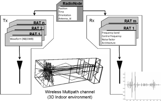
Figure 20.1. PyRay simulator architecture
PyRay channel simulator uses scientific packages of Python programming language [TRA 07], including numpy, scipy [SCI 10] and matplotlib. Working with dynamic object-oriented programming languages such as Python and C/C++ offers the ability to better manage tool complexity and to define data objects denoting basic elements of the radio scene.
The channel simulator is broken down into three major blocks as shown in Figure 20.1: transmitter Tx, wireless multipath channel and receiver Rx. Several classes like RadioNode and RadioLink have been introduced.
RadioNode class denotes either a transmitter, or a receiver. For each radio access node, this class defines its temporal and spatial coordinates, its associated radio access technology (RAT) and its specific antenna type and orientation. This class was introduced to provide specific parameters for the transmitter and receiver.
RadioLink class describes the propagation channel between a transmitter and a receiver. The propagation channel is computed through one RT simulation over a large spectral bandwidth, using geometrical optics (GO) and uniform theory of diffraction (UTD). Angular information, attenuation and delay are accessible from this class.
PyRay code is particularly well-suited for developing and testing various transceiver architectures, using different RATs.
20.2.1.2. Propagation channel – ray tracing
After a detailed 3D description of the environment in which the simulation will be performed, including constituent materials and transmitter and receiver positions, the RT simulator calculates propagation delays, angles of departure (AoD) and angles of arrival (AoA) for all propagation paths and all frequency points.
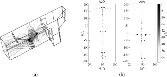
Figure 20.2a shows the most important 3D rays obtained with PyRay RT based-transmission channel simulation tools in a typical indoor environment. The transmitter is located at (2,1,1.2)m and the receiver is located at (8,3,1.8)m in a line of sight (LOS) configuration between Tx and Rx. The corresponding AoA/AoD diagram is depicted in Figure 20.2b. These figures show that only a few directions (θk,ϕk) need to be computed for a given radio link.
Figure 20.2. Example of RT (a) and the associated AoA/AoD diagram (b)
Rays contributions in received signal are individually considered, which is relevant in facilitating information access (AoD, AoA, interaction type) at any time. In addition, any received signal may be reconstructed from a very sparsely sampled propagation dyad that can be stored once for all and later exploited for any radio standard waveform occupying various bandwidths and passing to various arbitrarily oriented antennas.
20.2.1.3. Transmission channel
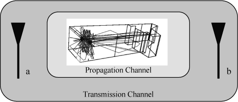
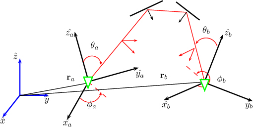
A transmission channel refers to a couple of transmitter/receiver antenna and to the propagation channel which links both antennas (Figure 20.3). In this context, “a ” is the transmission antenna and “b ” is the reception antenna. The transmission channel strongly depends on its antennas radiation patterns.
Figure 20.3. Transmission channel
Each ray k is characterized by a free space propagation delay τk along its length and by a complex matrix ![]() which stands for physical effects that rays go through, for the divergence factor and for delay that exceeds free-space propagation and transmission and reception antenna. The symbol “ ~ ” expresses the propagation delay that was not considered in channel transfer function.
which stands for physical effects that rays go through, for the divergence factor and for delay that exceeds free-space propagation and transmission and reception antenna. The symbol “ ~ ” expresses the propagation delay that was not considered in channel transfer function. ![]() is obtained from the combination of a ray propagation dyad
is obtained from the combination of a ray propagation dyad ![]() and two vectors associated with both antennas:
and two vectors associated with both antennas:
[20.1] ![]()
[20.2] 
In previous formulations, the channel matrix is expressed in antenna local bases (as indices suggest). ![]() matrix is obtained from the pre-calculated matrix
matrix is obtained from the pre-calculated matrix ![]() expressed in global coordinate system and from rotation matrices depending on the arbitrary orientation of transmission and reception antennas.
expressed in global coordinate system and from rotation matrices depending on the arbitrary orientation of transmission and reception antennas.
In equation [20.1], the two vector functions ![]() , evaluated for the k-th ray direction, model antenna radiation behavior.
, evaluated for the k-th ray direction, model antenna radiation behavior.
Figure 20.4. Details of geometric model
20.2.1.4. Method for received signal reconstruction
For IR-UWB (impulse radio-ultra-wideband) signal applications, the signal r(τ) at the output of the receiving antenna can be expressed as a summation over the whole set of rays:
[20.3] ![]()
where τk is the propagation delay corresponding to free space propagation along total length of the k-th ray and:
[20.4] ![]()
In [20.4]:
– IFT is the inverse Fourier transform;
– Nray is the total number of rays;
– Wγ (f) is the corresponding spectrum of the modified signal waveform transmitted by the emission antenna “a ”.
The modified signal waveform includes all rays common factor γab(f), expressing the integration impact due to the reception antenna mechanism, as follows:
[20.5] ![]()
The received signal is obtained by summing up each ray contribution with is proper free space propagation delay, as depicted in Figure 20.5.
Figure 20.5. Received signal construction
20.2.2. Antenna related issues
Until now, complete antenna characterization can be easily carried out by electromagnetic simulation or through near-field measurement.
In a 3D-RT, all ray directions of departure or arrival may occur. This leads to the necessity of describing antenna vector function F(f,θϕ) over the full 4π steradians and the frequency band of interest. For wideband frequency applications, this leads to a large amount of data that is required to be stored. In addition, extracting antenna functions in particular directions for estimating specific transmission channels involves interpolation processes and makes data difficult to exploit.
Let us consider the example of an antenna operating in 2 GHz to 8 GHz frequency band. For a frequency step of 50 MHz and a spatial resolution of 5°, 121 radiation patterns of 72 points in azimuth (ϕ) and 37 points in elevation (θ) are required in order to get a complete detailed description of this antenna. Furthermore, this leads to 2 × 2,664 × 121 = 644,688 complex arrays of 64 bit precision floating point numbers, loaded into a 5 Mb file size.
A trivial approach in RT simulation tools consists of firstly extracting F(f,θk,ϕk) function only in some specific directions (θk,ϕk) along AoD and then calculating F(f,θk,ϕk) through interpolation in each k-th ray direction. This computer task is even more complex and time consuming if antenna stored file is large. Anyway, it can only be used to approximate the real values of antenna function.
In this chapter, we will propose an alternative method to the described approach, based on VSH expansion [HIL 54] of the antenna radiation function. The proposed method not only allows efficient data access and good compression factor, but also fast reconstruction of antenna radiation function for arbitrary directions.
20.3. Antenna vector function description via VSH
The VSH method is already largely used in different fields like meteorology, chemistry, acoustics, image processing and mathematical physics applications. It will be applied here for modeling antenna vector fields in the IR-UWB RT simulator.
Spherical harmonics are similar to Fourier transforms (FT), in 1D higher on the sphere. VSH form a basis of orthogonal functions out of which we can describe an arbitrary vector function on the surface of a sphere.
VSH transform establishes a one-to-one correspondence between spherical vector function and a series of complex coefficients. The use we make of it reveals two distinct steps:
– The analysis step, which consists of generating the complex VSH coefficients corresponding to the orthogonal basis. The coefficients are generated accessing free Spherepack packages [ADA 97] of Fortran through Python. This step is done offline and only once for each particular antenna.
– The synthesis step (the reverse process to the previous one), which is to build up, as quickly as possible, the antenna vector function and only in a specific set of directions corresponding to AoD/AoA coming out from the RT engine.
20.3.1. VSH analysis step
This phase aims to calculate the VSH expansion coefficient set associated with the antenna vector function F(f,θ,ϕ) for which a complete spatial and frequency description is available. The analytical expression of VSH coefficients obtained by projecting on the orthogonal basis is given by [ADA 97]:
[20.6] 
[20.7] 
[20.8] 
[20.9] 
[20.10] ![]()
In previous equations (from [20.6] to [20.10]), the integer index n and m are referred as the degree (n ∈ N ) and the mode (m ∈ [-n,n]) of the VSH expansion.
The n index labels colatitude (elevation), while the m index labels longitude (azimuth).
Calculation of ![]() and
and ![]() real functions will be detailed in section 20.3.2.
real functions will be detailed in section 20.3.2.
For implementation, we call the vha function of Spherepack library [ADA 97] twice successively: once for real part ℜ{F(f,θ,ϕ}and once for the imaginary part ℑ{F(f, θ, ϕ) of F(f,θ,ϕ). For each vha function call, a set of 8 real coefficients is created. They are then recombined in order to build up the 4 VSH complex coefficients ![]() , according to Figure 20.6.
, according to Figure 20.6.
Figure 20.6. Construction of VSH coefficients
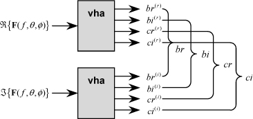
Figure 20.7 describes the structure of the matrix of VSH coefficients for a particular frequency and for a particular VSH expansion order N = 4. If considering 0 ≤ n ≤ N and −n ≤ m ≤ n, the number of coefficients needed to achieve an N-order VSH transform is (N+1)2 (Figure 20.7a). However, since the matrix is symmetric it may be generated only for 0 ≤ n ≤ N and 0 ≤ m ≤ n as shown in Figure 20.7b. This change will act to decrease the number of VSH coefficients to (N+1)(N+2)/2.
The 4 VSH coefficients ![]() are calculated for each frequency point. At this stage, the coefficients are represented by a 3D-array matrix format (f × n × m), as shown in Figure 20.8a. For ease of synthesis, it is convenient to reduce it to a 2D-array matrix format (f × k) (Figure 20.8b) by introducing the index k, defined by a specific trajectory in coefficient space (increasing n, increasing m for each n) (Figure 20.7).
are calculated for each frequency point. At this stage, the coefficients are represented by a 3D-array matrix format (f × n × m), as shown in Figure 20.8a. For ease of synthesis, it is convenient to reduce it to a 2D-array matrix format (f × k) (Figure 20.8b) by introducing the index k, defined by a specific trajectory in coefficient space (increasing n, increasing m for each n) (Figure 20.7).
Figure 20.7. VSH coefficient matrix for N = 4
New coefficient index k which replaces an (m,n) couple is defined as:
[20.11] ![]()
Converse relations for each k to have one (m,n) couple are given by [20.12] and illustrated in Figure 20.8c for the first indexes.
[20.12] 
Figure 20.8. Structure of VSH coefficients matrix; a) 3D format, b) 2D format, c) (n, m) couple via k index
VSH analysis requires significant computational time. However, this operation is performed only once for each particular antenna and remains available for field reconstruction in any direction.
20.3.2. Calculation of VSH basis (V and W)
VSH basis ![]() are well defined functions, depending on the spherical coordinate θ and being derived from associated Legendre functions of the first kind
are well defined functions, depending on the spherical coordinate θ and being derived from associated Legendre functions of the first kind ![]() :
:
[20.13] 
Since the norm of the associated Legendre functions increases with the degree n, we must “normalize ” the spherical harmonics. The normalization of ![]() and
and ![]() resumes to the next formulas:
resumes to the next formulas:
[20.14] 
[20.15] ![]()
In the adopted notation, normalization is expressed by the notation “–” ![]() .
.
20.3.3. VSH synthesis step
VSH synthesis consists of rebuilding antenna vector function F(f,θ , ϕ) from its VSH set of complex coefficients (brk,bik,crk,cik), using the next equations:
[20.16] 
For m symmetry reasons, it is convenient to isolate the term m = 0 of the summation [20.16]:
[20.17] 
where:
[20.18] 
Synthesis relations are useful in the quick retrieval of F(f,θ , ϕ) in specified directions (θk, ϕk). The choice of the order N of VSH decomposition is related to the dimensions of the antenna and to its operating frequency [BUC 87]. Important angular variations of antenna radiation pattern lead to high N values.
Unlike VSH analysis, synthesis only uses simple operations and is therefore not very time consuming.
20.3.4. VSH expansion example
This section deals with two examples of VSH expansion, applied to both UWB antennas shown in Figures 20.9 and 20.10: a wire dipole antenna simulated on NECTM and a monocone antenna simulated on HFSSTM. Antenna radiation patterns are obtained for 2 GHz to 8 GHz frequency band with 50 MHz frequency step and 5° spatial resolution. Thus, for one frequency value, antennas are described with 2,664 complex arrays (5,328 complex scalars).
Figure 20.9. Dipole antenna (dimension 2.66 cm) and corresponding power radiation pattern at 4 GHz
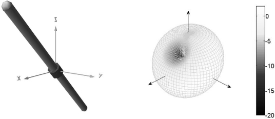
Figure 20.10. Monocone antenna and corresponding power radiation pattern at 4 GHz
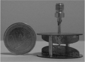
Figure 20.11. VSH coefficient absolute values in dB at 4GHz, as a function of degree n and mode m for dipole antenna (a) and (b) monocone antenna
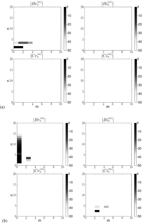
Figure 20.12. Evaluation of dipole antenna vector function reconstruction at 4 GHz with all VSH coefficients: module (a), phase (b)
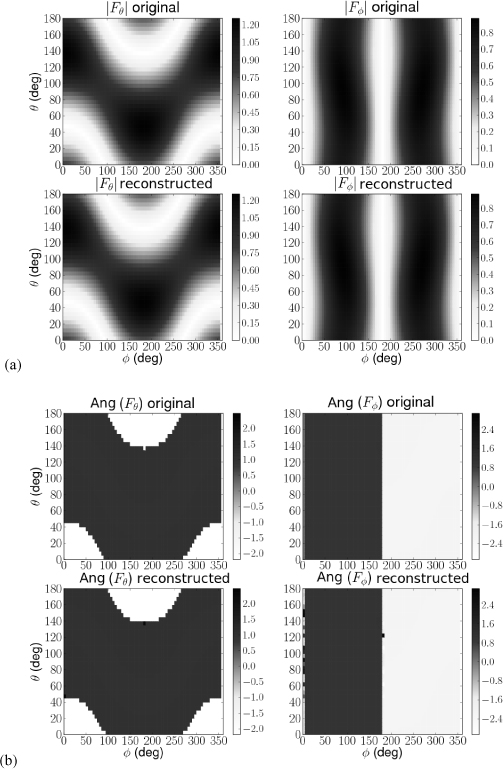
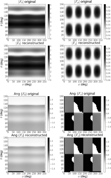
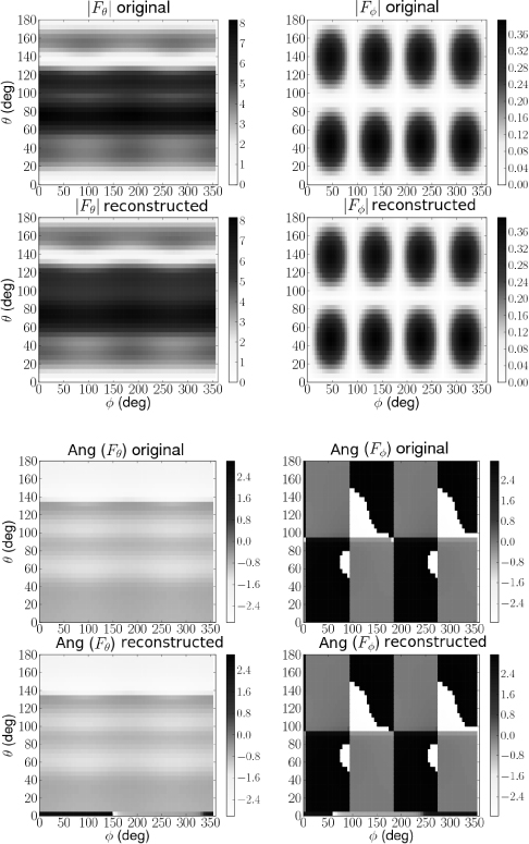
Figure 20.13. Evaluation of monocone antenna vector function reconstruction at 4 GHz with all VSH coefficients: module (a), phase (b)
VSH expansion is firstly applied to the simulated antenna radiation patterns at 4 GHz. Figure 20.11 shows the normalized absolute values (in dB) of the corresponding VSH coefficients, as a function of degree n and mode m up to order 20. In Figure 20.11a, it is obvious that for the dipole antenna, most significant coefficients have n≤4 and m≤3. This small number of coefficients may be explained by the fact that dipole antenna has a simple radiation pattern, without any important angular variations (Figure 20.9). In the case of monocone antenna significant coefficients have higher degree n≤15 (reflecting important variation of radiation pattern in elevation) and m = 0 (reflecting an omnidirectional behavior in azimuth).
Figures 20.12 and 20.13 present the original radiation pattern for both antennas and the corresponding synthesized ones through VSH method. Note that VSH synthesis has proved a proper reconstruction of antenna radiation pattern.
20.3.5. Data compression for antenna data storage
Figure 20.11 points out that the number of significant coefficients that need to be computed for VSH synthesis at a particular frequency is low. This is particularly interesting when the VSH synthesis is carried out for a wide frequency band. So let us now apply the VSH expansion to the simulated antenna radiation patterns for all frequency bands (2-8 GHz, each 50 MHz).
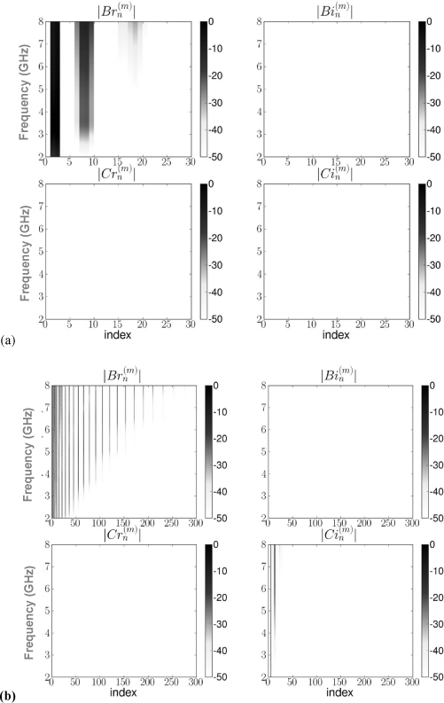
Figure 20.14 displays the normalized absolute values (in dB) of the corresponding VSH coefficients, as a function of index k and frequency f. It shows that the number of important VSH coefficients is gradually increasing with frequency. According to Figure 20.14, for a dipole antenna, coefficients may be neglected for k>21. For a monocone antenna, they may be neglected for k>277. Nevertheless, we can also note that for many index k, VSH coefficients are negligible over the entire considered frequency band.
For the purpose of reducing data for storage, VSH synthesis of antenna vector function can be limited to the essential coefficients. The criteria used to identify these coefficients are:
– an energy criterion on coefficients: calculation of energy for each coefficient group ![]() is performed for each index k over the entire frequency band.
is performed for each index k over the entire frequency band.
– an error criterion on radiation patterns: calculation of mean square error (MSE) between synthesized antenna functions and original ones is done over the entire frequency band.
Figure 20.14. VSH coefficient absolute values in dB as a function of index k and frequency f for both UWB antennas: (a) dipole; (b) monocone
In order to estimate performances of VSH expansion, Figure 20.15 shows the relative MSE on each studied antenna radiation pattern and for both polarizations, as a function of index k of coefficients used for VSH synthesis. While computational time is directly proportional to k, error increases with the decrease of k. As shown in Figure 20.15, MSE≤5% corresponds to k≥5 for dipole antenna, respectively to k≥18 for monocone antenna.
Figure 20.15. Reconstruction error between VSH synthesized antenna radiation pattern and original simulated one as a function of the VSH coefficient number: (a) dipole, (b) monocone
Ultimately, with the proposed optimization technique, the antenna radiation pattern is reconstructed without many errors and with fewer VSH coefficients:
– for dipole antenna: the amount of data necessary to describe antenna is divided by 266 (from 5328 to 20 complex data), with an error equal to 3.85% on Fθ (f,θ,ϕ) and 4% on Fϕ (f,θ,ϕ). Time required for VSH synthesis is 1.01 seconds on an Intel Core 2 6000 @2.4GHz with 3.2 GB RAM.
– for a monocone antenna: the amount of data necessary to describe the antenna is divided by 74 (from 5,328 to 72 complex data), with an error equal to 4.67% on Fθ (f,θ,ϕ) and 1.19% on Fϕ (f,θ,ϕ). Time required for VSH synthesis is 1.22 seconds.
In order to estimate performances of VSH expansion, the antenna complex vector radiation pattern is reconstructed with the most significant coefficients and it is then compared to the original simulated pattern. Figures 20.16 and 20.17 illustrate the evaluation (after minimizing coefficient number) for each reconstructed component of the antenna vector function at 4 GHz (dipole in Figure 20.16 and monocone in Figure 20.17). As can be seen, antenna radiation pattern is faithfully reconstructed.
Figure 20.16. Evaluation of dipole antenna vector function reconstruction at 4 GHz with minimum of VSH coefficients: module (a), phase (b)
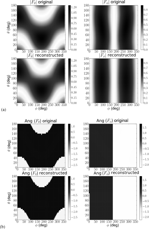
Figure 20.17. Evaluation of monocone antenna vector function reconstruction at 4 GHz with a minimum of VSH coefficients: module (a), phase (b)
20.4. Immediate RT tool application
20.4.1. Antenna vector function synthesis
This section describes the appropriate matrix formalism for RT tool implementation. In order to construct the simulated signal at the output of received antenna, we define the following matrix:
[20.19] ![]()
where:
– the operator ⊗ stands for the element wise product;
– Wγis the matrix associated with the modified transmitted waveform from antenna “a ”:
[20.20] ![]()
– ![]() is the matrix of complex amplitudes associated with all Nray rays, deduced from matrix
is the matrix of complex amplitudes associated with all Nray rays, deduced from matrix ![]() (obtained by RT simulation) and from two antennas vectors Fa,Fb (obtained by VSH synthesis, only for the particular Nray directions and Nf frequencies, given by the RT simulation). Mathematically, it may be calculated from:
(obtained by RT simulation) and from two antennas vectors Fa,Fb (obtained by VSH synthesis, only for the particular Nray directions and Nf frequencies, given by the RT simulation). Mathematically, it may be calculated from:
[20.21] ![]()
In formula [20.21]:
– ![]() are 4 (Nf ×Nray) matrices, associated with each term of
are 4 (Nf ×Nray) matrices, associated with each term of ![]()
– ![]() are 4 (Nf ×Nray) matrices, associated with each term of Fa, Fb describing receiver, and respectively transmitter antenna behavior for all Nray rays and for all Nf frequency points. They are given by the [20.22] system of equations:
are 4 (Nf ×Nray) matrices, associated with each term of Fa, Fb describing receiver, and respectively transmitter antenna behavior for all Nray rays and for all Nf frequency points. They are given by the [20.22] system of equations:
[20.22] 
In the [20.22] formulas:
– Br, Bi, Cr, Ci are 4 matrices (Nf ×Nk) of VSH coefficients;
– ![]() represent real and imaginary parts of two complex matrices
represent real and imaginary parts of two complex matrices ![]() , called matrices of VSH transform basis.
, called matrices of VSH transform basis. ![]() and
and ![]() are deduced from
are deduced from ![]() matrix (associated with
matrix (associated with ![]() and
and ![]() terms) and from complex exponential matrix E (associated with ejmϕterm):
terms) and from complex exponential matrix E (associated with ejmϕterm):
[20.23] ![]()
NOTE: For practical implementation of antenna vector functions VSH synthesis for specified directions and frequency values, we have adopted a new notation, in order to avoid possible confusion between matrices of VSH coefficients and matrices of VSH transform basis. Consequently, in formula [20.21], V and W are identified with B and C defined in [ADA 97].
The matrix R (from [20.19]) can equally be used for the construction of received signal either in the frequency domain, or in the time domain, by introducing each ray’s phase shifts or delays. When working with temporal domain reconstruction scheme, each matrix column that corresponds to each ray must be extended by forcing Hermitian symmetry, before applying the IFT. The received signal is reconstructed as a superposition of all rays after introducing their proper delays xk.
20.4.2. Application to IR-UWB signals
This section presents some simulation results obtained from the PyRay simulation tool. This tool implementation is based on the matrix formalism described in section 20.4.1.
The following illustrations are all made in the indoor environment described in Figure 20.2a, where the main rays are also depicted. The transfer function of the propagation channel has been simulated over a wide frequency range from 2 to 11 GHz. For this application, only the 3.5 to 6.5 GHz band is used. The transmitted waveform is a normalized impulse, generated for: fc = 5 GHz, B10dB = 3 GHz and it is plotted in Figure 20.18. The positions of the transmitter Tx and receiver Rx correspond to a LOS distance of dLOS = 6.35 m, equivalent to a delay of τLOS = 21.17 ns.
Figure 20.18. Transmitted pulse signal
This study focuses on evaluating the impacts and performances of realistic antenna behavior in the proposed deterministic simulation tool, for different configurations: a couple of dipole antennas and a couple of monocone antennas. These antennas were both presented in previous section. Identical antennas are considered for both emission and reception side. Antennas vector functions are synthesized for AoA and AoD directions shown in Figure 20.2b. For comparison purposes, simulations are also performed by replacing antenna functions by the projection of electrical field along the ![]() direction, which means simulating a vertically polarized antenna, with an omni-directional pattern in azimuth and a unity gain. We denote this model by omni. The notation “^” expresses a unitary vector quantity.
direction, which means simulating a vertically polarized antenna, with an omni-directional pattern in azimuth and a unity gain. We denote this model by omni. The notation “^” expresses a unitary vector quantity.
Figure 20.19 renders the received simulated signal for each studied configuration: omni antennas (a) dipole antennas (b) and monocone antennas (c). It should be noted here that omni antenna gain was multiplied by monocone antenna gain, so that temporal responses appear with the same order of magnitude. As a disadvantage of its orientation at 45 degrees, the dipole antenna produces a signal level much lower than the monocone antenna, which approaches the omni antenna. However, the received signals are very similar in terms of temporal distribution of energy; that was expected because it only depends on propagation channel, which is the same for the 3 considered configurations. On the other hand, there is a slight delay in dipole antenna case, certainly because dipole antenna file did not get delay compensation, as it did get the monocone antenna delay. Of course, this compensation issue is very important when dealing with localization applications for which any additional fictive delays introduced for antenna are dislikeable. This compensation is easily realized during the VSH synthesis step, using phase compensation in order to ensure that antenna operates only as a factor of distortion and amplification.
Figure 20.19. Simulated received signal obtained with: omni antenna couple (a), dipole antenna couple (b) and monocone antenna couple (c)
Analysis of these three situations underline antenna importance in a transmission channel: received signal waveform depends on antenna characteristics. Some ray directions are differently weighted by antenna vector function. This is particularly notable for dipole antennas which, because of their orientation at 45 degrees, filter out some rays.
20.5. Conclusions
This study was focused on including realistic antenna effects in IR-UWB channel simulation applications, in order to improve their realism and performances. A mathematical formalism, based on VSH expansion of antenna vector function, has been developed. VSH expansion of antenna radiation function is a solution for the dual problem of antenna data storage reduction and rapid synthesis of antenna functions only in some particular directions of interest.
The whole formalism of VSH decomposition is detailed here, being complemented by a matrix formalism which can be applied to any simulator based on RT.
The advantages of VSH expansion of antenna function are illustrated by the results obtained with PyRay simulator for dipole and monocone antennas. A proper conservation of antenna radiation properties has been demonstrated with a reconstruction error less than 5%.
The developed tool can be deployed to predict the influence on the transmission channel of different antenna characteristics, especially for localization applications. It will also be used for studying more complex systems, containing multiple antennas (MIMO multiple input multiple output) and/or requiring mobility analysis.
20.6. Bibliography
[ADA 97] ADAMS J.C., SWARZTRAUBER P.N., “SPHEREPACK 2.0: A model development facility ”, NCAR Tech. Note NCAR/TN-436-STR, 62 pp., September 1997.
[AUB 06] AUBERT L.M., UGUEN B., TCHOFFO TALOM F., “Deterministic simulation of MIMO–UWB transmission channel ”, Comptes Rendus Physique, vol. 7, pp. 751–761, September 2006.
[BOU 07] BOURTOUTIAN R., DELAVEAUD C., TOUTAIN S., “Low profile UWB shorted dipole antenna ”, IEEE Antennas and Propagation International Symposium, pp. 5729–5732, 9– 15 June 2007.
[BUC 87] BUCCI O.M., FRANCESCHETTI G., “On the spatial bandwidth of scattered fields ”, IEEE Transactions on Antennas and Propagation, vol. AP-35, no. 12, pp.1445–1455, December 1987.
[DEL 06] DEL GALDO G., LOTZE J., LANDMANN M., HAARDT M., “Modelling and manipulation of polarimetric antenna beam patterns via spherical harmonics ”, 14th European Signal Processing Conference (EUSIPCO), Florence, Italy, September 2006.
[HIL 54] HILL E.L., “The theory of vector spherical harmonics ”, American Journal of Physics, 1954.
[LOS 06] LOSTANLEN Y., GOUGEON G., BORIES S., SIBILLE A., “A deterministic indoor UWB space-variant multipath radio channel modelling to measurements on basic configurations ”, Proc. EuCAP, Nice, France, 6–10 November 2006.
[ROB 08] ROBLIN C., SIBILLE A., “Ultra compressed parametric modeling of UWB antenna measurements using symmetries ”, 29th URSI General Assembly, Chicago, USA, 10–16 August 2008.
[STU 06] STURM C., SOERGEL W., KAYSER T., WIESBECK W., “Deterministic UWB wave propagation modeling for localization applications based on 3D ray tracing ”, IEEE MTT-S International Microwave Symposium Digest, 11–16 June 2006.
[SCI 10] SCIPY COMMUNITY, SciPy reference guide, 11 September 2010.
[SUG 04] SUGAHARA H., WATANABE Y., ONO T., OKANOUE K., YAMAZAKI S., “Development and experimental evaluations of RS-2000. A propagation simulator for UWB systems ”, Conference on Ultra Wideband Systems and Technologies UWBST, 2004.
[TRA 07] TRAVIS E. O., “Python for scientific computing ”, Computing in Science Engineering, vol. 9, May-June 2007.
[YAO 03] YAO R., ZHU W., CHEN Z., “An efficient time-domain ray model for UWB indoor multipath propagation channel ”, Proceedings IEEE Global Telecommunications Conference GLOBECOM, December 2003.
1 Chapter written by Roxana BURGHELEA, Stéphane AVRILLON and Bernard UGUEN.