
3.2 Invariant measures and recurrence
3.2.1 Invariant laws and measures
3.2.1.1 Invariant laws, stationary chain, and balance equations
Let ![]() be a Markov chain with matrix
be a Markov chain with matrix ![]() , and
, and ![]() be its instantaneous laws. Then,
be its instantaneous laws. Then, ![]() solves the linear (or affine) recursion
solves the linear (or affine) recursion ![]() and, under weak continuity assumptions, can converge to some law
and, under weak continuity assumptions, can converge to some law ![]() only if
only if ![]() is a fixed point for the recursion, and hence only if
is a fixed point for the recursion, and hence only if ![]() .
.
If a law ![]() is s.t.
is s.t. ![]() , and if
, and if ![]() , then
, then
and hence, ![]() is a Markov chain with matrix
is a Markov chain with matrix ![]() and initial law
and initial law ![]() and thus has same law as
and thus has same law as ![]() . The chain is then said to be in equilibrium or stationary, and
. The chain is then said to be in equilibrium or stationary, and ![]() is said to be its invariant law or stationary distribution.
is said to be its invariant law or stationary distribution.
In order to search for an invariant law, three main steps must be followed in order.
- Solve the linear equation
 .
. - Find which solutions
 are nonnegative and nonzero. Such a solution is called an invariant measure.
 - For any such invariant measure
 , check whether
  (always true if
  is finite), and if so normalize
  to obtain an invariant law
  .
.
The linear equation ![]() for the invariant measure can be written in a number of equivalent ways, among which
for the invariant measure can be written in a number of equivalent ways, among which ![]() . It is practical to use such condensed abstract notations for the invariant measure equation, but it is important to be able to write it as a system if one wants to solve it, for instance as follows.
. It is practical to use such condensed abstract notations for the invariant measure equation, but it is important to be able to write it as a system if one wants to solve it, for instance as follows.
Global balance (or equilibrium) equations
This is the linear system
It can be interpreted as a balance equation on the graph between all which “leaves” ![]() and all which “enters”
and all which “enters” ![]() , in strict sense.
, in strict sense.
The same balance reasoning taken in wide sense yields ![]() , and we obtain this equivalent version of the invariant measure equation using that
, and we obtain this equivalent version of the invariant measure equation using that ![]() . If
. If ![]() is an invariant measure then, for every subset
is an invariant measure then, for every subset ![]() of
of ![]() , the balance equation
, the balance equation
holds for what leaves and enters it. The simple proof is left as an exercise.
As in all developed expressions for ![]() , the global balance system is in general highly coupled and is very difficult to solve. This is why the following system is of interest.
, the global balance system is in general highly coupled and is very difficult to solve. This is why the following system is of interest.
Local balance (or equilibrium) equations
This is the linear system
It can be interpreted as a balance equation on the graph between all which goes from ![]() to
to ![]() and all which goes from
and all which goes from ![]() to
to ![]() .
.
By summing over ![]() , we readily check that any solution of (3.2.5) is a solution of (3.2.4), but the converse can easily be seen to be false. This system is much less coupled and simpler to solve that the global balance, and often should be tried first, by it often has only the null solution.
, we readily check that any solution of (3.2.5) is a solution of (3.2.4), but the converse can easily be seen to be false. This system is much less coupled and simpler to solve that the global balance, and often should be tried first, by it often has only the null solution.
This system is also called the detailed balance equations, as well as the reversibility equations, and the latter terminology will be explained later.
3.2.1.2 Uniqueness, superinvariant measures, and positivity
The space of invariant measures constitutes a positive cone (without the origin).
An invariant measure ![]() is said to be unique if it is so up to a positive multiplicative constant, that is, if this space is reduced to the half-line
is said to be unique if it is so up to a positive multiplicative constant, that is, if this space is reduced to the half-line ![]() generated by
generated by ![]() . Then, if
. Then, if ![]() , then
, then ![]() is the unique invariant law or else if
is the unique invariant law or else if ![]() then there is no invariant law.
then there is no invariant law.
A measure ![]() is said to be superinvariant if
is said to be superinvariant if ![]() and
and ![]() . Note that any invariant measure is superinvariant. This notion will be helpful for the uniqueness results. We use the classic conventions for addition and multiplication in
. Note that any invariant measure is superinvariant. This notion will be helpful for the uniqueness results. We use the classic conventions for addition and multiplication in ![]() (see Section A.3.3).
(see Section A.3.3).
3.2.2 Canonical invariant measure
The strong Markov property naturally leads to decompose a Markov chain started at a recurrent state ![]() into its excursions from
into its excursions from ![]() , which are i.i.d. The number of visits to a point
, which are i.i.d. The number of visits to a point ![]() during the first excursion can be written indifferently as
during the first excursion can be written indifferently as
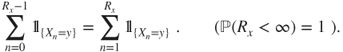
These two sums are in correspondence by a step of the chain, and we will see that an invariant measure is obtained by taking expectations.
The canonical invariant measure is above all a theoretical tool and is usually impossible to compute. It has just been used to prove that any Markov chain with a recurrent state has an invariant measure. It will be used again in the following uniqueness theorem, the proof of which is due to C. Derman, and uses a minimality result quite similar to Theorem 2.2.2.
3.2.3 Positive recurrence, invariant law criterion
Let ![]() be a Markov chain, and
be a Markov chain, and ![]() for
for ![]() in
in ![]() . A recurrent state
. A recurrent state ![]() is said to be either null recurrent or positive recurrent according to the alternative
is said to be either null recurrent or positive recurrent according to the alternative
A transition matrix or Markov chain is said to be positive recurrent if all the states are so. The following fundamental result establishes a strong link between this sample path property and an algebraic property.
3.2.3.1 Finite state space
The following simple corollary is very important in practice and can readily be proved directly.
3.2.3.2 Mean return time in a finite set
We give an extension of this result, which is quite useful for certain positive recurrence criteria.
3.2.4 Detailed examples
3.2.4.1 Nearest-neighbor walk in one dimension
The nearest-neighbor random walk on ![]() with probability
with probability ![]() of going to the right and
of going to the right and ![]() of going to the left is an irreducible Markov chain (see Section 3.1.3). The local balance equations are given by
of going to the left is an irreducible Markov chain (see Section 3.1.3). The local balance equations are given by
and have solution ![]() . The global balance equations are given by
. The global balance equations are given by
and this second-order linear recursion has characteristic polynomial
with roots ![]() and
and ![]() , possibly equal.
, possibly equal.
If ![]() , then the invariant measures are of the form
, then the invariant measures are of the form ![]() for all
for all ![]() and
and ![]() s.t.
s.t. ![]() . There is nonuniqueness of the invariant measure, and Theorem 3.2.3 yields that the random walk is transient.
. There is nonuniqueness of the invariant measure, and Theorem 3.2.3 yields that the random walk is transient.
If ![]() , then the general solution for the global balance equation is
, then the general solution for the global balance equation is ![]() , and the nonnegative solutions are of constant equal to
, and the nonnegative solutions are of constant equal to ![]() . Hence, the uniform measure is the unique invariant measure, and as it is of infinite mass there is no invariant law. The invariant law criterion (Theorem 3.2.4) yields that this chain is not positive recurrent.
. Hence, the uniform measure is the unique invariant measure, and as it is of infinite mass there is no invariant law. The invariant law criterion (Theorem 3.2.4) yields that this chain is not positive recurrent.
In Section 3.1.3, we have used the study of the unilateral hitting time to prove that for ![]() the chain is recurrent, and hence, it is null recurrent.
the chain is recurrent, and hence, it is null recurrent.
We have given examples, when ![]() in which there is nonuniqueness of the invariant measure, and when
in which there is nonuniqueness of the invariant measure, and when ![]() in which the uniqueness result in Theorem 3.2.3 requires the nonnegativity assumption.
in which the uniqueness result in Theorem 3.2.3 requires the nonnegativity assumption.
3.2.4.2 Symmetric random walk in many dimensions
For the symmetric random walk on ![]() for
for ![]() , the unique invariant measure is uniform. As it has infinite mass, there is no invariant law. The invariant law criterion (Theorem 3.2.4) yields that this chain is not positive recurrent.
, the unique invariant measure is uniform. As it has infinite mass, there is no invariant law. The invariant law criterion (Theorem 3.2.4) yields that this chain is not positive recurrent.
We have used the Potential matrix criterion in Section 3.1.3 to prove that in dimension ![]() and
and ![]() the random walk is recurrent, and hence null recurrent, whereas in dimension
the random walk is recurrent, and hence null recurrent, whereas in dimension ![]() it is transient.
it is transient.
3.2.4.3 Nearest-neighbor walk in one dimension reflected at 0
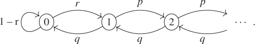
Let us consider the random walk on ![]() reflected at
reflected at ![]() , for which
, for which ![]() and
and ![]() for
for ![]() and at the boundary
and at the boundary ![]() and
and ![]() , with graph
, with graph
Two cases of particular interest are ![]() and
and ![]() .
.
The global balance equations are given by
Hence, ![]() and then
and then ![]() , and clearly the recursion then determines
, and clearly the recursion then determines ![]() for
for ![]() , so that there is uniqueness of the invariant measure.
, so that there is uniqueness of the invariant measure.
The values ![]() for
for ![]() could be determined under the general form
could be determined under the general form ![]() if
if ![]() or
or ![]() if
if ![]() , by determining
, by determining ![]() and
and ![]() using the values for
using the values for ![]() and
and ![]() , but it is much simpler to use the local balance equations.
, but it is much simpler to use the local balance equations.
The local balance equations are
and thus ![]() and
and ![]() for
for ![]() , and hence,
, and hence,
For ![]() , this is a geometric sequence.
, this is a geometric sequence.
If ![]() , then
, then ![]() and the invariant law criterion (Theorem 3.2.4) yields that the chain is positive recurrent. For
and the invariant law criterion (Theorem 3.2.4) yields that the chain is positive recurrent. For ![]() ,
,
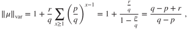
and the unique invariant law is given by ![]() . For
. For ![]() , it holds that
, it holds that
and for ![]() we obtain the geometric law
we obtain the geometric law ![]() for
for ![]() .
.
If ![]() , then this measure has infinite mass, and the chain cannot be positive recurrent. The results on the unilateral hitting time, or on the nearest-neighbor random walk on
, then this measure has infinite mass, and the chain cannot be positive recurrent. The results on the unilateral hitting time, or on the nearest-neighbor random walk on ![]() , yield that the chain is null recurrent if
, yield that the chain is null recurrent if ![]() and transient if
and transient if ![]() .
.
3.2.4.4 Ehrenfest Urn
See Section 1.4.4. The chains ![]() on
on ![]() and
and ![]() on
on ![]() are irreducible, and Corollary 3.2.7 yields that they are positive recurrent.
are irreducible, and Corollary 3.2.7 yields that they are positive recurrent.
We have seen that the invariant law of ![]() is the uniform law on
is the uniform law on ![]() , and deduced from this that the invariant law of
, and deduced from this that the invariant law of ![]() is binomial
is binomial ![]() , given by
, given by
We also can recover the invariant law of ![]() by solving the local balance equation, given by
by solving the local balance equation, given by
see (1.4.4), and hence,
Finding the invariant law ![]() reduces now to computing the normalizing constant
reduces now to computing the normalizing constant
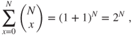
and we again find that ![]() .
.
Such a normalizing problem happens systematically, and may well be untractable, be it the computation of an infinite sum or of a huge combinatorial finite sum.
Mean time to return to vacuum
Starting at ![]() , the mean waiting time before compartment
, the mean waiting time before compartment ![]() is empty again is given by
is empty again is given by
This is absolutely enormous for ![]() of the order of the Avogadro's number. Compared to it, the duration of the universe is absolutely negligible (in an adequate timescale).
of the order of the Avogadro's number. Compared to it, the duration of the universe is absolutely negligible (in an adequate timescale).
Mean time to return to balanced state
Consider state ![]() , which is a well-balanced state. It is the mean value of
, which is a well-balanced state. It is the mean value of ![]() in equilibrium if
in equilibrium if ![]() is even, or else the nearest integer below it. According to whether
is even, or else the nearest integer below it. According to whether ![]() is even or odd,
is even or odd,
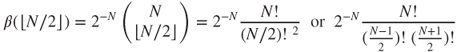
and the Stirling formula ![]() yields that
yields that
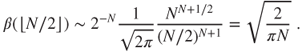
Thus
and ![]() is even small compared to the number of molecules
is even small compared to the number of molecules ![]() , the inverse of which should give the order of magnitude of the time-step.
, the inverse of which should give the order of magnitude of the time-step.
Refutation of the Refutation of statistical mechanics
This model was given by the Ehrenfest spouses as a refutation of critiques of statistical mechanics based on the fact that such a random evolution would visit all states infinitely often, even the less likely ones.
We see how important it is to obtain a wholly explicit invariant law. In particular it is important to compute the normalizing factor for a known invariant measure, or at least to derive a good approximation for it. This is a classic difficulty encountered in statistical mechanics in order to obtain useful results.
3.2.4.5 Renewal process
See Section 1.4.5. Assume that ![]() is irreducible. A necessary and sufficient condition for
is irreducible. A necessary and sufficient condition for ![]() to be recurrent is that
to be recurrent is that
and this is also the necessary and sufficient condition for the existence of an invariant measure. We have given an explicit expression for the invariant measure when it exists, and shown that then it is unique.
A necessary and sufficient condition for the existence of an invariant law ![]() is that
is that
and we have given an explicit expression for ![]() when it exists. By the invariant law criterion, this is also a necessary and sufficient condition for positive recurrence.
when it exists. By the invariant law criterion, this is also a necessary and sufficient condition for positive recurrence.
All this is actually obvious, as ![]() when
when ![]() .
.
Note that if ![]() , then the renewal process is an example of an irreducible Markov chain having no invariant measure.
, then the renewal process is an example of an irreducible Markov chain having no invariant measure.
3.2.4.6 Word search
See Section 1.4.6. The chain is irreducible on a finite state space, so that Corollary 3.2.7 of the invariant law criterion yields that it is positive recurrent. Its invariant law was computed at the end of Section 1.2.
3.2.4.7 Snake chain
See Section 1.4.6, where we proved that if ![]() has an invariant law then so does
has an invariant law then so does ![]() . The invariant law criterion yields that if
. The invariant law criterion yields that if ![]() is irreducible positive recurrent on
is irreducible positive recurrent on ![]() , then so is
, then so is ![]() on its natural state space
on its natural state space ![]() . It is clear that if
. It is clear that if ![]() is null recurrent for
is null recurrent for ![]() , then
, then ![]() cannot be positive recurrent for
cannot be positive recurrent for ![]() , and hence is null recurrent.
, and hence is null recurrent.
3.2.4.8 Product chain
See Section 1.4.7. One must be well aware that ![]() and
and ![]() may be irreducible without
may be irreducible without ![]() being so.
being so.
The decomposition in recurrent classes and the invariant law criterion yield that if for ![]() every state is positive recurrent for
every state is positive recurrent for ![]() , then there exists invariant laws
, then there exists invariant laws ![]() for
for ![]() . Then,
. Then, ![]() is an invariant law for
is an invariant law for ![]() , which is hence positive recurrent.
, which is hence positive recurrent.
If for ![]() every state is null recurrent for
every state is null recurrent for ![]() , then
, then ![]() may be either transient or null recurrent (see Exercise 3.2).
may be either transient or null recurrent (see Exercise 3.2).
3.3 Complements
This is a section giving some openings toward theoretical and practical tools for the study of Markov chains in the perspective of this chapter.
3.3.1 Hitting times and superharmonic functions
3.3.1.1 Superharmonic, subharmonic, and harmonic functions
A function ![]() on
on ![]() is said to be harmonic if
is said to be harmonic if ![]() , or equivalently if
, or equivalently if ![]() , that is, if it is an eigenvector of
, that is, if it is an eigenvector of ![]() for the eigenvalue
for the eigenvalue ![]() . A function
. A function ![]() is said to be superharmonic if
is said to be superharmonic if ![]() and to be subharmonic if
and to be subharmonic if ![]() .
.
Note that a function ![]() is subharmonic if and only if
is subharmonic if and only if ![]() is superharmonic and harmonic if and only if
is superharmonic and harmonic if and only if ![]() is both superharmonic and subharmonic.
is both superharmonic and subharmonic.
The constant functions are harmonic, and a natural question is whether these are the only harmonic functions. Theorem 2.2.2 will be very useful in this perspective, for instance, it yields that
is the least nonnegative superharmonic function, which is larger than ![]() on
on ![]() .
.
This theorem recalls Theorem 3.2.3, and we will develop in Lemma 3.3.9 and thereafter an appropriate duality to deduce one from the other. Care must be taken, as there exists transient transition matrices without any invariant measure, see the renewal process for ![]() ; others with a unique invariant measure, see the nearest-neighbor random walks reflected at
; others with a unique invariant measure, see the nearest-neighbor random walks reflected at ![]() on
on ![]() ; and others with nonunique invariant laws, see the nearest-neighbor random walks on
; and others with nonunique invariant laws, see the nearest-neighbor random walks on ![]() .
.
3.3.1.2 Supermartingale techniques
It is instructive to give two proofs of the “only if” part of Theorem 3.3.1 (the most difficult) using supermartingale concepts.
We assume that ![]() is nonnegative superharmonic and that
is nonnegative superharmonic and that ![]() is irreducible recurrent. A fundamental observation is that if
is irreducible recurrent. A fundamental observation is that if ![]() is a Markov chain and
is a Markov chain and ![]() is superharmonic, then
is superharmonic, then ![]() is a supermartingale.
is a supermartingale.
First Proof
This uses a deep result of martingale theory, the Doob convergence theorem, which yields that the nonnegative supermartingale ![]() converges, a.s. Moreover, as
converges, a.s. Moreover, as ![]() is recurrent,
is recurrent, ![]() visits infinitely often
visits infinitely often ![]() for every
for every ![]() in
in ![]() . This is only possible if
. This is only possible if ![]() is constant.
is constant.
Second Proof (J.L. Doob)
This uses more elementary results. Let ![]() and
and ![]() be in
be in ![]() , and
, and
Then, ![]() and the stopped process
and the stopped process ![]() are supermartingales, and thus
are supermartingales, and thus
and as ![]() by Lemma 3.1.3, the Fatou lemma (Lemma A.3.3) yields that
by Lemma 3.1.3, the Fatou lemma (Lemma A.3.3) yields that
Hence, ![]() is constant, as
is constant, as ![]() and
and ![]() are arbitrary.
are arbitrary.
In this and the following proofs, we have elected to use results in Markov chain theory such as Lemma 3.1.3 as much as possible but could replace them by the Doob convergence theorem to prove convergences.
3.3.2 Lyapunov functions
The main intuition behind the second proof is that the supermartingale ![]() has difficulty going uphill in the mean.
has difficulty going uphill in the mean.
This leads naturally to the notion of Lyapunov function, which is a function of which the behavior on sample paths allows to determine the behavior of the latter: go to infinity and then the chain is transient, come always back to a given finite set and then the chain is recurrent, do so quickly and then the chain is positive recurrent.
We give some examples of such results among a wide variety, in a way greatly inspired by the presentation by Robert, P. (2003).
3.3.2.1 Transience and nonpositive-recurrence criteria
A simple corollary of the “only if” part of Theorem 3.3.1 allows to get rid of a subset ![]() of the state space
of the state space ![]() in which the Markov chain behaves “poorly.”
in which the Markov chain behaves “poorly.”
It is a simple matter to adapt the proof using Theorem 2.2.2 or the second supermartingale proof for Theorem 3.3.1, and this is left as an exercise.
Note that ![]() and that we may assume that
and that we may assume that ![]() . The functions under consideration are basically upper-bounded subharmonic and nonnegative.
. The functions under consideration are basically upper-bounded subharmonic and nonnegative.
The sequel is an endeavor to replace the upper-bound assumption by integrability assumptions. Let us start with a variant of results due to J. Lamperti.
The next criterion, due to R. Tweedie, uses a submartingale and a direct computation of ![]() convergence.
convergence.
3.3.2.2 Positive recurrence criteria
Such criteria cannot be based on solid results such as Theorem 3.3.1 and are more delicate. We are back to functions that are basically nonnegative superharmonic and to supermartingales.
Theorem 3.3.5 in conjunction with Theorem 3.3.4 provides a null recurrence criterion. Under stronger assumptions, a positive recurrence criterion is obtained.