
Chapter 5
Monte Carlo methods
Monte Carlo methods based on Markov chains are often called MCMC methods, the acronym “MCMC” standing for “Markov Chain Monte Carlo.” These are often the only effective methods for the approximate computation of highly combinatorial quantities of interest and may be introduced even in situations in which the basic model is deterministic.
The corresponding research field is at the crossroads of disciplines such as statistics, stochastic processes, and computer science, as well as of various applied sciences that use it as a computation tool. It is the subject of a vast modern literature.
We are going to explain the main bases for these methods and illustrate them on some classic examples. We hope that we thus shall help the readers appreciate their adaptability and efficiency. This chapter thus provides better understanding on the practical importance of Markov chains, as well as some of the problematics they introduce.
5.1 Approximate solution of the Dirichlet problem
5.1.1 General principles
The central idea is to use Theorem 2.2.2, not any longer for computing
by solving the equation as we have done, but on the contrary to use this probabilistic representation in order to approximate the solution of the Dirichlet problem. If
then the strong law of large numbers yields a Monte Carlo method for this.
The corresponding MCMC method consists in simulating ![]() independent chains of matrix
independent chains of matrix ![]() starting at
starting at ![]() , denoted by
, denoted by ![]() for
for ![]() , each until its first exit time
, each until its first exit time ![]() from
from ![]() , and use that
, and use that
In order to obtain confidence intervals for this method, one can use for instance
- the central limit theorem, which requires information on the variance

- exponential Markov inequalities, or a large deviation principle, which requires information on the exponential moments of
 .
.
The central limit theorem or a large deviation principle actually only yield asymptotic confidence intervals.
Naturally, this requires that ![]() , and even that
, and even that ![]() as another application of the strong law of large numbers yields that the total number of time steps for
as another application of the strong law of large numbers yields that the total number of time steps for ![]() simulations is
simulations is
Hence, the obtention of exact or approximate solutions of the equations in Theorems 2.2.5 and 2.2.6 would allow to handle some essential problems, such as
- the estimation of the mean number of steps
required for each simulation,
- the establishment of confidence intervals on the duration of the simulation of one of the Markov chains and on the total duration

of the
 simulations: this can be obtained using
  and
and  and the central limit theorem, or using
  and exponential Markov inequalities if the convergence radius is greater than
  ,
, - the development of criteria for abandoning simulations, which are too long, and for compensating the bias induced by these censored data.
5.1.2 Heat equation in equilibrium
5.1.2.1 Dirichlet problem
The Dirichlet problem for the stationary heat equation on a domain ![]() of
of ![]() with boundary condition
with boundary condition ![]() is given, denoting the Laplacian by
is given, denoting the Laplacian by ![]() , by
, by
It corresponds to the physical problem of describing the temperature distribution in equilibrium of a homogeneous solid occupying ![]() , which is heated at its boundary
, which is heated at its boundary ![]() according to a temperature distribution given by
according to a temperature distribution given by ![]() . Physically,
. Physically, ![]() w.r.t. the absolute zero, and the solution is the minimal solution.
w.r.t. the absolute zero, and the solution is the minimal solution.
5.1.2.2 Discretization
Let us discretize space by a regular grid with mesh of size ![]() . A natural approximation of
. A natural approximation of ![]() is given by
is given by

Considering the transition matrix ![]() of the symmetric nearest-neighbor random walk
of the symmetric nearest-neighbor random walk ![]() on the grid, an approximation
on the grid, an approximation ![]() of
of ![]() on the grid, the set
on the grid, the set ![]() of gridpoints outside
of gridpoints outside ![]() , which are at a distance
, which are at a distance ![]() , and an appropriate approximation
, and an appropriate approximation ![]() of
of ![]() on
on ![]() , yields the discretized problem
, yields the discretized problem
The quality of the approximation of the initial problem by the discretized problem can be treated by analytic methods or by probabilistic methods using the approximation of Brownian motion by random walks. Note that if ![]() is bounded with “characteristic length”
is bounded with “characteristic length” ![]() then the number of points in
then the number of points in ![]() is of order
is of order ![]() .
.
5.1.2.3 Monte Carlo approximation
Let ![]() be the exit time of
be the exit time of ![]() from
from ![]() . Theorem 2.2.2 yields that if
. Theorem 2.2.2 yields that if ![]() is nonnegative then the least nonnegative solution of the discretized problem is given by the probabilistic representation
is nonnegative then the least nonnegative solution of the discretized problem is given by the probabilistic representation
and that if ![]() is bounded and moreover
is bounded and moreover ![]() for every
for every ![]() then
then ![]() is the unique bounded solution. For
is the unique bounded solution. For ![]() , a Monte Carlo approximation
, a Monte Carlo approximation ![]() of
of ![]() is obtained as in (5.1.1).
is obtained as in (5.1.1).
Note that ![]() as soon as
as soon as ![]() is bounded in at least one principal direction: the effective displacement along this axis will form a symmetric nearest-neighbor random walk on
is bounded in at least one principal direction: the effective displacement along this axis will form a symmetric nearest-neighbor random walk on ![]() , which always eventually reaches a unilateral boundary, as we have seen.
, which always eventually reaches a unilateral boundary, as we have seen.
When ![]() is bounded, the result (2.3.10) on the exit time from a box provides a bound on the expectation of the duration of a simulation. In particular, if
is bounded, the result (2.3.10) on the exit time from a box provides a bound on the expectation of the duration of a simulation. In particular, if ![]() has “characteristic length”
has “characteristic length” ![]() then the mean number of steps for obtaining the Monte Carlo approximation is of order
then the mean number of steps for obtaining the Monte Carlo approximation is of order
5.1.3 Heat equation out of equilibrium
5.1.3.1 Dirichlet problem
There is an initial heat distribution ![]() on
on ![]() , and for
, and for ![]() , a heat distribution
, a heat distribution ![]() is applied to
is applied to ![]() . The Monte Carlo method is well adapted to this nonequilibrium situation, in which time will be considered as a supplementary spatial dimension, and the initial condition as a boundary condition.
. The Monte Carlo method is well adapted to this nonequilibrium situation, in which time will be considered as a supplementary spatial dimension, and the initial condition as a boundary condition.
With an adequate choice of the units of time and space in terms of the thermal conductance of the medium,

5.1.3.2 Discretization
Discretizing by a spatial mesh of size ![]() and a temporal mesh of size
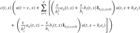
and a temporal mesh of size ![]() yields
yields
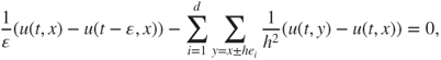
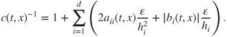
which writes ![]() for the transition matrix
for the transition matrix ![]() given by
given by
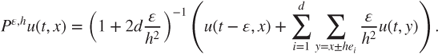
Hence, ![]() and
and ![]() should be of the same order for this diffusive phenomenon. By approximating adequately
should be of the same order for this diffusive phenomenon. By approximating adequately ![]() by
by ![]() on
on ![]() , the discretized problem writes
, the discretized problem writes

This constitutes a discretization scheme, implicit in time, for the heat equation, which is unconditionally stable: there is no need for a CFL condition. This scheme has many advantages over an explicit scheme.
The quality of the approximation of the initial problem by the discretized problem can be treated by analytic methods or by probabilistic methods using the approximation of Brownian motion by random walks.
Curse of dimensionality
The deterministic numerical solution of this scheme requires to solve a linear system at each time step. If the domain ![]() is bounded with “characteristic length”
is bounded with “characteristic length” ![]() , then
, then ![]() has cardinality of order
has cardinality of order ![]() . The deterministic methods hence become quickly untractable as
. The deterministic methods hence become quickly untractable as ![]() increases even to moderate sizes. Such difficulties are referred to by the terminology “the curse of dimensionality,” due to Bellman.
increases even to moderate sizes. Such difficulties are referred to by the terminology “the curse of dimensionality,” due to Bellman.
5.1.3.3 Monte Carlo approximation
Monte Carlo methods provide very good alternative techniques bypassing this curse. Let ![]() be the hitting time of
be the hitting time of
by the chain ![]() with matrix
with matrix ![]() . For
. For ![]() in
in ![]() , Theorem 2.2.2 yields that if
, Theorem 2.2.2 yields that if ![]() is nonnegative (resp. bounded) then the least nonnegative solution (resp. the unique bounded solution) of the above discretization scheme is given by the probabilistic representation
is nonnegative (resp. bounded) then the least nonnegative solution (resp. the unique bounded solution) of the above discretization scheme is given by the probabilistic representation

At each time step, the first coordinate of ![]() advances of
advances of ![]() with probability
with probability ![]() , and hence
, and hence ![]() where
where ![]() for
for ![]() which are i.i.d., and have geometric law given by
which are i.i.d., and have geometric law given by ![]() for
for ![]() . Simple computations show that
. Simple computations show that ![]() is finite, a.s., has some finite exponential moments, and
is finite, a.s., has some finite exponential moments, and

so that we have bounds linear in the dimension ![]() for the expectation and the standard deviation.
for the expectation and the standard deviation.
Then, ![]() can be approximated using the Monte Carlo method by
can be approximated using the Monte Carlo method by ![]() given in (5.1.1). The central limit theorem yields that the precision is of order
given in (5.1.1). The central limit theorem yields that the precision is of order ![]() with a constant that depends on the variance and hence very reasonably on the dimension
with a constant that depends on the variance and hence very reasonably on the dimension ![]() .
.
This is a huge advantage of Monte Carlo methods over deterministic methods, which suffer of the curse of dimensionally and of which the complexity increases much faster with the dimension.
5.1.4 Parabolic partial differential equations
5.1.4.1 Dirichlet problem
More general parabolic problems may be considered. Let a time-dependent elliptic operator acting on ![]() in
in ![]() be given by
be given by
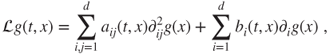
where the matrix ![]() is symmetric nonnegative. Consider the Dirichlet problem
is symmetric nonnegative. Consider the Dirichlet problem

5.1.4.2 Discretization: diagonal case
Let us first assume that ![]() is diagonal. It is always possible to find an orthonormal basis in which is locally the case, corresponding to the principal axes of
is diagonal. It is always possible to find an orthonormal basis in which is locally the case, corresponding to the principal axes of ![]() , and it is a good idea to find them if
, and it is a good idea to find them if ![]() is constant. By discretizing the
is constant. By discretizing the ![]() th coordinate by a step of
th coordinate by a step of ![]() and time by a step of
and time by a step of ![]() ,
,

This writes ![]() for the transition matrix
for the transition matrix ![]() equal to
equal to
in which the normalizing constant is given by
This is again a discretization scheme for the PDE, which is implicit in time and unconditionally stable. Then, ![]() should be of the same order than
should be of the same order than ![]() if
if ![]() and of same order as
and of same order as ![]() if
if ![]() . The relative choices for the
. The relative choices for the ![]() should be influenced by the sizes of the
should be influenced by the sizes of the ![]() or the
or the ![]() , and in particular if
, and in particular if ![]() is constant in
is constant in ![]() , then a good choice would be
, then a good choice would be ![]() if
if ![]() and
and ![]() if
if ![]() .
.
5.1.4.3 Monte Carlo approximation
The matrix ![]() is a transition matrix, and the previous probabilistic representations and Monte Carlo methods are readily generalized to this situation.
is a transition matrix, and the previous probabilistic representations and Monte Carlo methods are readily generalized to this situation.
5.1.4.4 Discretization: nondiagonal case
In general, a natural discretization of the Dirichlet problem is given by
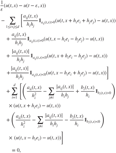
which features “diagonal” jumps, and thus extended ![]() and
and ![]() w.r.t. the previous situation.
w.r.t. the previous situation.
5.1.4.5 Monte Carlo approximation
In order to have an interpretation in terms of a transition matrix, it is necessary and sufficient that

which is not always true when ![]() , as can be seen with the matrix in which all terms are
, as can be seen with the matrix in which all terms are ![]() . It this holds for all
. It this holds for all ![]() , then the previous probabilistic representations and Monte Carlo methods can easily be extended to this situation. Else other methods will be used, which do not involve a spatial grid discretization as this causes a strong anisotropy.
, then the previous probabilistic representations and Monte Carlo methods can easily be extended to this situation. Else other methods will be used, which do not involve a spatial grid discretization as this causes a strong anisotropy.
5.2 Invariant law simulation
In this section, we mostly assume that ![]() is finite and set
is finite and set ![]() .
.
5.2.1 Monte Carlo methods and ergodic theorems
Let ![]() be a state space, and
be a state space, and ![]() a probability measure on
a probability measure on ![]() , which can be interpreted as the invariant law for an irreducible transition matrix
, which can be interpreted as the invariant law for an irreducible transition matrix ![]() . Finding an explicit expression for
. Finding an explicit expression for ![]() may raise the following difficulties.
may raise the following difficulties.
- The invariant measure
 is a nonnegative nonzero solution of the linear system
  . This develops into a system of
  equations for
  unknowns, usually highly coupled and as such difficult to solve, see the global balance equations (3.2.4). If
  is reversible, then the local balance equations (3.2.5) can be used, yielding for
  the semiexplicit expression in Lemma 3.3.8.
 - The invariant law
 has total mass
  , and thus the following normalization problem arises. Once an invariant law
  is obtained, then
  must be computed in order to make
  explicit. In general, such a summation is an NP-complete problem in terms of
  .
.
These difficulties are elegantly bypassed by Monte Carlo approximation methods. These replace the resolution of an equation, which implicitly defines an invariant measure, and the normalization of the solution, by the simulation of a Markov chain, which is explicitly given by its transition matrix.
5.2.1.1 Pointwise ergodic theorem
Assume that a real function ![]() on
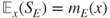
on ![]() is given and that the mean of
is given and that the mean of ![]() w.r.t.
w.r.t. ![]() is sought. We then are interested in
is sought. We then are interested in
Even if ![]() were explicitly known, such a summation is again, in general, an NP-complete problem. Recall that
were explicitly known, such a summation is again, in general, an NP-complete problem. Recall that ![]() is usually at best known only up to a normalizing constant, that is, as an invariant measure
is usually at best known only up to a normalizing constant, that is, as an invariant measure ![]() .
.
If a term ![]() of
of ![]() or the probability
or the probability ![]() of some subset of
of some subset of ![]() is sought, then this corresponds to taking
is sought, then this corresponds to taking ![]() or
or ![]() . Note that if an invariant law
. Note that if an invariant law ![]() is known and a term
is known and a term ![]() has been computed, then
has been computed, then
The pointwise ergodic theorem (Theorem 4.1.1) yields a Monte Carlo method for approximating ![]() . Indeed, if
. Indeed, if ![]() is a Markov chain with matrix
is a Markov chain with matrix ![]() and arbitrary initial condition, then
and arbitrary initial condition, then

The Markov chain central limit theorem (Theorem 4.1.5) yields confidence intervals for this convergence.
5.2.1.2 Kolmogorov's ergodic theorem
Some situations require to simulate random variables of law ![]() , for instance in view of integrating them in simulations of more complex systems. Even if
, for instance in view of integrating them in simulations of more complex systems. Even if ![]() were explicitly known, this is usually a very difficult task if
were explicitly known, this is usually a very difficult task if ![]() is large; moreover,
is large; moreover, ![]() is usually at best known only up to a normalizing constant.
is usually at best known only up to a normalizing constant.
If ![]() is aperiodic, then the Kolmogorov ergodic theorem yields a Monte Carlo method for obtaining samples drawn from an approximation of
is aperiodic, then the Kolmogorov ergodic theorem yields a Monte Carlo method for obtaining samples drawn from an approximation of ![]() . Indeed, if
. Indeed, if ![]() is a Markov chain with matrix
is a Markov chain with matrix ![]() and arbitrary initial condition, then
and arbitrary initial condition, then
Exponential convergence bounds are given by Theorem 1.3.4, in terms of the Doeblin condition, which is satisfied, but usually the bounds are very poor. Much better exponential bounds are given in various results and developments around the Dirichlet forms, spectral gap estimations, and Poincaré inequalities, which have been introduced in Section 4.3.
5.2.2 Metropolis algorithm, Gibbs law, and simulated annealing
5.2.2.1 Metropolis algorithm
Let ![]() be a law of interest, determined at least up to a normalizing constant. It may be given for instance by statistical mechanics considerations. The first step is to interpret
be a law of interest, determined at least up to a normalizing constant. It may be given for instance by statistical mechanics considerations. The first step is to interpret ![]() as the reversible law (and thus the invariant law) of an explicit transition matrix
as the reversible law (and thus the invariant law) of an explicit transition matrix ![]() .
.
Let ![]() be an irreducible transition matrix
be an irreducible transition matrix ![]() on
on ![]() , called the selection matrix, s.t.
, called the selection matrix, s.t. ![]() for
for ![]() in
in ![]() , and a function
, and a function
for instance ![]() or
or ![]() . Let
. Let
which depends on ![]() only up to a normalizing constant. Let
only up to a normalizing constant. Let ![]() be defined by
be defined by
with ![]() if
if ![]() and
and ![]() .
.
It is a simple matter to check that ![]() is an irreducible transition matrix, which is reversible w.r.t.
is an irreducible transition matrix, which is reversible w.r.t. ![]() , and that
, and that ![]() is aperiodic if
is aperiodic if ![]() is aperiodic or if
is aperiodic or if ![]() . Hence, the above-mentioned Monte Carlo methods for approximating quantities related to
. Hence, the above-mentioned Monte Carlo methods for approximating quantities related to ![]() can be implemented using
can be implemented using ![]() .
.
The Metropolis algorithm is a method for sequentially drawing a sample ![]() of a Markov chain
of a Markov chain ![]() of transition matrix
of transition matrix ![]() , using directly
, using directly ![]() and
and ![]() :
:
- Step
 (initialization): draw
  according to the arbitrary initial law.
 - Step
 (from
(from  to
to  ): draw
  according to the law
  :
:
- with probability
 set
set 
- else set
 .
.
- with probability
This is an acceptance–rejection method: the choice of a candidate for a new state ![]() is made according to
is made according to ![]() and is accepted with probability
and is accepted with probability ![]() and else rejected. The actual evolution is thus made in accordance with
and else rejected. The actual evolution is thus made in accordance with ![]() , which has invariant law
, which has invariant law ![]() , instead of
, instead of ![]() .
.
A classic case uses ![]() given by
given by ![]() . Then,
. Then, ![]() is accepted systematically if
is accepted systematically if
and else with probability
5.2.2.2 Gibbs laws and Ising model
Let ![]() be a function and
be a function and ![]() a real number. The Gibbs law with energy function
a real number. The Gibbs law with energy function ![]() and temperature
and temperature ![]() is given by
is given by

This law characterizes the thermodynamical equilibrium of a system in which an energy ![]() corresponds to each configuration
corresponds to each configuration ![]() . More precisely, it is well known that among all laws
. More precisely, it is well known that among all laws ![]() for which the mean energy
for which the mean energy ![]() has a given value
has a given value ![]() , the physical entropy
, the physical entropy
is maximal for a Gibbs law ![]() for a well-defined
for a well-defined ![]() .
.
Owing to the normalizing constant, ![]() does not change if a constant is added to
does not change if a constant is added to ![]() , and hence
, and hence
the uniform law on the set of minima of ![]() .
.
Ising model
A classic example is given by the Ising model. This is a magnetic model, in which ![]() and the energy of configuration
and the energy of configuration ![]() is given by
is given by

in which the matrix ![]() can be taken symmetric and with a null diagonal, and
can be taken symmetric and with a null diagonal, and ![]() and
and ![]() are the two possible orientations if a magnetic element at site
are the two possible orientations if a magnetic element at site ![]() . The term
. The term ![]() quantifies the interaction between the two sites
quantifies the interaction between the two sites ![]() , for instance
, for instance ![]() for a ferromagnetic interaction in which configurations
for a ferromagnetic interaction in which configurations ![]() are favored. The term
are favored. The term ![]() corresponds to the effect of an external magnetic field on site
corresponds to the effect of an external magnetic field on site ![]() .
.
The state space ![]() has cardinal
has cardinal ![]() , so that the computation or even estimation of the normalizing constant
, so that the computation or even estimation of the normalizing constant ![]() , called the partition function, is very difficult as soon as
, called the partition function, is very difficult as soon as ![]() is not quite small.
is not quite small.
Simulation
The simulation by the Metropolis algorithm is straightforward. Let ![]() be an irreducible matrix on
be an irreducible matrix on ![]() , for instance corresponding to choosing uniformly
, for instance corresponding to choosing uniformly ![]() in
in ![]() and changing
and changing ![]() into
into ![]() . The algorithm proceeds as follows:
. The algorithm proceeds as follows:
- Step
 (initialization): draw
  according to the arbitrary initial law.
 - Step
 (from
(from  to
to  ): draw
  according to the law
  :
:
- set
 with probability

- else set
 .
.
- set
If moreover ![]() and
and ![]() , then
, then ![]() is accepted systematically if
is accepted systematically if
and else with probability
5.2.2.3 Global optimization and simulated annealing
A deterministic algorithm for the minimization of ![]() would only accept states that actually decrease the energy function
would only accept states that actually decrease the energy function ![]() . They allow to find a local minimum for
. They allow to find a local minimum for ![]() , which may be far from the global minimum.
, which may be far from the global minimum.
The Metropolis algorithms also accepts certain states that increase the energy, with a probability, which decreases sharply if the energy increase is large of the temperature ![]() is low. This allows it to escape from local minima and explore the state space, and its instantaneous laws converge to the Gibbs
is low. This allows it to escape from local minima and explore the state space, and its instantaneous laws converge to the Gibbs ![]() , which distributes its mass mainly close to the global minima. We recall (5.2.2): the limit as
, which distributes its mass mainly close to the global minima. We recall (5.2.2): the limit as ![]() goes to zero of
goes to zero of ![]() is the uniform law on the minima of
is the uniform law on the minima of ![]() .
.
Let ![]() be a sequence of temperatures, and
be a sequence of temperatures, and ![]() the inhomogeneous Markov chain for which
the inhomogeneous Markov chain for which
where the transition matrix ![]() has invariant law
has invariant law ![]() , for instance corresponds to the Metropolis algorithm of energy function
, for instance corresponds to the Metropolis algorithm of energy function ![]() and temperature
and temperature ![]() .
.
A natural question is whether it is possible to choose ![]() decreasing to
decreasing to ![]() in such a way that the law of
in such a way that the law of ![]() converges to the uniform law on the minima of
converges to the uniform law on the minima of ![]() . This will yield a stochastic optimization algorithm for
. This will yield a stochastic optimization algorithm for ![]() , in which the chain
, in which the chain ![]() will be simulated for a sufficient length of time (also to be estimated), and then the instantaneous values should converge to a global minimum of
will be simulated for a sufficient length of time (also to be estimated), and then the instantaneous values should converge to a global minimum of ![]() .
.
From a physical viewpoint, this is similar to annealing techniques in metallurgy, in which an alloy is heated and then its temperature let decrease sufficiently slowly that the final state is close to a energy minimum. In quenched techniques, on the contrary, the alloy is plunged into a cold bath in order to obtain a desirable state close to a local minimum.
Clearly, the temperature should be let decrease sufficiently slowly. The resulting theoretic results, see for example Duflo, M. (1996, Section 6.4, p. 264), are for logarithmic temperature decrease, for instance of the form ![]() or
or ![]()
![]() for large enough
for large enough ![]() .
.
This is much too slow in practice, and temperatures are let decrease much faster than that in actual algorithms. These nevertheless provide good results, in particular high-quality suboptimal values in combinatorial optimization problems.
5.2.3 Exact simulation and backward recursion
5.2.3.1 Identities in law and backward recursion
The random recursion in Theorem 1.2.3, given by
where ![]() is a sequence of i.i.d. random functions from
is a sequence of i.i.d. random functions from ![]() to
to ![]() , which is independent of the r.v.
, which is independent of the r.v. ![]() of
of ![]() , allows to construct a Markov chain
, allows to construct a Markov chain ![]() on
on ![]() with matrix
with matrix ![]() of generic term
of generic term ![]() . In particular,
. In particular, ![]() has law
has law ![]() .
.
As the ![]() are i.i.d., the random functions
are i.i.d., the random functions ![]() and
and ![]() have same law, and if
have same law, and if ![]() has law
has law ![]() and is independent of
and is independent of ![]() then
then
has also law ![]() for
for ![]() , as
, as ![]() .
.
Far past start interpretation
A possible description of ![]() is as follows. If
is as follows. If ![]() is interpreted as a draw taking the state at time
is interpreted as a draw taking the state at time ![]() to time
to time ![]() of
of ![]() , then
, then ![]() can be seen as the instantaneous value at time
can be seen as the instantaneous value at time ![]() of a Markov chain of matrix
of a Markov chain of matrix ![]() started in the past at time
started in the past at time ![]() at
at ![]() . Letting
. Letting ![]() go to infinity then corresponds to letting the initial instant tend to
go to infinity then corresponds to letting the initial instant tend to ![]() , the randomness at the different following instants remaining fixed.
, the randomness at the different following instants remaining fixed.
5.2.3.2 Coalescence and invariant law
On the event in which the random function ![]() is constant on
is constant on ![]() , for any
, for any ![]() , it holds that
, it holds that
Let ![]() for
for ![]() , and their first coalescence time
, and their first coalescence time
This is a stopping time, after which all ![]() are constant and equal. On
are constant and equal. On ![]() let
let ![]() be defined by the constant value taken by
be defined by the constant value taken by ![]() , so that
, so that ![]() for all
for all ![]() and
and ![]() . If
. If ![]() , then for any initial r.v.
, then for any initial r.v. ![]() , it holds that
, it holds that
5.2.3.3 Propp and Wilson algorithm
The Propp and Wilson algorithm uses this for the exact simulation of draws from the invariant law ![]() of
of ![]() , using the random functions
, using the random functions ![]() . The naive idea is the following.
. The naive idea is the following.
- Start with
 being the identical mapping on
  ,
, - for
 : draw
  and compute
 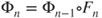 , that is,
  , and then test for coalescence:
- if
 is constant, then the algorithm terminates issuing this constant value,
 - else increment
 by
by  and continue.
- if
If the law of the ![]() is s.t.
is s.t. ![]() , then the algorithm terminates after a random number of iterations and issues a draw from
, then the algorithm terminates after a random number of iterations and issues a draw from ![]() .
.
5.2.3.4 Criteria on the coalescence time
It is important to obtain verifiable criteria for having ![]() and good estimates on
and good estimates on ![]() .
.
One criteria is to choose the law of ![]() so that there exists
so that there exists ![]() s.t.
s.t.
Then ![]() , where the
, where the ![]() are i.i.d. with geometric law
are i.i.d. with geometric law ![]() for
for ![]() . This implies that
. This implies that ![]() and
and ![]() and yields exponential bounds on the duration of the simulation.
and yields exponential bounds on the duration of the simulation.
If ![]() satisfies the Doeblin condition in Theorem 1.3.4 for
satisfies the Doeblin condition in Theorem 1.3.4 for ![]() and
and ![]() and a law
and a law ![]() , then we may consider independent r.v.
, then we may consider independent r.v. ![]() of law
of law ![]() , random functions
, random functions ![]() from
from ![]() to
to ![]() satisfying
satisfying
which may be constructed as in Section 1.2.3, and r.v. ![]() s.t.
s.t. ![]() and
and ![]() . Then, for
. Then, for ![]() ,
,
define i.i.d. random functions s.t. ![]() , for which
, for which ![]() has geometric law
has geometric law ![]() for
for ![]() .
.
Note that the algorithm can be applied to some well-chosen power ![]() of
of ![]() , which has same invariant law
, which has same invariant law ![]() and is more likely to satisfy one of the above-mentioned criteria.
and is more likely to satisfy one of the above-mentioned criteria.
5.2.3.5 Monotone systems
An important problem with the algorithm is that in order to check for coalescence it is in general necessary to simulate the ![]() for all
for all ![]() in
in ![]() , which is untractable.
, which is untractable.
Some systems are monotone, in the sense that there exists a partial ordering on ![]() denoted by
denoted by ![]() s.t. one can choose random mappings
s.t. one can choose random mappings ![]() for the random recursion satisfying, a.s.,
for the random recursion satisfying, a.s.,
If there exist a least element ![]() and a greatest
and a greatest ![]() in
in ![]() , hence s.t.
, hence s.t.
then clearly ![]() , and in order to check for coalescence, it is enough to simulate
, and in order to check for coalescence, it is enough to simulate ![]() and
and ![]() .
.
Many queuing models are of this kind, for instance the queue with capacity ![]() given by
given by
is monotone, with ![]() and
and ![]() .
.
Ising model
Another interesting example is given by the ferromagnetic Ising model, in which adjacent spins tend to have the same orientations ![]() or
or ![]() . The natural partial order is that
. The natural partial order is that ![]() if and only if
if and only if ![]() for all sites
for all sites ![]() . The least state
. The least state ![]() is the configuration constituted of all
is the configuration constituted of all ![]() , and the greatest state
, and the greatest state ![]() the configuration constituted of all
the configuration constituted of all ![]() . Many natural dynamics preserve the partial order, for instance the Metropolis algorithm we have described earlier. This is the scope of the original study in Propp, J.G. and Wilson, D.B. (1996).
. Many natural dynamics preserve the partial order, for instance the Metropolis algorithm we have described earlier. This is the scope of the original study in Propp, J.G. and Wilson, D.B. (1996).