
2.3.1.3 Generating function
Theorem 2.2.5 yields that for every ![]() the functions
the functions ![]() and
and ![]() and
and ![]() satisfy
satisfy
with boundary conditions ![]() and
and ![]() ,
, ![]() and
and ![]() , and
, and ![]() , respectively. The characteristic polynomial for this second-order linear recursion is
, respectively. The characteristic polynomial for this second-order linear recursion is
We avoid treating separately the cases ![]() and
and ![]() by considering first the case
by considering first the case ![]() , for which
, for which ![]() . Then, there are two distinct roots
. Then, there are two distinct roots
the general solution is of the form ![]() , and hence
, and hence

Using ![]() and
and
the expressions for ![]() and
and ![]() and
and ![]() can be easily recovered, which is left as an exercise.
can be easily recovered, which is left as an exercise.
Explicit joint law
A Taylor expansion yields the joint law of ![]() and of the result of the game (ruin
and of the result of the game (ruin ![]() , win if
, win if ![]() ), and hence the law of
), and hence the law of ![]() . For
. For ![]() ,
,

which yields expressions for ![]() and
and ![]() as rational functions of explicit polynomials, from which (Feller, W. (1968), XIV.5) derives the formula
as rational functions of explicit polynomials, from which (Feller, W. (1968), XIV.5) derives the formula
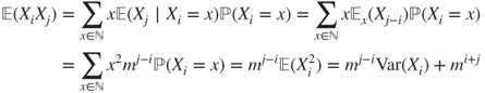
Moments
Expectations, variances, and higher moments of ![]() and
and ![]() and
and ![]() can be derived by appropriate Taylor expansions at the point
can be derived by appropriate Taylor expansions at the point ![]() for
for ![]() and
and ![]() and
and ![]() . Computations are tedious by hand but can be performed quickly by appropriate software.
. Computations are tedious by hand but can be performed quickly by appropriate software.
2.3.2 Unilateral hitting time for a random walk
Consider a compulsive Gambler A, which gambles as long as he is not ruined, starting from an initial fortune ![]() . This corresponds to taking
. This corresponds to taking ![]() and
and ![]() above. Now, the state space for
above. Now, the state space for ![]() is
is ![]() , and
, and
The game duration is ![]() , and we set
, and we set ![]() and
and ![]() . Proposition 2.2.4 does no longer apply.
. Proposition 2.2.4 does no longer apply.
2.3.2.1 Probability and mean duration for ruin
Taking limits
By monotone convergence (Theorem A.3.2),
- If
 (game biased against the gambler), then
  and
and  , and Gambler A is ruined in finite time at “speed”
  .
. - If
 (fair game), then
  and
and  , and Gambler A is eventually ruined, but the mean duration for that is infinite.
 - If
 (game biased toward the gambler), then
  and
and  and hence
  , and Gambler A is eventually ruined with probability
  , and if he does so it happens at “speed”
  . Obviously
  .
.
A global expression for this is
Direct computation
We seek the least nonnegative solutions for the equations satisfying ![]() and
and ![]() , by considering notably the behavior at infinity.
, by considering notably the behavior at infinity.
- If
 then
then  and
and  for
for  , and hence
  and
and  .
. - If
 then
then  and
and  for
for  , and hence
  and
and  for
for  .
. - If
 then
then  and
and  for
for  , and hence
 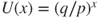 and
and  .
.
Note that if ![]() then the trivial infinite solution of the equations in Theorem 2.2.6 must be accepted, as no other solution is nonnegative. It would have been likewise if we had tried to compute thus
then the trivial infinite solution of the equations in Theorem 2.2.6 must be accepted, as no other solution is nonnegative. It would have been likewise if we had tried to compute thus ![]() for
for ![]() .
.
Fair game and debt
If ![]() then
then ![]() for a sequence
for a sequence ![]() of i.i.d. r.v. such that
of i.i.d. r.v. such that ![]() . Assuming
. Assuming ![]() ,
,
and hence ![]() , despite the fact that
, despite the fact that ![]() yields that
yields that ![]() , a.s. By dominated convergence (Theorem A.3.5), this implies that
, a.s. By dominated convergence (Theorem A.3.5), this implies that ![]() .
.
Point of view of Gambler B
The situation seems more reasonable (but less realistic) from the perspective of Gambler B, who ardently desires to gain a sum ![]() and has infinite credit and a compliant adversary. Depending on his probability
and has infinite credit and a compliant adversary. Depending on his probability ![]() of winning at each toss, his eventual win probability and expected time to win are
of winning at each toss, his eventual win probability and expected time to win are
- If
 then he wins, a.s., after a mean duration of
  .
. - If
 then he wins, a.s., but the expected time it takes is infinite, and the expectation of his maximal debt toward Gambler A is infinite.
 - If
 (as in a casino) then his probability of winning is
  , and if he attains his goal then the expected time for this is
  (else he losses an unbounded quantity of money).
2.3.2.2 Using the generating function
Let ![]() . Theorem 2.2.5 yields that for
. Theorem 2.2.5 yields that for ![]() the equation satisfied by
the equation satisfied by ![]() is the extension of (2.3.8) for
is the extension of (2.3.8) for ![]() with boundary condition
with boundary condition ![]() .
.
If ![]() then
then ![]() and the general solution is given after (2.3.9). The minimality result in Theorem 2.2.5 and the fact that
and the general solution is given after (2.3.9). The minimality result in Theorem 2.2.5 and the fact that
yield that

Expectation and variance
As ![]() and
and ![]() , it holds that
, it holds that

Classic Taylor expansions yield that, at a precision of order ![]() ,
,
and, using ![]() ,
,
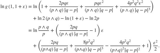
Using ![]() and by identification, see (A.1.1), this yields that
and by identification, see (A.1.1), this yields that
- if
 then
then  and
and 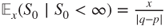 and moreover
 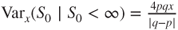 ,
, - if
 then
then  and
and  .
.
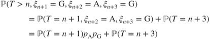
Law of game duration
The classic Taylor expansion
using the generalized binomial coefficient defined by
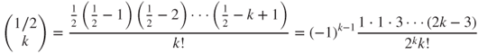
yields that
By identification, for ![]() , it holds that
, it holds that ![]() and
and
2.3.2.3 Use of the strong Markov property
The fact that
yields that the law of ![]() given that
given that ![]() is the law of the sum of
is the law of the sum of ![]() independent r.v. with same law as
independent r.v. with same law as ![]() given that
given that ![]() and implies that
and implies that
It is actually a consequence of the strong Markov property: in order for Gambler A to loose ![]() units, he must first loose
units, he must first loose ![]() unit and then he starts independently of the past from a fortune of
unit and then he starts independently of the past from a fortune of ![]() units; a simple recursion and the spatial homogeneity of a random walk conclude this. A precise formulation is left as an exercise.
units; a simple recursion and the spatial homogeneity of a random walk conclude this. A precise formulation is left as an exercise.
2.3.3 Exit time from a box
Extensions of such results to multidimensional random walks are delicate, as the linear equations are much more involved and seldom have explicit solutions. Some guesswork easily allows to find a solution in the following example.
Let ![]() be the symmetric nearest-neighbor random walk on
be the symmetric nearest-neighbor random walk on ![]() and
and ![]() be in
be in ![]() for
for ![]() . Consider
. Consider ![]() and
and ![]() , with
, with
Theorem 2.2.6 yields that the function ![]() satisfies the affine equation with boundary condition
satisfies the affine equation with boundary condition
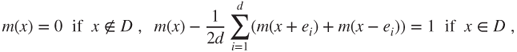
and, considering gambler's ruin, we obtain that

Notably, if ![]() and
and ![]() for
for ![]() then
then ![]() is quadratic in
is quadratic in ![]() and linear in the dimension
and linear in the dimension ![]() .
.
2.3.4 Branching process
See Section 1.4.3. We assume that
that is, that the mean number of offspring of an individual is finite, as well as ![]() and
and ![]() to avoid trivial situations. A quantity of interest is the extinction time
to avoid trivial situations. A quantity of interest is the extinction time
An essential fact is that if ![]() then
then ![]() can be obtained by the sum of the
can be obtained by the sum of the ![]() chains given by the descendants of each of the initial individuals and that these chains are independent and have same law as
chains given by the descendants of each of the initial individuals and that these chains are independent and have same law as ![]() given that
given that ![]() . In particular, we study the case when
. In particular, we study the case when ![]() , the others being deduced easily. This property can be generalized to appropriate subpopulations and is called the branching property.
, the others being deduced easily. This property can be generalized to appropriate subpopulations and is called the branching property.
Notably, if ![]() then
then ![]() for
for ![]() . This, and the “one step forward” method, yields that
. This, and the “one step forward” method, yields that
which is the recursion in Section 1.4.3, obtained there by a different method.
2.3.4.1 Probability and rate of extinction
By monotone limit (Lemma A.3.1),
Moreover, ![]() , and the recursion (2.3.11) yields that
, and the recursion (2.3.11) yields that
This recursion can also be obtained directly by the “one step forward” method: the branching property yields that ![]() , and thus
, and thus
Thus, ![]() solves the recursion
solves the recursion ![]() started at
started at ![]() , and this nondecreasing sequence converges to
, and this nondecreasing sequence converges to ![]() . As
. As ![]() is continuous on
is continuous on ![]() , the limit is the least fixed point
, the limit is the least fixed point ![]() of
of ![]() on
on ![]() . Thus, the extinction probability is
. Thus, the extinction probability is
Graphical study
The facts that ![]() and
and ![]() are continuous increasing on
are continuous increasing on ![]() , and
, and ![]() and
and ![]() and
and ![]() , allow to place the graph of
, allow to place the graph of ![]() with respect to the diagonal.
with respect to the diagonal.
- If
 then the only fixed point for
  is
is  , hence the extinction probability is
  , and the population goes extinct, a.s.
 - If
 then there exists a unique fixed point
  other than
  , and
, and  as
as  , hence the extinction probability is
  .
.
See Figure 2.3.
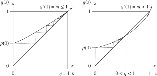
Figure 2.3 Graphical study of  with
with  . (Left)
  , and the sequence converges to
  . (Right)
  , and the sequence converges to
  , the unique fixed point of
  other than
  .
.
Moreover, the strict convexity implies that
which yields some convergence rate results.
- If
 then
then  for
for  and
and  .
.
Indeed, then
 can be written as
  for
for  , and by iteration
  and hence
  .
. - If
 then
then  for every
  .
.
Indeed,
 and thus
  , which implies the result as
  .
. - If
 then
then  for
for  , and
, and  .
.
Indeed,
 for
for  , and it is a simple matter to prove that
  (Figure 2.3).
Critical case
The case ![]() is called the critical case and is the most delicate to study. Assume that the number of offspring of a single individual has a variance or equivalently that
is called the critical case and is the most delicate to study. Assume that the number of offspring of a single individual has a variance or equivalently that ![]() or that
or that ![]() . Then
. Then ![]() , and the population goes extinct, a.s., but has an infinite mean life time.
, and the population goes extinct, a.s., but has an infinite mean life time.
Indeed, ![]() implies for
implies for ![]() that
that
and as ![]() then
then ![]() with
with
and hence ![]() .
.
2.3.4.2 Mean population size
As ![]() , an order
, an order ![]() Taylor expansion yields that
Taylor expansion yields that
and by identification ![]() and hence
and hence
This can also be directly obtained by the “one step forward” method:
A few results follow from this.
- If
 then the population mean size decreases exponentially.
 - If
 (critical case) then
  for all
  , and
, and  for a (random) large enough
  , a.s., and by dominated convergence (Theorem A.3.5)
  . Hence, the population goes extinct, a.s., but its mean size remains constant, and the expectation of its maximal size is infinite.
 - If
 then the mean size increases exponentially.
2.3.4.3 Variances and covariances
We assume ![]() . Let
. Let
denote the variance of the number of offspring of an individual, and ![]() the variance of
the variance of ![]() . As
. As ![]() , using (A.1.1), at a precision of order
, using (A.1.1), at a precision of order ![]() ,
,
and by identification
Thus, ![]() and
and
Setting ![]() , we obtain that
, we obtain that ![]() and
and
and hence
For ![]() , simple arguments yield that
, simple arguments yield that
and the covariance and correlation of ![]() and
and ![]() are given by
are given by

and more precisely
2.3.5 Word search
See Section 1.4.6. The quantity of interest is
The state space is finite and the chain irreducible, hence ![]() by Proposition 2.2.4. The expected value
by Proposition 2.2.4. The expected value ![]() and of the generating function
and of the generating function ![]() can easily be derived by solving the equations yielded by the “one step forward” method, but we leave that as an exercise.
can easily be derived by solving the equations yielded by the “one step forward” method, but we leave that as an exercise.
We prefer to describe a more direct method, which is specific to this situation. It explores some possibilities of evolution in the near future, with horizon the word length. The word GAG is constituted of three letters. As ![]() is in
is in ![]() and the sequence
and the sequence ![]() is i.i.d., for
is i.i.d., for ![]() , it holds that
, it holds that
and, considering the overlaps within the word GAG and ![]()
and hence
Expectation
As ![]() and
and ![]() , it follows that
, it follows that
Generating function
Moreover, Lemma A.1.3 yields that ![]() for
for ![]() , and (2.3.12) and
, and (2.3.12) and ![]() yield that
yield that
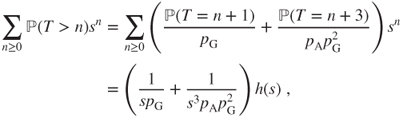
so that eventually
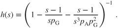
As ![]() , this yields
, this yields ![]() again. Moreover, at a precision of order
again. Moreover, at a precision of order ![]() ,
,

and (A.1.1) yields that
Exercises
2.1 Stopping times Let ![]() be a Markov chain on
be a Markov chain on ![]() , and
, and ![]() . Prove that the following random variables are stopping times.
. Prove that the following random variables are stopping times.
2.2 Operations on stopping times Let ![]() and
and ![]() be two stopping times.
be two stopping times.
- (a) Prove that
 and
and  and
and  (with value
  if
if  ) are stopping times.
 - (b) Prove that if
 then
then  , then more generally that
  .
. - (c) Prove that if
 then
then  and
and  . Deduce from this that
  , the least
  -field containing
  .
.
2.3 Induced chain, 1 Let ![]() be a Markov chain on
be a Markov chain on ![]() with matrix
with matrix ![]() , having no absorbing state. Let
, having no absorbing state. Let ![]() be defined by
be defined by ![]() and
and ![]() and iteratively
and iteratively
Let ![]() denotes the filtration generated by
denotes the filtration generated by ![]() , and
, and ![]() the one for
the one for ![]() : the events in
: the events in ![]() are of the form
are of the form ![]() , and those in
, and those in ![]() of the form
of the form ![]() . Let the matrix
. Let the matrix ![]() and for
and for ![]() , the geometric law
, the geometric law ![]() on
on ![]() be defined by
be defined by
- (a) Prove that
 is a transition matrix and that
  is irreducible if and only if
  is irreducible.
 - (b) Prove that the
 are stopping times and that
  .
. - (c) Prove that
 is a Markov chain with transition matrix given by

Prove that
 is a Markov chain with matrix
  . Prove that
- (d) Prove that if
 is a stopping time for
  , that is, for
  , then
  is a stopping time for
  , that is, for
  .
.
2.4 Doeblin coupling Let ![]() be a Markov chain on
be a Markov chain on ![]() with matrix
with matrix ![]() satisfying
satisfying
and
Let ![]() be a transition matrix on
be a transition matrix on ![]() such that there exists
such that there exists ![]() and a probability measure
and a probability measure ![]() such that
such that ![]() for all
for all ![]() ; this is the Doeblin condition of Theorem 1.3.4 for
; this is the Doeblin condition of Theorem 1.3.4 for ![]() .
.
- (a) Prove that
 is a stopping time.
 - (b) Prove that
 has same law as
  . Deduce from this, for instance using (1.2.2), that

- (c) Prove that we define transition matrices
 on
on  and
and  on
on  by
by

and that
 .
. - (d) Prove that
 .
. - (e) Prove that
 and
and  are both Markov chains with matrix
  .
. - (f) Conclude that

by using the fact that there exists r.v.
 and
and  with laws
  and
and  such that
  (see Lemma A.2.2).
2.5 The space station, see Exercise 1.1 The astronaut starts from module ![]() .
.
- (a) What is his probability of reaching module
 before visiting the central module (module
  )?
)? - (b) What is his probability of visiting all of the external ring (all peripheral modules and the links between them) before visiting the central module?
- (c) Compute the generating function, the law, and the expectation of the time that he takes to reach module
 , conditional on the fact that he does so before visiting the central module.
2.6 The mouse, see Exercise 1.2 The mouse starts from room ![]() . Compute the probability that it reaches room
. Compute the probability that it reaches room ![]() before returning to room
before returning to room ![]() . Compute the generating function and expectation of the time it takes to reach room
. Compute the generating function and expectation of the time it takes to reach room ![]() , conditional on the fact that it does so before returning to room
, conditional on the fact that it does so before returning to room ![]() .
.
2.7 Andy, see Exercise 1.6 Andy is just out of jail. Let ![]() be the number of consecutive evenings he spends out of jail, before his first return there. Compute
be the number of consecutive evenings he spends out of jail, before his first return there. Compute ![]() for
for ![]() . Compute the law and expectation of
. Compute the law and expectation of ![]() .
.
2.8 Genetic models, see Exercise 1.8 Let ![]() , and
, and ![]() be the number of individuals of allele
be the number of individuals of allele ![]() at time
at time ![]() . Consider the Dirichlet problem (2.2.5) for
. Consider the Dirichlet problem (2.2.5) for ![]() on
on ![]() for
for ![]() .
.
- (a) Prove that for asynchronous reproduction the linear equation writes

- (b) What does this equation remind you of? Compute
 and
and  (fixation probability and extinction probability for allele
  ).
). - (c) Write the linear equation obtained in the case of synchronous reproduction. Prove that if
 then
then  solves this equation. Compute
  and
and  .
.
2.9 Nearest-neighbor walk, 1-d Let ![]() be the random walk on
be the random walk on ![]() with matrix given by
with matrix given by ![]() and
and ![]() . Let
. Let ![]() and
and ![]() for
for ![]() , and
, and ![]() and
and ![]() .
.
- (a) Draw the graph of
 . Is this matrix irreducible?
 - (b) Let
 be in
be in  . Prove, using results in Section 2.3.2, that

and that
 if and only if
  .
. - (c) Let
 be in
be in  . Prove that
  and
and  .
. - (d) Prove that, for
 ,
,

Prove that
 if
if  and
and  if
if  .
. - (e) Prove that
 if
if  and
and  if
if  , a.s.
 - (f) Prove that
 if
if  and
and  if
if  . In this last case, prove by considering
  that
that  is not a stopping time.
 - (g) Prove that
 if
if  and
and  if
if  . In this last case, prove that
  is not a stopping time.
 - (h) Prove, using results in Section 2.3.2, that

- (i) Prove that
 .
. - (j) Deduce from this the law of
 when
when  .
.
2.10 Labouchère system, see Exercise 1.4 Let ![]() be the random walk on
be the random walk on ![]() with matrix given by
with matrix given by ![]() and
and ![]() , and
, and ![]() .
.
- (a) What is the relation of these objects to Exercise 1.4?
- (b) Draw the graph of
 . Is this matrix irreducible?
 - (c) Prove that
 satisfies
  and
and

Prove that this recursion has
 as a solution, then that its general solution is given for
  by
by 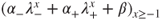 with
with 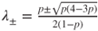 and for
  by
by 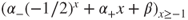 .
. - (d) Prove that if
 then
then 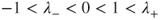 and if
  then
then  .
.
Deduce from this that, for
 , if
, if  then
then  and if
  then
then 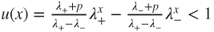 .
. - (e) Prove that
 satisfies
  and
and

Deduce from this that, for
 , if
, if  then
then  and if
  then
then 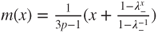 .
. - (f) What prevents us from computing the generating function of
 ?
?