
Chapter 1
First steps
1.1 Preliminaries
This book focuses on a class of random evolutions, in discrete time (by successive steps) on a discrete state space (finite or countable, with isolated elements), which satisfy a fundamental assumption, called the Markov property. This property can be described informally as follows: the evolution “forgets” its past and is “regenerated” at each step, retaining as sole past information for its future evolution its present state. The probabilistic description of such an evolution requires
- a law (probability measure) for drawing its initial state and
- a family of laws for drawing iteratively its state at the “next future instant” given its “present state,” indexed by the state space.
Such a random evolution will be called a Markov chain.
Precise definitions can be found in the Appendix, Section A.3, but we give now the probabilistic framework. A probability space ![]() will be considered throughout. When
will be considered throughout. When ![]() is discrete, usually its measurable structure is given by the collection of all subsets, and all functions with values in
is discrete, usually its measurable structure is given by the collection of all subsets, and all functions with values in ![]() are assumed to be measurable.
are assumed to be measurable.
A random variable (r.v.) with values in a measurable state space ![]() is a measurable function
is a measurable function
Intuitively, the output ![]() varies randomly with the input
varies randomly with the input ![]() , which is drawn in
, which is drawn in ![]() according to
according to ![]() , and the measurability assumptions allow to assign a probability to events defined through
, and the measurability assumptions allow to assign a probability to events defined through ![]() .
.
For the random evolutions under investigation, the natural random elements are sequences ![]() taking values in the same discrete state space
taking values in the same discrete state space ![]() , which are called (random) chains or (discrete time) processes. Each
, which are called (random) chains or (discrete time) processes. Each ![]() should be an r.v., and its law
should be an r.v., and its law ![]() on the discrete space
on the discrete space ![]() is then given by
is then given by

and hence can be identified in a natural way with ![]() .
.
Finite-dimensional marginals
More generally, for any ![]() and
and ![]() in
in ![]() , the random vector
, the random vector
takes values in the discrete space ![]() , and its law
, and its law ![]() can be identified with the collection of the
can be identified with the collection of the
All these laws for ![]() and
and ![]() constitute the family of the finite-dimensional marginals of the chain
constitute the family of the finite-dimensional marginals of the chain ![]() or of its law.
or of its law.
Law of the chain
The r.v.
takes values in ![]() , which is uncountable as soon as
, which is uncountable as soon as ![]() contains at least two elements. Hence, its law cannot, in general, be defined by the values it takes on the elements of
contains at least two elements. Hence, its law cannot, in general, be defined by the values it takes on the elements of ![]() . In the Appendix, Section A.3 contains some mathematical results defining the law of
. In the Appendix, Section A.3 contains some mathematical results defining the law of ![]() from its finite-dimensional marginals.
from its finite-dimensional marginals.
Section A.1 contains some more elementary mathematical results used throughout the book, and Section A.2 a discussion on the total variation norm and on weak convergence of laws.
1.2 First properties of Markov chains
1.2.1 Markov chains, finite-dimensional marginals, and laws
1.2.1.1 First definitions
We now provide rigorous definitions.
Markov chain evolution
A family ![]() of laws on
of laws on ![]() indexed by
indexed by ![]() is defined by
is defined by
The evolution of ![]() can be obtained by independent draws, first of
can be obtained by independent draws, first of ![]() according to
according to ![]() , and then iteratively of
, and then iteratively of ![]() according to
according to ![]() for
for ![]() without taking any further notice of the evolution before the present time
without taking any further notice of the evolution before the present time ![]() or of its actual value.
or of its actual value.
Inhomogeneous Markov chains
A more general and complex evolution can be obtained by letting the law of the steps depend on the present instant of time, that is, using the analogous formulae with ![]() instead of
instead of ![]() ; this corresponds to a time-inhomogeneous Markov chain, but we will seldom consider this generalization.
; this corresponds to a time-inhomogeneous Markov chain, but we will seldom consider this generalization.
Markov chain graph
The graph of the transition matrix ![]() , or of a Markov chain with matrix
, or of a Markov chain with matrix ![]() , is the oriented marked graph with nodes given by the elements of
, is the oriented marked graph with nodes given by the elements of ![]() and directed links given by the ordered pairs
and directed links given by the ordered pairs ![]() of elements of
of elements of ![]() such that
such that ![]() marked by the value of
marked by the value of ![]() . The restriction to the graph to
. The restriction to the graph to ![]() in
in ![]() is of the form [if
is of the form [if ![]() ]
]
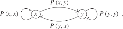
The graph and the matrix are equivalent descriptors for the random evolution. The links from ![]() to
to ![]() in the graph are redundant as they are marked by
in the graph are redundant as they are marked by ![]() , but illustrate graphically the possible transitions from
, but illustrate graphically the possible transitions from ![]() .
.
1.2.1.2 Conditional formulations
The last formula in Definition 1.2.1 can be written as
which is often used as the definition. Moreover, if ![]() is nonnegative or bounded then
is nonnegative or bounded then
For the sake of mathematical efficiency and simplicity, nonconditional expressions will be stressed, before possibly being translated into equivalent conditional formulations. As an example, Definition 1.2.1 immediately yields by summing over ![]() that
that
which is not quite so obvious starting from (1.2.1).
1.2.1.3 Initial law, instantaneous laws
For a Markov chain ![]() , the law of
, the law of ![]() of
of ![]() is called the instantaneous law at time
is called the instantaneous law at time ![]() and
and ![]() the initial law. The notations
the initial law. The notations ![]() and
and ![]() implicitly imply that
implicitly imply that ![]() is given and arbitrary,
is given and arbitrary, ![]() and
and ![]() for some law
for some law ![]() on
on ![]() indicate that
indicate that ![]() , and
, and ![]() and
and ![]() indicate that
indicate that ![]() . By linearity,
. By linearity,
A frequent abuse of notation is to write ![]() , and so on.
, and so on.
1.2.1.4 Law on the canonical space of the chain
The notions in the Appendix, Section A.3.4, will now be used.
Definition 1.2.1 is actually a statement on the law of the Markov chain ![]() , which it characterizes by giving an explicit expression for its finite-dimensional marginals in terms of its initial law
, which it characterizes by giving an explicit expression for its finite-dimensional marginals in terms of its initial law ![]() and transition matrix
and transition matrix ![]() .
.
Indeed, some rather simple results in measure theory show that there is uniqueness of a law on the canonical probability space ![]() with product
with product ![]() -field having a given finite-dimensional marginal collection.
-field having a given finite-dimensional marginal collection.
It is immediate to check that this collection is consistent [with respect to (w.r.t.) projections] and then the Kolmogorov extension theorem (Theorem A.3.10) implies that there is existence of a law ![]() on the canonical probability space
on the canonical probability space ![]() with the product
with the product ![]() -field such that the canonical (projection) process
-field such that the canonical (projection) process ![]() has the given finite-dimensional marginal collection, which hence is a Markov chain with initial law
has the given finite-dimensional marginal collection, which hence is a Markov chain with initial law ![]() and transition matrix
and transition matrix ![]() (see Corollary A.3.11).
(see Corollary A.3.11).
The Kolmogorov extension theorem follows from a deep and general result in measure theory, the Caratheodory extension theorem.
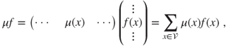
1.2.2 Transition matrix action and matrix notation
1.2.2.1 Nonnegative and signed measures, total variation measure, andnorm
A (nonnegative) measure ![]() on
on ![]() is defined by (and can be identified with) a collection
is defined by (and can be identified with) a collection ![]() of nonnegative real numbers and, in the sense of nonnegative series,
of nonnegative real numbers and, in the sense of nonnegative series,
A measure ![]() is finite if its total mass
is finite if its total mass ![]() is finite and then
is finite and then ![]() for all
for all ![]() . A measure is a probability measure, or a law, if
. A measure is a probability measure, or a law, if ![]() .
.
For ![]() in
in ![]() , let
, let ![]() and
and ![]() denote the nonnegative and nonpositive parts of
denote the nonnegative and nonpositive parts of ![]() , which satisfy
, which satisfy ![]() and
and ![]() .
.
For ![]() with
with ![]() , the measures
, the measures ![]() ,
, ![]() , and
, and ![]() can be defined term wise. Then,
can be defined term wise. Then,
is the minimal decomposition of ![]() as a difference of (nonnegative) measures, which have disjoint supports, and
as a difference of (nonnegative) measures, which have disjoint supports, and
is called the total variation measure of ![]() .
.
If ![]() is such that
is such that ![]() is finite (equivalently, if both
is finite (equivalently, if both ![]() and
and ![]() are finite), then we can extend it to a signed measure
are finite), then we can extend it to a signed measure ![]() acting on subsets of
acting on subsets of ![]() by setting, in the sense of absolutely converging series,
by setting, in the sense of absolutely converging series,
and we can define its total variation norm by
Note that ![]() for all
for all ![]() .
.
The space ![]() of all signed measures, furnished with the total variation norm, is a Banach space, which is isomorphic to the Banach space
of all signed measures, furnished with the total variation norm, is a Banach space, which is isomorphic to the Banach space ![]() of summable sequences with its natural norm.
of summable sequences with its natural norm.
Probability measures or laws
The space of probability measures
is the intersection of the cone of nonnegative measures with the unit sphere. It is a closed subset of ![]() and hence is complete for the induced metric.
and hence is complete for the induced metric.
Some properties of ![]() and
and ![]() are developed in the Appendix, Section A.2. Note that, according to the definition taken here, nonnegative measures with infinite mass are not signed measures.
are developed in the Appendix, Section A.2. Note that, according to the definition taken here, nonnegative measures with infinite mass are not signed measures.
Complex measures
Spectral theory naturally involves complex extensions. For its purposes, complex measures can be readily defined, and the corresponding space ![]() , where the modulus in
, where the modulus in ![]() is again denoted by
is again denoted by ![]() , allows to define a total variation measure
, allows to define a total variation measure ![]() and total variation norm
and total variation norm ![]() for
for ![]() in
in ![]() . The Banach space is isomorphic to
. The Banach space is isomorphic to ![]() . The real and imaginary parts of a complex measure are signed measures.
. The real and imaginary parts of a complex measure are signed measures.
1.2.2.2 Line and column vectors, measure-function duality
In matrix notation, the functions ![]() from
from ![]() to
to ![]() are considered as column vectors
are considered as column vectors ![]() , and nonnegative or signed measures
, and nonnegative or signed measures ![]() on
on ![]() as line vectors
as line vectors ![]() , of infinite lengths if
, of infinite lengths if ![]() is infinite. The integral of a function
is infinite. The integral of a function ![]() by a measure
by a measure ![]() is denoted by
is denoted by ![]() , in accordance with the matrix product
, in accordance with the matrix product
defined in ![]() in the sense of nonnegative series if
in the sense of nonnegative series if ![]() and
and ![]() and in
and in ![]() in the sense of absolutely converging series if
in the sense of absolutely converging series if ![]() and
and ![]() , the Banach space of bounded functions on
, the Banach space of bounded functions on ![]() with the uniform norm.
with the uniform norm.
For ![]() subset of
subset of ![]() , the indicator function
, the indicator function ![]() is defined by
is defined by
For ![]() in
in ![]() , the Dirac mass at
, the Dirac mass at ![]() is the probability measure
is the probability measure ![]() such that
such that ![]() , that is,
, that is,
For ![]() and
and ![]() in
in ![]() , it holds that
, it holds that
but ![]() will be represented by a line vector and
will be represented by a line vector and ![]() by a column vector.
by a column vector.
If ![]() is a nonnegative or signed measure, then
is a nonnegative or signed measure, then
Duality and total variation norm
A natural duality bracket between the Banach spaces ![]() and
and ![]() is given by
is given by
and for ![]() in
in ![]() , it holds that
, it holds that
and hence that
Thus, ![]() can be identified with a closed subspace of the dual of
can be identified with a closed subspace of the dual of ![]() with the strong dual norm, which is the norm as an operator on
with the strong dual norm, which is the norm as an operator on ![]() .
.
The space ![]() can be identified with the space
can be identified with the space ![]() of bounded sequences, and this duality between
of bounded sequences, and this duality between ![]() and
and ![]() to the natural duality between
to the natural duality between ![]() and
and ![]() .
.
The operations between complex measures and complex functions are performed by separating the real and imaginary parts.
1.2.2.3 Transition matrices, actions on measures, and functions
A matrix ![]() is a transition matrix if and only if each of its line vectors
is a transition matrix if and only if each of its line vectors ![]() corresponds to a probability measure. Then, its column vector
corresponds to a probability measure. Then, its column vector ![]() defines a nonnegative function, which is bounded by
defines a nonnegative function, which is bounded by ![]() .
.
A transition matrix can be multiplied on its right by nonnegative functions and on its left by nonnegative measures, or on its right by bounded functions and on its left by signed measures. The order of these operations does not matter. The function ![]() , the nonnegative or signed measure
, the nonnegative or signed measure ![]() , and
, and ![]() are given for
are given for ![]() by
by
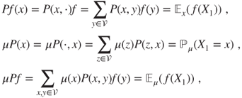
in which the notations ![]() and
and ![]() are used only when
are used only when ![]() is a law.
is a law.
In matrix notation,
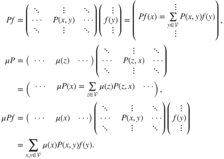
Intrinsic notation
The linear mapping
has matrix ![]() in the canonical basis. Its dual, or adjoint, mapping on
in the canonical basis. Its dual, or adjoint, mapping on ![]() , w.r.t. the duality bracket
, w.r.t. the duality bracket ![]() , is given by
, is given by
and has the adjoint (or transpose) matrix, also denoted by ![]() . In order to respect the vector space structure and identify linear mappings and their matrices in the canonical bases, we could write
. In order to respect the vector space structure and identify linear mappings and their matrices in the canonical bases, we could write ![]() instead of
instead of ![]() and
and ![]() instead of
instead of ![]() and
and ![]() instead of
instead of ![]() .
.
1.2.2.4 Transition matrix products, many-step transition
If ![]() and
and ![]() are both transition matrices on
are both transition matrices on ![]() , then it is easy to check that the matrix product
, then it is easy to check that the matrix product ![]() with generic term
with generic term
is a transition matrix on ![]() . Let
. Let
Then,
is the probability for ![]() to go in one step from
to go in one step from ![]() to
to ![]() , and hence for
, and hence for ![]() to do so in
to do so in ![]() steps. In particular,
steps. In particular,
Chapman–Kolmogorov formula
As ![]() for
for ![]() , this yields the Chapman–Kolmogorov formula
, this yields the Chapman–Kolmogorov formula
Probabilistic interpretation
These algebraic formulae have simple probabilistic interpretations: the probability of going from ![]() to
to ![]() in
in ![]() steps can be obtained as the sum of the probabilities of taking every
steps can be obtained as the sum of the probabilities of taking every ![]() -step path allowing to do so, as well as the sum over all intermediate positions after
-step path allowing to do so, as well as the sum over all intermediate positions after ![]() steps.
steps.
1.2.3 Random recursion and simulation
Many Markov chains are obtained in a natural way as a random recursion, or random iterative sequence, as follows.
When a random sequence ![]() is defined in some particular way, there is often a natural interpretation in terms of a random recursion of the previous kind. This allows to prove that a
is defined in some particular way, there is often a natural interpretation in terms of a random recursion of the previous kind. This allows to prove that a ![]() is a Markov chain, without having to directly check the definition, or even having to explicit its matrix. Moreover, such a pathwise representation for the Markov chain may be used for its study or its simulation.
is a Markov chain, without having to directly check the definition, or even having to explicit its matrix. Moreover, such a pathwise representation for the Markov chain may be used for its study or its simulation.
Any Markov chain, with arbitrary initial law ![]() and transition matrix
and transition matrix ![]() , can be thus represented, using an i.i.d. sequence
, can be thus represented, using an i.i.d. sequence ![]() of uniform r.v. on
of uniform r.v. on ![]() . The state space is first enumerated as
. The state space is first enumerated as ![]() .
.
Let ![]() . For the initial value, if
. For the initial value, if ![]() is determined by
is determined by
then ![]() . For the transitions, for
. For the transitions, for ![]() , if
, if ![]() is determined by
is determined by
then ![]() .
.
In theory, this allows for the simulation of the Markov chain, but in practice this is not necessarily the best way to do so.
Note that this representation yields a construction for an arbitrary Markov chain, starting from a rigorous construction of i.i.d. sequences of uniform r.v. on ![]() , without having to use the more general Kolmogorov extension theorem (Theorem A.3.10).
, without having to use the more general Kolmogorov extension theorem (Theorem A.3.10).
1.2.4 Recursion for the instantaneous laws, invariant laws
The instantaneous laws ![]() satisfy the recursion
satisfy the recursion
with solution ![]() . This is a linear recursion in dimension
. This is a linear recursion in dimension ![]() , and the affine constraint
, and the affine constraint ![]() allows to reduce it to an affine recursion in dimension
allows to reduce it to an affine recursion in dimension ![]() . Note that
. Note that ![]() for
for ![]() .
.
An elementary study of this recursion starts by searching for its fixed points. These are the only possible large ![]() limits for the instantaneous laws, for any topology such that
limits for the instantaneous laws, for any topology such that ![]() is continuous.
is continuous.
By definition, a fixed point for this recursion is a law (probability measure) ![]() such that
such that ![]() , and is called an invariant law or a stationary distribution for (or of) the matrix
, and is called an invariant law or a stationary distribution for (or of) the matrix ![]() , or the Markov chain
, or the Markov chain ![]() .
.
Stationary chain, equilibrium
If ![]() is an invariant law and
is an invariant law and ![]() , then
, then ![]() for all
for all ![]() in
in ![]() , and
, and ![]() is again a Markov chain with initial law
is again a Markov chain with initial law ![]() and transition matrix
and transition matrix ![]() . Then,
. Then, ![]() is said to be stationary, or in equilibrium.
is said to be stationary, or in equilibrium.
Invariant measures and laws
In order to find an invariant law, one must:
- Solve the linear equation
 .
. - Find which solutions
 are nonnegative, that is, such that
  .
. - Normalize such
 by setting
  , which is possible only if

A nonnegative measure ![]() such that
such that ![]() is called an invariant measure. An invariant measure is said to be unique if it is unique up to a multiplicative factor, that is, if all invariant measures are proportional (to it).
is called an invariant measure. An invariant measure is said to be unique if it is unique up to a multiplicative factor, that is, if all invariant measures are proportional (to it).
Algebraic interpretation
The invariant measures are the left eigenvectors for the eigenvalue 1 for the matrix ![]() acting on nonnegative measures, that is, for the adjoint (or transposed) matrix
acting on nonnegative measures, that is, for the adjoint (or transposed) matrix ![]() acting on nonnegative vectors. Note that the constant function
acting on nonnegative vectors. Note that the constant function ![]() is a right eigenvector for the eigenvalue
is a right eigenvector for the eigenvalue ![]() , as
, as
The possible convergence of ![]() to an invariant law
to an invariant law ![]() is related to the moduli of the elements of the spectrum of the restriction of the action of
is related to the moduli of the elements of the spectrum of the restriction of the action of ![]() on the signed measures of null total mass.
on the signed measures of null total mass.
More generally, the exact or approximate computation of ![]() depends in a more or less explicit way on a spectral decomposition of
depends in a more or less explicit way on a spectral decomposition of ![]() .
.