
Chapter 2
Past, present, and future
2.1 Markov property and its extensions
2.1.1 Past  -field, filtration, and translation operators
Let ![]() be a sequence of random variables. The
be a sequence of random variables. The ![]() -fields
-fields
contain all events that can be observed using exclusively ![]() , that is, the past up to time
, that is, the past up to time ![]() included of the sequence. Obviously
included of the sequence. Obviously
A family of nondecreasing ![]() -fields, such as
-fields, such as ![]() , is called a filtration, and provides a mathematical framework for the accumulation of information obtained by the step-by-step observation of the sequence.
, is called a filtration, and provides a mathematical framework for the accumulation of information obtained by the step-by-step observation of the sequence.
Product  -field
Definition 1.2.1 gives an expression for the probability of any event ![]() in
in ![]() in terms of
in terms of ![]() and
and ![]() . The Kolmogorov extension theorem (Theorem A.3.10) in Section A.3.4 of the Appendix then attributes a corresponding probability to any event in the product
. The Kolmogorov extension theorem (Theorem A.3.10) in Section A.3.4 of the Appendix then attributes a corresponding probability to any event in the product ![]() -field of
-field of ![]() , which is the smallest
, which is the smallest ![]() -field containing every
-field containing every ![]() , which we denote by
, which we denote by ![]() . The
. The ![]() -field
-field ![]() contains all the information that can be reconstructed from the observation of an arbitrarily large finite number of terms of the sequence
contains all the information that can be reconstructed from the observation of an arbitrarily large finite number of terms of the sequence ![]() .
.
As a ![]() -field is stable under countable intersections,
-field is stable under countable intersections, ![]() contains events allowing to characterize a.s. convergences, of which we will discuss later.
contains events allowing to characterize a.s. convergences, of which we will discuss later.
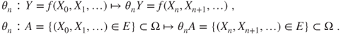
Shift operators
For ![]() , the shift operators
, the shift operators ![]() act on sequences of r.v. by
act on sequences of r.v. by
This action extends naturally to any ![]() -measurable random variable
-measurable random variable ![]() and to any event
and to any event ![]() in
in ![]() : if
: if ![]() and
and ![]() for some measurable (deterministic) function
for some measurable (deterministic) function ![]() on
on ![]() and measurable subset
and measurable subset ![]() , then
, then
The ![]() -field
-field ![]() is included in
is included in ![]() and contains the events of the future after time
and contains the events of the future after time ![]() included for the sequence. It corresponds for
included for the sequence. It corresponds for ![]() to what
to what ![]() corresponds for
corresponds for ![]() .
.
2.1.2 Markov property
Definition 1.2.1 is in fact equivalent to the following Markov property, which is apparently stronger as it yields that the past and the future of a Markov chain are independent conditional on its present state.
Thus, conditional to ![]() , the future after time
, the future after time ![]() of the chain is given by a “regeneration” of the chain starting at
of the chain is given by a “regeneration” of the chain starting at ![]() and independent of the past. Note that past and future are taken in wide sense and include the present: both
and independent of the past. Note that past and future are taken in wide sense and include the present: both ![]() and
and ![]() may contain information on
may contain information on ![]() “superseded” by the conditioning on
“superseded” by the conditioning on ![]() . All this is illustrated by Figure 2.1, for
. All this is illustrated by Figure 2.1, for ![]() .
.

Figure 2.1 Strong Markov property. The successive states of  are represented by the filled circles and are linearly interpolated by dashed lines and
  is a stopping time.
These formulae are compact, have rich interpretations, and can readily be extended, for instance, if ![]() and
and ![]() are nonnegative or bounded then
are nonnegative or bounded then
We now proceed to further extend them by replacing deterministic instants ![]() by an adequate class of random instants.
by an adequate class of random instants.
2.1.3 Stopping times and strong Markov property
A stopping time will be defined as a random instant that can be determined “in real time” from the observation of the chain, and hence at which a decision (such as stopping a game) can be taken without further knowledge of the future.
The equivalences in the definition follow readily from
We set ![]() and
and ![]() on
on ![]() . On
. On ![]() , it holds that, for
, it holds that, for ![]() ,
,
For ![]() , it holds that
, it holds that ![]() , and for any
, and for any ![]() , one can determine whether a certain
, one can determine whether a certain ![]() is in
is in ![]() by examining only
by examining only ![]() .
.
Trivial example: deterministic times
If ![]() is deterministic, that is, if
is deterministic, that is, if
then ![]() is a stopping time and
is a stopping time and ![]() .
.
We shall give nontrivial examples of stopping times after the next fundamental result, illustrated in Figure 2.1, which yields that Theorem 2.1.1 and its corollaries, such as (2.1.1), hold conditionally on ![]() by replacing
by replacing ![]() with a stopping time
with a stopping time ![]() .
.
A “last hitting time,” a “time of maximum,” and so on are generally not stopping times, as the future knowledge they imply usually prevents the formula for the strong Markov property to hold.
2.2 Hitting times and distribution
2.2.1 Hitting times, induced chain, and hitting distribution
2.2.1.1 First hitting time and first strict future hitting time
Let ![]() be a subset of
be a subset of ![]() . The r.v., with values in
. The r.v., with values in ![]() , defined by
, defined by
are stopping times, as ![]() and
and ![]() . Clearly,
. Clearly,
When ![]() , the notations
, the notations ![]() and
and ![]() are used. The notations
are used. The notations ![]() and
and ![]() or
or ![]() and
and ![]() , or even
, or even ![]() and
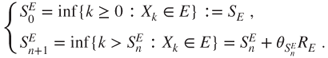
and ![]() if the contest is clear, will also be used. See Figure 2.2 in which
if the contest is clear, will also be used. See Figure 2.2 in which ![]() .
.
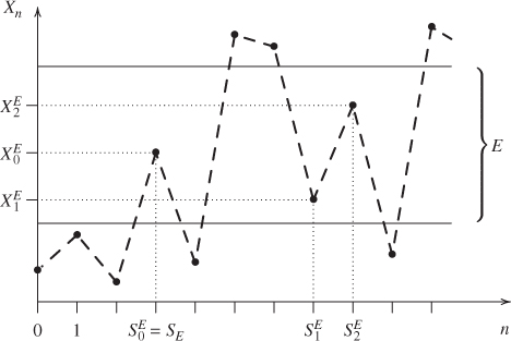
Figure 2.2 Successive hitting times of  and induced chain. The successive states of
  are represented by the filled circles and are linearly interpolated, and
  corresponds to the points between the two horizontal lines. We see
  for
for  ,
,  , and
, and  .
.
Classically, ![]() is called the (first) hitting time of
is called the (first) hitting time of ![]() by the chain and
by the chain and ![]() the (first) strict future hitting time of
the (first) strict future hitting time of ![]() by the chain.
by the chain.
2.2.1.2 Successive hitting times and induced chain
The successive hitting times ![]() of
of ![]() by the chain
by the chain ![]() are given by
are given by
These are stopping times, as ![]() .
.
If ![]() then we set
then we set ![]() , which is the state occupied at the
, which is the state occupied at the ![]() th hit of
th hit of ![]() by the chain. This is illustrated in Figure 2.2.
by the chain. This is illustrated in Figure 2.2.
If ![]() for every
for every ![]() , then
, then ![]() is said to be recurrent. Then, the strong Markov property (Theorem 2.1.3) yields that if
is said to be recurrent. Then, the strong Markov property (Theorem 2.1.3) yields that if ![]() , for instance, if
, for instance, if ![]() a.s., then
a.s., then ![]() for all
for all ![]() , and moreover that
, and moreover that ![]() is a Markov chain on
is a Markov chain on ![]() , which is called the induced chain of
, which is called the induced chain of ![]() in
in ![]() .
.
Cemetery state
In order to define ![]() in all generality, we can set
in all generality, we can set ![]() if
if ![]() for a cemetery state
for a cemetery state ![]() adjoined to
adjoined to ![]() . The strong Markov property implies that
. The strong Markov property implies that ![]() thus defined is a Markov chain on the enlarged state space
thus defined is a Markov chain on the enlarged state space ![]() , also called the induced chain; one can add that it is killed after its last hit of
, also called the induced chain; one can add that it is killed after its last hit of ![]() .
.
2.2.1.3 Hitting distribution and induced chain
For ![]() , the matrix and function
, the matrix and function
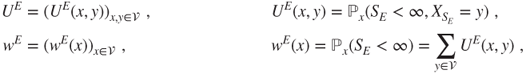
only depend on ![]() and on
and on ![]() as the starting states are specified. When
as the starting states are specified. When ![]() , the notations
, the notations ![]() and
and ![]() are used, and
are used, and ![]() and
and ![]() when the context is clear.
when the context is clear.
Clearly, ![]() for
for ![]() and
and ![]() is sub-Markovian (nonnegative terms, sum of each line bounded by
is sub-Markovian (nonnegative terms, sum of each line bounded by ![]() ) and is Markovian if and only if
) and is Markovian if and only if ![]() .
.
The restriction of ![]() to
to ![]() is Markovian if and only if
is Markovian if and only if ![]() is recurrent and then it is the transition matrix of the induced chain
is recurrent and then it is the transition matrix of the induced chain ![]() . Else, a Markovian extension of
. Else, a Markovian extension of ![]() is obtained using a cemetery state
is obtained using a cemetery state ![]() adjoined to
adjoined to ![]() , and setting
, and setting ![]() for
for ![]() in
in ![]() and
and ![]() ; its restriction to
; its restriction to ![]() is the transition matrix of the induced chain on the extended state space. The matrix of the chain conditioned to return to
is the transition matrix of the induced chain on the extended state space. The matrix of the chain conditioned to return to ![]() is given by
is given by ![]() .
.
The matrix notation conventions in Section 1.2.2 are used for ![]() . For
. For ![]() in
in ![]() , the line vector
, the line vector ![]() is a subprobability measure, with support
is a subprobability measure, with support ![]() and total mass
and total mass ![]() , called the (possibly defective) hitting distribution of
, called the (possibly defective) hitting distribution of ![]() starting from
starting from ![]() . It associates to
. It associates to ![]() the quantity
the quantity
For ![]() or
or ![]() , the function
, the function ![]() is given for
is given for ![]() by
by
and this can be extended to signed bounded functions, by setting
Clearly, ![]() and
and ![]() and
and ![]() . If
. If ![]() then
then ![]() and in particular
and in particular ![]() and
and ![]() .
.
2.2.2 “One step forward” method, Dirichlet problem
2.2.2.1 General principle
Let ![]() be a Markov chain with matrix
be a Markov chain with matrix ![]() . The Markov property (Theorem 2.1.1) yields that the shifted chain by one step
. The Markov property (Theorem 2.1.1) yields that the shifted chain by one step
is also a Markov chain with matrix ![]() and that conditional on
and that conditional on ![]() it is started at
it is started at ![]() and independent of
and independent of ![]() . This is illustrated in Figure 2.1, with
. This is illustrated in Figure 2.1, with ![]() .
.
The “one step forward” method
The “one step forward” method, or the method of conditioning on the first step, exploits this fact. It consists in rewriting quantities of interest for ![]() in terms of the shifted chain
in terms of the shifted chain ![]() and then using the above observation to establish equations for these quantities. These equations can then be solved or studied qualitatively and quantitatively.
and then using the above observation to establish equations for these quantities. These equations can then be solved or studied qualitatively and quantitatively.
A natural framework for this method is the study of hitting times and locations of ![]() , as:
, as:
- the hitting time
 is a function of
  , and
, and  the same function of
 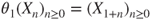 ;
; - if
 then
then  and
and  and if
  then
then  and
and  on
on  .
.
2.2.2.2 Hitting distribution and Dirichlet problem
This method will provide an equation for ![]() , which we are going to study.
, which we are going to study.
All that matters about ![]() is its restriction to the boundary of
is its restriction to the boundary of ![]() for
for ![]() given by
given by
and the solution is the null extension of ![]() .
.
The r.v. ![]() and subprobability measure
and subprobability measure ![]() are also called the exit time and distribution of
are also called the exit time and distribution of ![]() by the chain, and one must take care about notation.
by the chain, and one must take care about notation.
Dirichlet problem and recurrence
A direct consequence of Theorem 2.2.2 is that an irreducible Markov chain on a finite state space hits every state ![]() starting from any state
starting from any state ![]() , a.s., as irreducibility implies that
, a.s., as irreducibility implies that ![]() for all
for all ![]() and hence that
and hence that ![]() , and the theorem yields that
, and the theorem yields that ![]() . The strong Markov property implies that if
. The strong Markov property implies that if ![]() for all
for all ![]() , then the Markov chain visits every state infinitely often, a.s.
, then the Markov chain visits every state infinitely often, a.s.
We give a more general result. A subset ![]() of
of ![]() communicates with another subset
communicates with another subset ![]() of
of ![]() if for every
if for every ![]() there exists
there exists ![]() and
and ![]() such that
such that ![]() . This is always the case if
. This is always the case if ![]() is irreducible and
is irreducible and ![]() is nonempty.
is nonempty.
2.2.2.3 Generating functions, joint distribution of hitting time, and location
Let ![]() be nonempty. In order to study the (defective) joint distribution of
be nonempty. In order to study the (defective) joint distribution of ![]() and
and ![]() , consider for
, consider for ![]() , and
, and ![]() the generating functions given for
the generating functions given for ![]() by
by
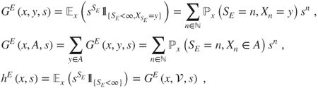
which depend only on the matrix ![]() of the chain. Clearly,
of the chain. Clearly,
The notations ![]() and
and ![]() are used for
are used for ![]() , and
, and ![]() and
and ![]() when the context is clear. Then
when the context is clear. Then
which allows to study the condition law of ![]() given
given ![]() and
and ![]() .
.
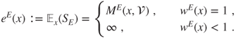
2.2.2.4 Direct computations for expectations
For ![]() and
and ![]() , we have
, we have

Nevertheless, it may be best to work directly on ![]() and
and ![]() , and possibly one may be able to solve the corresponding equations and not those for
, and possibly one may be able to solve the corresponding equations and not those for ![]() . Let
. Let
The notations ![]() and
and ![]() are used for
are used for ![]() , and
, and ![]() and
and ![]() if the context is clear.
if the context is clear.
The “right-hand side” ![]() or
or ![]() of the affine equation is a solution of the associated linear equation, which corresponds to the Dirichlet problem (2.2.5). This fact can be exploited to find a particular solution of the affine equation.
of the affine equation is a solution of the associated linear equation, which corresponds to the Dirichlet problem (2.2.5). This fact can be exploited to find a particular solution of the affine equation.
2.3 Detailed examples
The results in this section will be now applied to some quantities of interest for the detailed examples described in Section 1.4. The main idea will be to solve the equations derived by the “one step forward” method, using the results obtained on the Dirichlet problem and related equations when appropriate.
The description of the Monte Carlo method for the approximate solution of the Dirichlet problem is left for Section 5.1.
2.3.1 Gambler's ruin
See Section 1.4.2. Here ![]() and
and ![]() , and the game duration is
, and the game duration is ![]() . We set
. We set ![]() . Gambler A is ruined if
. Gambler A is ruined if ![]() and then Gambler B wins. There is a symmetry between the gamblers by interchanging
and then Gambler B wins. There is a symmetry between the gamblers by interchanging ![]() with
with ![]() and
and ![]() with
with ![]() .
.
2.3.1.1 Finite game and ruin probability
Starting from an initial fortune of ![]() , the probability of eventual ruin and eventual win of Gambler A are given by
, the probability of eventual ruin and eventual win of Gambler A are given by
and the probability that the game eventually terminates by
Proposition 2.2.4 implies that ![]() , but a direct proof will be provided.
, but a direct proof will be provided.
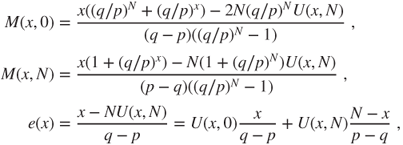
Theorem 2.2.2 (or a direct implementation of the “one step forward” method) yields that ![]() and
and ![]() and
and ![]() are solutions of
are solutions of
with respective boundary conditions ![]() and
and ![]() ,
, ![]() and
and ![]() , and
, and ![]() .
.
This is a linear second-order recursion, with characteristic polynomial
with roots ![]() and
and ![]() , which can possibly be equal.
, which can possibly be equal.
Biased game
This is the case ![]() , in which the roots are distinct. The general solution is given by
, in which the roots are distinct. The general solution is given by ![]() , hence
, hence ![]() and
and
Fair game
This is the case ![]() , in which
, in which ![]() is a double root. The general solution is given by
is a double root. The general solution is given by ![]() , hence
, hence ![]() and
and
These are the limits for ![]() going to
going to ![]() of the values for the biased game.
of the values for the biased game.
2.3.1.2 Mean game duration
Theorem 2.2.6 yields that the function ![]() for
for ![]() satisfies
satisfies
with ![]() and that
and that ![]() satisfies the same equation in which
satisfies the same equation in which ![]() is replaced by
is replaced by ![]() .
.
The general solution of such an affine equation is given by the sum of a particular solution and of the general solution to the related linear equation (2.3.7), the latter being already known. The r.h.s. ![]() is one of these general solutions, a fact to be exploited in order to find a particular solution.
is one of these general solutions, a fact to be exploited in order to find a particular solution.
Biased game
A particular solution of the form ![]() satisfies
satisfies
which yields for the r.h.s. ![]() that
that ![]() and
and ![]() , for
, for ![]() that
that ![]() , and for
, and for ![]() that
that ![]() and
and ![]() , the sum of the previous quantities. The null boundary conditions allow to conclude that
, the sum of the previous quantities. The null boundary conditions allow to conclude that
as soon as we have eliminated the possibility of infinite solutions. This is a delicate point in Theorem 2.2.6, see the remark thereafter.
As ![]() is finite, Proposition 2.2.4 allows to conclude. A more direct proof is that the solution for the r.h.s.
is finite, Proposition 2.2.4 allows to conclude. A more direct proof is that the solution for the r.h.s. ![]() (the formula for
(the formula for ![]() ) is nondecreasing from the value
) is nondecreasing from the value ![]() at state
at state ![]() to a certain state, then is nonincreasing down to the value
to a certain state, then is nonincreasing down to the value ![]() at state
at state ![]() , and hence is nonnegative, and the minimality result in Theorem 2.2.6 allows to eliminate the infinite solution.
, and hence is nonnegative, and the minimality result in Theorem 2.2.6 allows to eliminate the infinite solution.
It can be noted that ![]() is the mean, weighted by the probabilities of ruin and of win, of two quantities of opposite signs, which essentially correspond to a motion with speed
is the mean, weighted by the probabilities of ruin and of win, of two quantities of opposite signs, which essentially correspond to a motion with speed ![]() . This is called a ballistic phenomenon.
. This is called a ballistic phenomenon.
Fair game
A particular solution of the form ![]() satisfies
satisfies
which yields for ![]() that
that ![]() and
and ![]() , for
, for ![]() that
that ![]() and
and ![]() , and for
, and for ![]() that
that ![]() and
and ![]() (the sums). The null boundary conditions allow to conclude that
(the sums). The null boundary conditions allow to conclude that
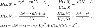
where the infinite solution can be eliminated by Proposition 2.2.4 or remarking that these solutions are nonnegative.
The mean time taken to reach a distance ![]() is of order
is of order ![]() , which corresponds to a diffusive phenomenon.
, which corresponds to a diffusive phenomenon.