
1.3 Natural duality: algebraic approach
An algebraic study based on the natural duality between the space of signed measures ![]() and the space of bounded functions
and the space of bounded functions ![]() will provide some structural results. These results are quite complete for finite state spaces
will provide some structural results. These results are quite complete for finite state spaces ![]() . The complete study for arbitrary discrete
. The complete study for arbitrary discrete ![]() will be done later using probabilistic techniques. A reader for which this is the main interest may go directly to Section 1.4.
will be done later using probabilistic techniques. A reader for which this is the main interest may go directly to Section 1.4.
1.3.1 Complex eigenvalues and spectrum
1.3.1.1 Some reminders
The eigenvalues of the operator
are given by all ![]() such that
such that ![]() is not injective as an operator on
is not injective as an operator on ![]() .
.
The eigenspace of ![]() is the kernel
is the kernel
and its nonzero elements are called eigenvectors. Hence, ![]() in
in ![]() is an eigenvector of
is an eigenvector of ![]() if and only if
if and only if
and then
The generalized eigenspace of ![]() is given by
is given by
If it contains strictly the eigenspace, then it contains some ![]() and some eigenvector
and some eigenvector ![]() such that
such that
and then
An eigenvalue is said to be
- semisimple if the eigenspace and generalized eigenspace coincide,
- simple if these spaces have dimension
 .
.
Similar definitions involving ![]() are given for the adjoint operator
are given for the adjoint operator
Its eigenspaces are often said to be eigenspaces on the left, or left eigenspaces, of ![]() . Those of
. Those of
may accordingly be called eigenspaces on the right, or right eigenspaces, of ![]() .
.
Hence, ![]() is a left eigenvector of
is a left eigenvector of ![]() if and only if
if and only if
and then
If the generalized left eigenspace of ![]() contains strictly the eigenspace, then it contains some
contains strictly the eigenspace, then it contains some ![]() and some left eigenvector
and some left eigenvector ![]() such that
such that
and then
The spectrum ![]() of
of ![]() on
on ![]() is given by
is given by
It is a simple matter to check that, using ![]() in the definition,
in the definition,
and mentions of “left” or “right” are useless.
The spectrum ![]() contains both the left and right eigenvectors. In finite dimensions, invertibility of an operator is the same as injectivity, and hence the spectrum, the left eigenspace, and the right eigenspace coincide, but it is not so in general.
contains both the left and right eigenvectors. In finite dimensions, invertibility of an operator is the same as injectivity, and hence the spectrum, the left eigenspace, and the right eigenspace coincide, but it is not so in general.
If ![]() is in the spectrum of an operator on a real vector space, such as
is in the spectrum of an operator on a real vector space, such as ![]() or
or ![]() , then
, then ![]() is also in the spectrum, and if moreover
is also in the spectrum, and if moreover ![]() is an eigenvalue, then
is an eigenvalue, then ![]() is an eigenvalue, and the corresponding (generalized) eigenspaces are conjugate.
is an eigenvalue, and the corresponding (generalized) eigenspaces are conjugate.
If ![]() , then
, then ![]() can be considered instead of
can be considered instead of ![]() in all definitions. Moreover, the real and complex (generalized) eigenspaces have same dimension.
in all definitions. Moreover, the real and complex (generalized) eigenspaces have same dimension.
1.3.1.2 Algebraic results for transition matrices
1.3.1.3 Uniqueness for invariant laws and irreducibility
A state ![]() in
in ![]() is absorbing if
is absorbing if ![]() and then
and then ![]() is an invariant law for
is an invariant law for ![]() .
.
If ![]() contains subsets
contains subsets ![]() for
for ![]() such that
such that ![]() for every
for every ![]() , these are said to be absorbing or closed. The restriction of
, these are said to be absorbing or closed. The restriction of ![]() to each
to each ![]() is Markovian; if it has an invariant measure
is Markovian; if it has an invariant measure ![]() , then any convex combination
, then any convex combination ![]() is an invariant measure on
is an invariant measure on ![]() , and if the
, and if the ![]() are laws then
are laws then ![]() is an invariant law. (By abuse of notation,
is an invariant law. (By abuse of notation, ![]() denotes the extension of the measure to
denotes the extension of the measure to ![]() vanishing outside of
vanishing outside of ![]() .)
.)
Hence, any uniqueness result for invariant measures or laws requires adequate assumptions excluding the above situation.
The standard hypothesis for this is that of irreducibility: a transition matrix ![]() on
on ![]() is irreducible if, for every
is irreducible if, for every ![]() and
and ![]() in
in ![]() , there exists
, there exists ![]() such that
such that ![]() . Equivalently, there exists in the oriented graph of the matrix a path covering the whole graph (respecting orientation). This notion will be further developed in due time.
. Equivalently, there exists in the oriented graph of the matrix a path covering the whole graph (respecting orientation). This notion will be further developed in due time.
This proof heavily uses techniques that are referred under the terminology “the maximum principle,” which we will try to explain in Section 1.3.3.
1.3.2 Doeblin condition and strong irreducibility
A transition matrix ![]() is strongly irreducible if there exists
is strongly irreducible if there exists ![]() such that
such that ![]() .
.
Note that ![]() and that
and that ![]() only in the trivial case in which
only in the trivial case in which ![]() is a sequence of i.i.d. r.v. of law
is a sequence of i.i.d. r.v. of law ![]() .
.
The Doeblin Condition (or strong irreducibility) is seldom satisfied when the state space ![]() is infinite. For a finite state space, Section 4.2.1 will give verifiable conditions for strong irreducibility. The following result is interesting in these perspectives.
is infinite. For a finite state space, Section 4.2.1 will give verifiable conditions for strong irreducibility. The following result is interesting in these perspectives.
1.3.3 Finite state space Markov chains
1.3.3.1 Perron–Frobenius theorem
If the state space ![]() is finite, then the vector spaces
is finite, then the vector spaces ![]() and
and ![]() have finite dimension
have finite dimension ![]() .
.
Then, the eigenvalues and the dimensions of the eigenspaces and generalized eigenspaces of ![]() , which are by definition those of
, which are by definition those of ![]() and
and ![]() , are identical, and the spectrum is constituted of the eigenvalues.
, are identical, and the spectrum is constituted of the eigenvalues.
A function ![]() is harmonic if
is harmonic if ![]() . It is a right eigenvector for the eigenvalue
. It is a right eigenvector for the eigenvalue ![]() .
.
Theorem 4.2.7 will provide an extension of these results for infinite ![]() , by wholly different methods. (Saloff-Coste, L. (1997), Section 1.2) provides a detailed commentary on the Doeblin condition and the Perron–Frobenius theorem.
, by wholly different methods. (Saloff-Coste, L. (1997), Section 1.2) provides a detailed commentary on the Doeblin condition and the Perron–Frobenius theorem.
Maximum principle
This terminology comes from the following short direct proof of the fact that if the state space ![]() is finite and
is finite and ![]() is irreducible, then every harmonic function is constant. If
is irreducible, then every harmonic function is constant. If ![]() is harmonic on
is harmonic on ![]() , then it attains its maximum in at least a state
, then it attains its maximum in at least a state ![]() . Moreover,
. Moreover,
and as ![]() is a probability measure,
is a probability measure, ![]() for all
for all ![]() such that
such that ![]() . Thus, irreducibility yields that
. Thus, irreducibility yields that ![]() for every
for every ![]() , and thus that
, and thus that ![]() is constant.
is constant.
1.3.3.2 Computation of the instantaneous and invariant laws
We are now going to solve the recursion for the instantaneous laws ![]() , and see how the situation deteriorates in practice very quickly as the size of the state space increases.
, and see how the situation deteriorates in practice very quickly as the size of the state space increases.
The chain with two states
Let us denote the states by ![]() and
and ![]() . There exists
. There exists ![]() such that the transition matrix
such that the transition matrix ![]() and its graph are given by
and its graph are given by
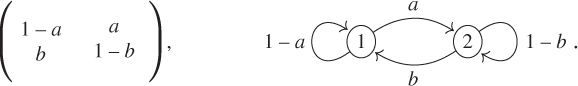
The recursion formula ![]() then writes
then writes
and the affine constraint ![]() allows to reduce this linear recursion in dimension
allows to reduce this linear recursion in dimension ![]() to the affine recursion, in dimension
to the affine recursion, in dimension ![]() ,
,
If ![]() , then
, then ![]() and every law is invariant, and
and every law is invariant, and ![]() is not irreducible as
is not irreducible as ![]() . Else, the unique fixed point is
. Else, the unique fixed point is ![]() , the unique invariant law is
, the unique invariant law is ![]() , and
, and
and the formula for ![]() is obtained by symmetry or as
is obtained by symmetry or as ![]() .
.
If ![]() , then
, then ![]() has eigenvalues
has eigenvalues ![]() and
and ![]() , the latter with eigenvector
, the latter with eigenvector ![]() , and the chain alternates between the states
, and the chain alternates between the states ![]() and
and ![]() and
and ![]() is equal to
is equal to ![]() for even
for even ![]() and to
and to ![]() for odd
for odd ![]() .
.
If ![]() , then
, then ![]() and
and ![]() with geometric rate with reason
with geometric rate with reason ![]() .
.
The chain with three states
Let us denote the states by ![]() ,
, ![]() , and
, and ![]() . There exists
. There exists ![]() ,
, ![]() ,
, ![]() ,
, ![]() ,
, ![]() , and
, and ![]() in
in ![]() , satisfying
, satisfying ![]() ,
, ![]() , and
, and ![]() , such that the transition matrix
, such that the transition matrix ![]() and its graph are given by
and its graph are given by
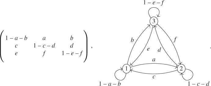
As discussed above, we could reduce the linear recursion in dimension ![]() to an affine recursion in dimension
to an affine recursion in dimension ![]() . Instead, we give the elements of a vectorial computation in dimension
. Instead, we give the elements of a vectorial computation in dimension ![]() , which can be generalized to all dimensions. This exploits the fact that
, which can be generalized to all dimensions. This exploits the fact that ![]() is an eigenvalue of
is an eigenvalue of ![]() and hence a root of its characteristic polynomial
and hence a root of its characteristic polynomial ![]() . Hence,
. Hence,

and by developing this polynomial and using the fact that ![]() is a root,
is a root, ![]() factorizes into
factorizes into

The polynomial of degree ![]() is the characteristic polynomial of the affine recursion in dimension
is the characteristic polynomial of the affine recursion in dimension ![]() . It has two possible equal roots
. It has two possible equal roots ![]() and
and ![]() in
in ![]() , and if
, and if ![]() , then
, then ![]() . Their exact theoretical expression is not very simple, as the discriminant of this polynomial does not simplify in general, but they can easily be computed on a case-by-case basis.
. Their exact theoretical expression is not very simple, as the discriminant of this polynomial does not simplify in general, but they can easily be computed on a case-by-case basis.
In order to compute ![]() , we will use the Cayley–Hamilton theorem, according to which
, we will use the Cayley–Hamilton theorem, according to which ![]() (nul matrix). The Euclidean division of
(nul matrix). The Euclidean division of ![]() by
by ![]() yields
yields
and in order to effectively compute ![]() ,
, ![]() , and
, and ![]() , we take the values of the polynomials for the roots of
, we take the values of the polynomials for the roots of ![]() , which yields the linear system
, which yields the linear system

This system has rank ![]() if the three roots are distinct.
if the three roots are distinct.
If there is a double root ![]() (be it
(be it ![]() or
or ![]() ), then two of these equations are identical, but as the double root is also a root of
), then two of these equations are identical, but as the double root is also a root of ![]() , a simple derivative yields a third equation
, a simple derivative yields a third equation ![]() , which is linearly independent of the two others.
, which is linearly independent of the two others.
If the three roots of ![]() are equal, then they are equal to
are equal, then they are equal to ![]() and
and ![]() .
.
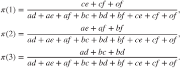
If ![]() is irreducible, then there exists a unique invariant law
is irreducible, then there exists a unique invariant law ![]() , given by
, given by
The chain with a finite number of states
Let ![]() . The above-mentioned method can be extended without any theoretical problem.
. The above-mentioned method can be extended without any theoretical problem.
The Euclidean division ![]() and
and ![]() yield that
yield that
If ![]() are the distinct roots of
are the distinct roots of ![]() and
and ![]() are their multiplicities, then
are their multiplicities, then
is a system of ![]() linearly independent equations for the
linearly independent equations for the ![]() unknowns
unknowns ![]() , which thus has a unique solution.
, which thus has a unique solution.
The enormous obstacle for the effective implementation of this method for computing ![]() is that we must compute the roots of
is that we must compute the roots of ![]() first. The main information we have is that
first. The main information we have is that ![]() is a root, and in general, computing the roots becomes a considerable problem as soon as
is a root, and in general, computing the roots becomes a considerable problem as soon as ![]() . Once the roots are found, solving the linear system and finding the invariant laws is a problem only when
. Once the roots are found, solving the linear system and finding the invariant laws is a problem only when ![]() is much larger.
is much larger.
This general method is simpler than finding the reduced Jordan form ![]() for
for ![]() , which also necessitates to find the roots of the characteristic polynomial
, which also necessitates to find the roots of the characteristic polynomial ![]() , and then solving a linear system to find the change-of-basis matrix
, and then solving a linear system to find the change-of-basis matrix ![]() and its inverse
and its inverse ![]() . Then,
. Then, ![]() , where
, where ![]() can be made explicit.
can be made explicit.
1.4 Detailed examples
We are going to describe in informal manner some problems concerning random evolutions, for which the answers will obviously depend on some data or parameters. We then will model these problems using Markov chains.
These models will be studied in detail all along our study of Markov chains, which they will help to illustrate.
In these descriptions, random variables and draws will be supposed to be independent if not stated otherwise.
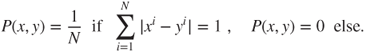
1.4.1 Random walk on a network
A particle evolves on a network ![]() , that is, on a discrete additive subgroup such as
, that is, on a discrete additive subgroup such as ![]() . From
. From ![]() in
in ![]() , it chooses to go to
, it chooses to go to ![]() in
in ![]() with probability
with probability ![]() , which satisfies
, which satisfies ![]() . This can be, for instance, a model for the evolution of an electron in a network of crystals.
. This can be, for instance, a model for the evolution of an electron in a network of crystals.
Some natural questions are the following:
- Does the particle escape to infinity?
- If yes, at what speed?
- With what probability does it reach a certain subset in finite time?
- What is the mean time for that?
1.4.1.1 Modeling
Let ![]() be a sequence of i.i.d. random variables such that
be a sequence of i.i.d. random variables such that ![]() , and
, and
Theorem 1.2.3 shows that ![]() is a Markov chain on
is a Markov chain on ![]() , with a transition matrix, which is spatially homogeneous, or invariant by translation, given by
, with a transition matrix, which is spatially homogeneous, or invariant by translation, given by
The matrix ![]() restricted to the network generated by all
restricted to the network generated by all ![]() such that
such that ![]() is irreducible. The constant measures are invariant, as
is irreducible. The constant measures are invariant, as
If ![]() , then the strong law of large numbers yields that
, then the strong law of large numbers yields that
and for ![]() the chain goes to infinity in the direction of
the chain goes to infinity in the direction of ![]() . The case
. The case ![]() is problematic, and if
is problematic, and if ![]() , then the central limit theorem shows that
, then the central limit theorem shows that ![]() converges in law to
converges in law to ![]() , which gives some hints to the long-time behavior of the chain.
, which gives some hints to the long-time behavior of the chain.
Nearest-neighbor random walk
For ![]() , this Markov chain is called a nearest-neighbor random walk when
, this Markov chain is called a nearest-neighbor random walk when ![]() for
for ![]() , and the symmetric nearest-neighbor random walk when
, and the symmetric nearest-neighbor random walk when ![]() for
for ![]() . These terminologies are used for other regular networks, such as the one in Figure 1.1.
. These terminologies are used for other regular networks, such as the one in Figure 1.1.
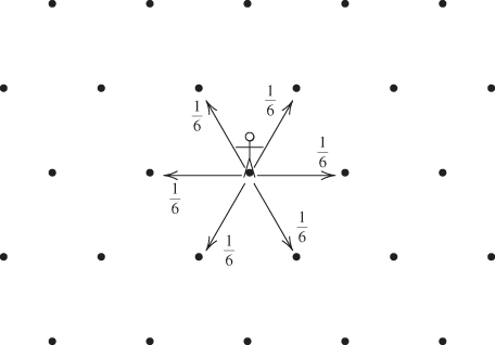
Figure 1.1 Symmetric nearest-neighbor random walk on regular planar triangular network.
1.4.2 Gambler's ruin
Two gamblers A and B play a game of head or tails. Gambler A starts with a fortune of ![]() units of money and Gambler B of
units of money and Gambler B of ![]() units. At each toss, each gambler makes a bet of
units. At each toss, each gambler makes a bet of ![]() unit, Gambler A wins with probability
unit, Gambler A wins with probability ![]() and loses with probability
and loses with probability ![]() , and the total of the bets is given to the winner; a gambler thus either wins or loses
, and the total of the bets is given to the winner; a gambler thus either wins or loses ![]() unit.
unit.
The game continues until one of the gamblers is ruined: he or she is left with a fortune of ![]() units, the global winner with a fortune of
units, the global winner with a fortune of ![]() units, and the game stops. This is illustrated in Figure 1.2.
units, and the game stops. This is illustrated in Figure 1.2.
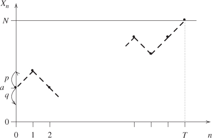
Figure 1.2 Gambler's ruin. Gambler A finishes the game at time  with a gain of
  units starting from a fortune of
  units. The successive states of his fortune are represented by the • and joined by dashes. The arrows on the vertical axis give his probabilities of winning or losing at each toss.
When ![]() , the game is said to be fair, else to be biased.
, the game is said to be fair, else to be biased.
As an example, Gambler A goes to a casino (Gambler B). He decides to gamble ![]() unit at each draw of red or black at roulette and to stop either after having won a total of
unit at each draw of red or black at roulette and to stop either after having won a total of ![]() units (what he or she would like to gain) or lost a total of
units (what he or she would like to gain) or lost a total of ![]() units (the maximal loss he or she allows himself).
units (the maximal loss he or she allows himself).
Owing to the ![]() and (most usually) the double
and (most usually) the double ![]() on the roulette, which are neither red nor black, the game is biased against him, and
on the roulette, which are neither red nor black, the game is biased against him, and ![]() is worth either
is worth either ![]() if there is no double
if there is no double ![]() or
or ![]() if there is one.
if there is one.
From a formal point of view, there is a symmetry in the game obtained by switching ![]() and
and ![]() simultaneously with
simultaneously with ![]() and
and ![]() . In practice, no casino allows a bias in favor of the gambler, nor even a fair game.
. In practice, no casino allows a bias in favor of the gambler, nor even a fair game.
A unilateral case will also be considered, in which ![]() and
and ![]() . In the casino example, this corresponds to a compulsive gambler, who will stop only when ruined. In all cases, the evolution of the gambler's fortune is given by a nearest-neighbor random walk on
. In the casino example, this corresponds to a compulsive gambler, who will stop only when ruined. In all cases, the evolution of the gambler's fortune is given by a nearest-neighbor random walk on ![]() , stopped when it hits a certain boundary.
, stopped when it hits a certain boundary.
Some natural questions are the following:
- What is the probability that Gambler A will be eventually ruined?
- Will the game eventually end ?
- If yes, what is the mean duration of the game?
- What is the law of the duration of the game (possibly infinite) ?
1.4.2.1 Stopped random walk
In all cases, the evolution of the gambler's fortune is given by a nearest-neighbor random walk on ![]() stopped when it hits a certain boundary.
stopped when it hits a certain boundary.
1.4.2.2 Modeling
The evolution of the fortune of Gambler A can be represented using a sequence ![]() of i.i.d. r.v. satisfying
of i.i.d. r.v. satisfying ![]() and
and ![]() by
by
where ![]() is its initial fortune
is its initial fortune ![]() , or more generally a r.v. with values in
, or more generally a r.v. with values in ![]() and independent of
and independent of ![]() . Gambler B's fortune at time
. Gambler B's fortune at time ![]() is
is ![]() .
.
Theorem 1.2.3 yields that ![]() is a Markov chain on
is a Markov chain on ![]() with matrix and graph given by
with matrix and graph given by
the other terms of ![]() being 0.
being 0.
The states ![]() and
and ![]() are absorbing, hence
are absorbing, hence ![]() is not irreducible. The invariant measures
is not irreducible. The invariant measures ![]() are of the form
are of the form ![]() if
if ![]() with
with ![]() and
and ![]() arbitrary, and uniqueness does not hold (uniqueness being understood as “up to proportionality”).
arbitrary, and uniqueness does not hold (uniqueness being understood as “up to proportionality”).
1.4.3 Branching process: evolution of a population
We study the successive generation of a population, constituted for instance of viruses in an organism, of infected people during an epidemic, or of neutrons during an atomic reaction.
The individuals of one generation disappear in the following, giving birth there each to ![]() descendants with probability
descendants with probability ![]() , with
, with ![]() . A classic subcase is that of a binary division:
. A classic subcase is that of a binary division: ![]() and
and ![]() .
.
The result of this random evolution mechanism is called a branching process. It is also called a Galton–Watson process; the initial study of Galton and Watson, preceded by a similar study of Bienaymé, bore on family names in Great Britain.
Some natural questions are the following:
- What is the law of the number of individuals in the
 th generation?
 - Will the population become extinct, almost surely (a.s.), and else with what probability?
- What is the long-time population behavior when it does not become extinct?
1.4.3.1 Modeling
We shall construct a Markov chain ![]() corresponding to the sizes (numbers of individuals) of the population along the generations.
corresponding to the sizes (numbers of individuals) of the population along the generations.
Let ![]() be i.i.d. r.v. such that
be i.i.d. r.v. such that ![]() for
for ![]() in
in ![]() . We assume that the
. We assume that the ![]() individuals of generation
individuals of generation ![]() are numbered
are numbered ![]() and that the
and that the ![]() th one yields
th one yields ![]() descendants in generation
descendants in generation ![]() , so that
, so that
(An empty sum being null by convention.)
Figure 1.3 illustrates this using the genealogical tree of a population, which gives the relationships between individuals in addition to the sizes of the generations, and explains the term “branching.”
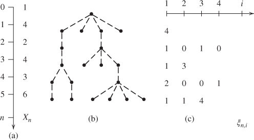
Figure 1.3 Branching process. (b) The genealogical tree for a population during six generations; • represent individuals and dashed lines their parental relations. (a) The vertical axis gives the numbers  of the generations, of which the sizes figure on its right. (c) The table underneath the horizontal axis gives the
  for
for  and
and  , of which the sum over
  yields
  .
.
The state space of ![]() is
is ![]() , and Theorem 1.2.3 applied to
, and Theorem 1.2.3 applied to ![]() yields that it is a Markov chain. The transition matrix is given by
yields that it is a Markov chain. The transition matrix is given by
and state ![]() is absorbing. The matrix is not practical to use under this form.
is absorbing. The matrix is not practical to use under this form.
It is much more practical to use generating functions. If
denotes the generating function of the reproduction law, the i.i.d. manner in which individuals reproduce yields that
For ![]() in
in ![]() , let
, let
denote the generating function of the size of generation ![]() . An elementary probabilistic computation yields that, for
. An elementary probabilistic computation yields that, for ![]() ,
,
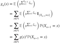
and hence that
We will later see how to obtain this result by Markov chain techniques and then how to exploit it.
1.4.4 Ehrenfest's Urn
A container (urn,…) is constituted of two communicating compartments and contains a large number of particles (such as gas molecules). These are initially distributed in the two compartments according to some law, and move around and can switch compartment.
Tatiana and Paul Ehrenfest proposed a statistical mechanics model for this phenomenon. It is a discrete time model, in which at each step a particle is chosen uniformly among all particles and changes compartment. See Figure 1.4.
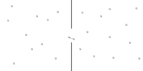
Figure 1.4 The Ehrenfest Urn. Shown at an instant when a particle transits from the right compartment to the left one. The choice of the particle that changes compartment at each step is uniform.
Some natural questions are the following:
- starting from an unbalanced distribution of particles between compartments, is the distribution of particles going to become more balanced in time?
- In what sense, with what uncertainty, at what rate?
- Is the distribution going to go through astonishing states, such as having all particles in a single compartment, and at what frequency?
1.4.4.1 Microscopic modeling
Let ![]() be the number of molecules, and let the compartments be numbered by
be the number of molecules, and let the compartments be numbered by ![]() and
and ![]() .
.
A microscopic description of the system at time ![]() is given by
is given by
where the ![]() th coordinate
th coordinate ![]() is the number of the compartment in which the
is the number of the compartment in which the ![]() th particle is located.
th particle is located.
Starting from a sequence ![]() of i.i.d. r.v. which are uniform on
of i.i.d. r.v. which are uniform on ![]() , and an initial r.v.
, and an initial r.v. ![]() independent of this sequence, we define recursively
independent of this sequence, we define recursively ![]() for
for ![]() by changing the coordinate of rank
by changing the coordinate of rank ![]() of
of ![]() . This random recursion is a faithful rendering of the particle dynamics.
. This random recursion is a faithful rendering of the particle dynamics.
Theorem 1.2.3 implies that ![]() is a Markov chain on
is a Markov chain on ![]() with matrix given by
with matrix given by
This is the symmetric nearest-neighbor random walk on the unit hypercube ![]() . This chain is irreducible.
. This chain is irreducible.
Invariant law
This chain has for unique invariant law the uniform law ![]() with density
with density ![]() .
.
As the typical magnitude of ![]() is comparable to the Avogadro number
is comparable to the Avogadro number ![]() , the number
, the number ![]() of configurations is enormously huge. Any computation, even for the invariant law, is of a combinatorial nature and will be most likely untractable.
of configurations is enormously huge. Any computation, even for the invariant law, is of a combinatorial nature and will be most likely untractable.
1.4.4.2 Reduced macroscopic description
According to statistical mechanics, we should take advantage of the symmetries of the system, in order to stop following individual particles and consider collective behaviors instead.
A reduced macroscopic description of the system is the number of particles in compartment ![]() at time
at time ![]() , given in terms of the microscopic description by
, given in terms of the microscopic description by
The information carried by ![]() being less than the information carried by
being less than the information carried by ![]() , it is not clear that
, it is not clear that ![]() is a Markov chain, but the symmetry of particle dynamics will allow to prove it.
is a Markov chain, but the symmetry of particle dynamics will allow to prove it.
For ![]() , let
, let ![]() be the permutation of
be the permutation of ![]() obtained by first placing in increasing order the
obtained by first placing in increasing order the ![]() such that
such that ![]() and then by increasing order the
and then by increasing order the ![]() such that
such that ![]() . Setting
. Setting
it holds that
For some deterministic ![]() and
and ![]() , using the random recursion for
, using the random recursion for ![]() ,
,
and hence, for all ![]() and
and ![]() ,
,
as ![]() is uniform and independent of
is uniform and independent of ![]() . Hence,
. Hence, ![]() is uniform on
is uniform on ![]() and independent of
and independent of ![]() . By a simple recursion, we conclude that the
. By a simple recursion, we conclude that the ![]() are i.i.d. r.v. which are uniform on
are i.i.d. r.v. which are uniform on ![]() and independent of
and independent of ![]() and hence of
and hence of ![]() .
.
Thus, Theorem 1.2.3 yields that ![]() is a Markov chain on
is a Markov chain on ![]() with matrix
with matrix ![]() and graph given by
and graph given by

all other terms of ![]() being zero. As
being zero. As ![]() is irreducible on
is irreducible on ![]() , it is clear that
, it is clear that ![]() is irreducible on
is irreducible on ![]() , and this can be readily checked.
, and this can be readily checked.
Invariant law
As the uniform law on ![]() , with density
, with density ![]() , is invariant for
, is invariant for ![]() , a simple combinatorial computation yields that the invariant law for
, a simple combinatorial computation yields that the invariant law for ![]() is binomial
is binomial ![]() , given by
, given by
This law distributes the particles uniformly in both compartments, and this is preserved by the random evolution.