Solutions for Chapter 2

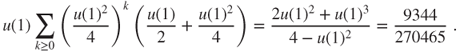
1. 2.1 Then, , , and .
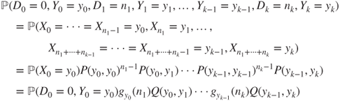
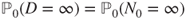
2. 2.2.a By definition of stopping times, and belong to . Thus, by definition of the -field ,
   
3. also belong to , and and are also stopping times. Moreover,
   
4. where , and can be written as so that . Hence, , and thus, is a stopping time.
5. 2.2.b If and , then
   
6. and hence . Applying this to and yields that . If , then
   
7. and hence, . Thus, .
8. 2.2.c Then, and and thus, , which is a -field, and thus, . Conversely, let . Then,
   
9. and thus, , and similarly , hence
   
10. We conclude that .
11. 2.3.a The matrix is Markovian as
    
12. Moreover,
    
13. 2.3.b As , the are stopping times. Moreover,
    
14. as
    
15. 2.3.c Let , , and . If , , , then
    

    or else the first and last terms in the previous equation are b03 zero and hence equal. Thus, is a Markov chain with the said transition matrix.

    Summation over yields that

    

    and thus, is a Markov chain with matrix . The Markov property yields that

    

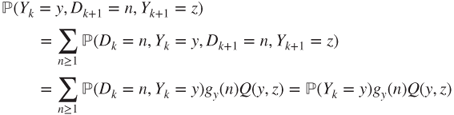
    and hence,

    

    Thus,

    
16. 2.3.d Then, . By definition of filtrations, can be written as and as . If , then can be written in terms of , i.e. that is, there exists a deterministic function such that . Hence,
    
17. so that is a stopping time for .
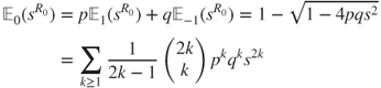
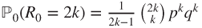
18. 2.4.a Then, . Actually, is the first hitting time of the diagonal by .
19. 2.4.b Then,
    

    and the first r.h.s. term can be expressed as the sum over of

    

    and the fact that also has matrix , , and the Markov property (Theorem 2.1.1) yields that this expression can be written as

    

    By summing all these terms, we find that

    

    and hence, has same law as .

    Thus,

    
20. 2.4.c All this is straightforward to check.
21. 2.4.d For , it holds that , and the Markov property (Theorem 2.1.1) yields that
    
22. and we conclude by iteration, considering that .
23. 2.4.e By assumption,
    
24. and we conclude by summing over and then over .
25. 2.4.f As and , we conclude by the previous results.
26. 2.5.a Let . We are interested in .

    By symmetry, , and the “one step forward” method (Theorem 2.2.2) yields that and and and and . Hence,

    

    and thus .

27. 2.5.b The visit consists in reaching module from module by one side, go times back and forth from module to module on that side, then either go to module by the other side or go to module by the same side, and then reach module from module by the other side, all this without visiting module .

    The Markov property (Theorem 2.1.3) and symmetry arguments yield that the probability of this event is

    
28. 2.5.c Let for . We are interested in .

    By symmetry, , and the “one step forward” method (Theorem 2.2.5) yields that and , , and , and . Hence,

    

    so that .

    We again find that , and by identification

    

    Moreover,

    

    and hence, by identification.

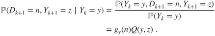
29. 2.6 We are interested in for and . Let .

    Then, by the “one step forward” method.

    This method also yields that (Theorem 2.2.5) and , , , , . Thus, and and then,

    

    and hence, , and finally,

    

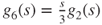
    Then, , the conditional generating function is given by , and a Taylor expansion at yields

    

    and thus, by identification, the conditional expectation is .

30. 2.7 If for , then . The “one step forward” method (Theorem 2.2.5) yields that and
    
31. so that
    
32. By identification,
    
33. Moreover, the Taylor expansion
    
34. yields that .
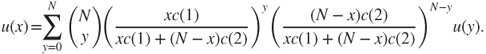
35. 2.8.a This equation writes, for ,
    
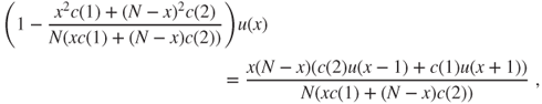
36. is of the form and has as a solution, hence the result. (The direct computation is simple.)
37. 2.8.b This is the same equation found in the Dirichlet problem in gambler's ruin when the gain probability at each toss for Gambler A is (see Section 2.3.1). We refer to that section for the computation of and .
38. 2.8.c Transitions are according to a binomial law. The equation is, for ,
    
39. If , then 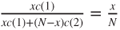and classically (total mass and expectation of a binomial law) for 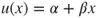, the r.h.s. of the equation takes the value 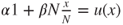, and hence, as for gambler's ruin, and .
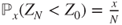40. 2.9.a The graph can be found in Section 3.1.3. Clearly, is irreducible.
41. 2.9.b If , then . For , a simple spatial translation allows to use the results in Section 2.3.2. For , it suffices to interchange and as well as and and use the previous result.
42. 2.9.c By the “one step forward” method, 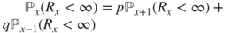and . Hence, the results follow from the previous ones.
43. 2.9.d The strong Markov property (Theorem 2.1.3) and the preceding results allow to compute . Moreover, .
44. 2.9.e If , then for all and the chain goes to infinity, a.s. More precisely, if , then as previously shown for , and thus . Similarly, if , then .
45. 2.9.f Then, and we conclude by a previous result.

    If a.s., then cannot hit , and hence does not have same law as . By contradiction, cannot be a stopping time, as then the strong Markov property would have applied.

46. 2.9.g Then,
    

    and previous results allow to conclude.

    If , then cannot reach a state greater than its initial value, and hence does not have same law as . By contradiction, cannot be a stopping time, as then the strong Markov property would have applied.

47. 2.9.h If , then 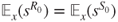, hence the result. The result for is obtained by symmetry.
48. 2.9.i The “one step forward” method yields that
    
49. in which we use the classic Taylor expansion provided at the end of Section 2.3.2. By identification, for .
50. 2.10.a We have for .
51. 2.10.b Straightforward, notably is clearly irreducible.
52. 2.10.c The “one step forward” method (Theorem 2.2.2) yields the equation. Its characteristic polynomial is 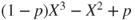, and its roots are and and . This yields the general solution, considering the case of multiple roots.
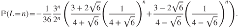
53. 2.10.d We have only two boundary conditions, whereas the space of general solutions is of dimension three, so we must use the minimality result in Theorem 2.(2.2 to find the solution of interest.
54. 2.10.e We use Theorem 2.(2.6 and seek the least solution with values in . We use the above-mentioned general solution for the associated linear equation, and a particular solution of the form when is a simple root and if it is a double.
55. 2.10.f We may use Theorem 2.2.5, but we do not have a trivial solution for the characteristic polynomial of degree three for the linear recursion.