
11
DEA‐DISCRIMINANT ANALYSIS
11.1 INTRODUCTION
This chapter discusses discriminant analysis (DA)1. DA2 is a classification method that can predict the group membership of a newly sampled observation. In the use of DA, a group of observations, whose memberships are already identified, are used for the estimation of weights (or parameters)3 of a discriminant function by some criterion such as minimization of misclassifications or maximization of correct classifications. A new sample is classified into one of several groups by the DA results.
In the last two decades, Sueyoshi (1999a, 2001b, 2004, 2005a, b, 2006), Sueyoshi and Kirihara (1998), Sueyoshi and Hwang (2004a), Sueyoshi and Goto (2009a,b,c, 2012c, 2013b)4 and Goto (2012) proposed a new type of non‐parametric DA approach that provides a set of weights of a linear discriminant function(s), consequently yielding an evaluation score(s) for determining group membership. The new non‐parametric DA is referred to as “DEA‐DA” because it maintains discriminant capabilities by incorporating the non‐parametric feature of DEA into DA. An important feature of DEA‐DA5 is that it can be considered as an extension of frontier analysis, using the L1‐regression analysis discussed in Chapter 3. Moreover, a series of research efforts has attempted to formulate DEA‐DA in the manner that they can handle a data set that contains zero and/or negative values. Thus, the development of DEA‐DA in this chapter is different from that of DEA discussed in previous chapters 6. See Chapters 26 and 27 that discuss how to handle zero and/or negative values in DEA environmental assessment.
The remainder of this chapter is organized as follows: Section 11.2 describes two mixed integer programming (MIP) formulations for DEA‐DA. Section 11.3 extends the proposed DEA‐DA approach to the classification of multiple groups. Methodological comparison by using illustrative data sets is documented in Section 11.4. Section 11.5 reorganizes the proposed approach from frontier analysis so that this chapter discusses an analytical linkage between DEA‐DA and DEA‐based frontier analysis. Concluding comments are summarized in Section 11.6.
11.2 TWO MIP APPROACHES FOR DEA‐DA
11.2.1 Standard MIP Approach
Consider a classification problem in which there are two groups (G1 and G2). Here, G1 is a set of observations in the first group above an estimated discriminant function and G2 is a set of observations in the second group below that estimated discriminant function. The sum of the two groups contains n observations ( j = 1,…, n). Each observation is characterized by m independent factors (i = 1,…, m), denoted by zij. Note that there is no distinction between inputs and outputs in DEA‐DA, as found in the previous chapters on DEA. The group membership of each observation should be known before the DA computation. The observation (zij) may consist of a data set that contains zero, positive and/or negative values.
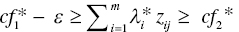
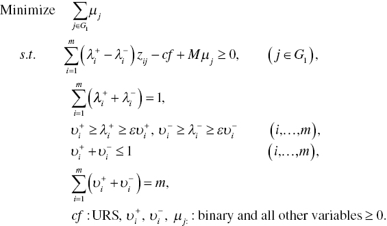
The single‐stage approach, often referred to as a “standard MIP approach,” is originally formulated as follows:
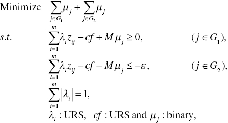
where M is a given large number (e.g., 10000) and ε is a given small number (e.g., 1). Both should be prescribed before the computation of Model (11.1). The objective function minimizes the total number of incorrectly classified observations by counting a binary variable (μj). The binary variable (0 or 1) expresses correct or incorrect classification. A discriminant score for cutting‐off between two groups is expressed by cf ( j ![]() G1) and cf‐ε ( j
G1) and cf‐ε ( j ![]() G2), respectively. The small number (ε) is incorporated into Model (11.1) in order to avoid a case where an observation(s) exists on an estimated discriminant function. Thus, the small number is for perfect classification. Furthermore, a weight estimate regarding the i‐th factor is expressed by λi. All the observations (zij for all i and j) are connected by a weighted linear combination, or
G2), respectively. The small number (ε) is incorporated into Model (11.1) in order to avoid a case where an observation(s) exists on an estimated discriminant function. Thus, the small number is for perfect classification. Furthermore, a weight estimate regarding the i‐th factor is expressed by λi. All the observations (zij for all i and j) are connected by a weighted linear combination, or ![]() , that consists of a discriminant function. The weights on factors are restricted in such a manner that the sum of absolute values of λi (i = 1,..., m) is unity in Model (11.1). The treatment is because we need to deal with zero and/or negative values in an observed data set. It is easily thought that λi is a weight on each factor, not each observation (i.e., DMU), as found in a conventional use of DA. The weight simply expresses the importance of each factor in terms of estimating a discriminant function. The importance among weight estimates is specified by a percentage expression.
, that consists of a discriminant function. The weights on factors are restricted in such a manner that the sum of absolute values of λi (i = 1,..., m) is unity in Model (11.1). The treatment is because we need to deal with zero and/or negative values in an observed data set. It is easily thought that λi is a weight on each factor, not each observation (i.e., DMU), as found in a conventional use of DA. The weight simply expresses the importance of each factor in terms of estimating a discriminant function. The importance among weight estimates is specified by a percentage expression.
It is possible for us to formulate Model (11.1) by maximizing the number of correct classifications. Both incorrect minimization and correct maximization does not produce a major difference between them. Because of different MIP formulations and different computations (i.e., minimization or maximization), the two approaches may produce different but similar results in terms of their classification capabilities.
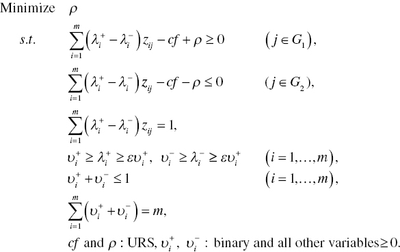
In examining Model (11.1), we understand that it is difficult for us to directly solve the model because ![]() =1 is incorporated in the formulation. Hence, Model (11.1) needs to be reformulated by separating each weight λi(
=1 is incorporated in the formulation. Hence, Model (11.1) needs to be reformulated by separating each weight λi(![]() ) for i = 1,…, m. Here,
) for i = 1,…, m. Here, ![]() and
and ![]() indicate the positive and negative parts of the i‐th weight, respectively.
indicate the positive and negative parts of the i‐th weight, respectively.
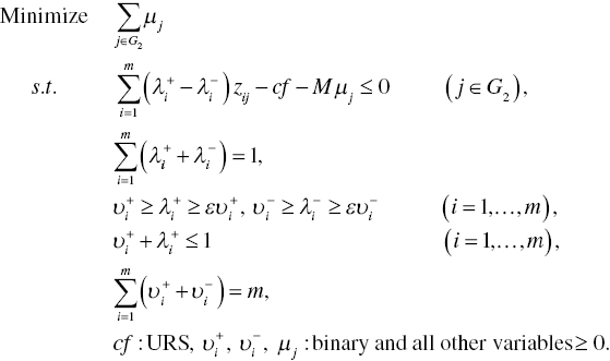
Following the research effort of Sueyoshi (2006), this chapter reformulates Model (11.1) as follows:
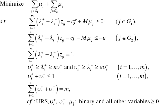
In Model (11.2), binary variables (![]() and
and ![]() for i = 1,…, m) are incorporated in the formulation. The first two groups of constraints in Model (11.2) are originated from those of Model (11.1). The third constraint expresses |λi| by
for i = 1,…, m) are incorporated in the formulation. The first two groups of constraints in Model (11.2) are originated from those of Model (11.1). The third constraint expresses |λi| by ![]() for i = 1,…, m. The third one is often referred to as “normalization” in the DA community. The fourth group of constraints indicate the upper and lower bounds of
for i = 1,…, m. The third one is often referred to as “normalization” in the DA community. The fourth group of constraints indicate the upper and lower bounds of ![]() and those of
and those of ![]() , respectively. The fifth group of constraints implies that the sum of binary variables (
, respectively. The fifth group of constraints implies that the sum of binary variables (![]() and
and ![]() for all i) is less than or equal to unity. The restriction avoids a simultaneous occurrence of
for all i) is less than or equal to unity. The restriction avoids a simultaneous occurrence of ![]() > 0 and
> 0 and ![]() > 0. The last constraints are incorporated into Model (11.2) in order to utilize all weights (so, being a full model for a discriminant function).
> 0. The last constraints are incorporated into Model (11.2) in order to utilize all weights (so, being a full model for a discriminant function).
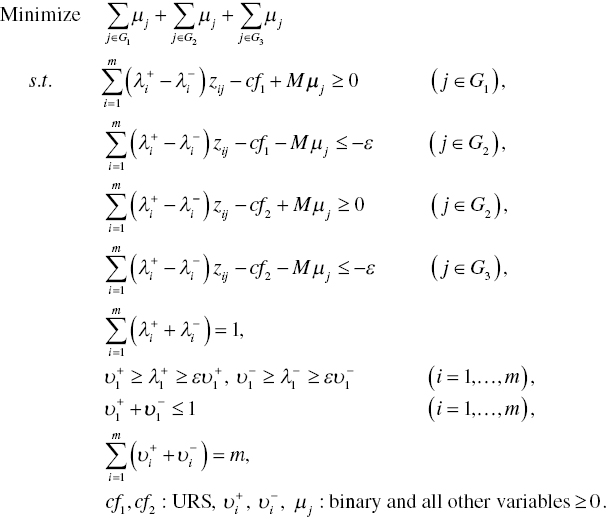
All observations, or Zj = (z1j, …, zmj)Tr for all j, are classified by the following rule:
- If
 cf *, then the j‐th observation belongs to G1, and
 - If
 ≤
≤  , then the j‐th observation belongs to G2.
Here, ![]() (i = 1,…, m) and cf * are obtained from the optimality of Model (11.2). The classification of a new sample, or Zk = (z1k, …, zmk)Tr for the specific k, is determined by the same rule by replacing the subscript j by k in the classification rule.
(i = 1,…, m) and cf * are obtained from the optimality of Model (11.2). The classification of a new sample, or Zk = (z1k, …, zmk)Tr for the specific k, is determined by the same rule by replacing the subscript j by k in the classification rule.
A methodological strength of the standard MIP approach is that we can utilize a single classification (![]() for all i = 1,…, m and cf *). A drawback of the approach is that the computation effort on Model (11.2) is more complex and more tedious (i.e., more time‐consuming) than that of the two‐stage MIP approach, discussed in Section 11.2.2. The computational concern seems inconsistent with our expectation. The rationale concerning why the computational efficiency occurs in the two‐stage MIP approach will be discussed in the next subsection.
for all i = 1,…, m and cf *). A drawback of the approach is that the computation effort on Model (11.2) is more complex and more tedious (i.e., more time‐consuming) than that of the two‐stage MIP approach, discussed in Section 11.2.2. The computational concern seems inconsistent with our expectation. The rationale concerning why the computational efficiency occurs in the two‐stage MIP approach will be discussed in the next subsection.
Although the standard MIP approach is more time‐consuming than the two‐stage MIP approach in solving various DA problems, the former has an analytical benefit that should be noted here. That is, it is possible for us to reformulate Model (11.2) by linear programing which minimizes the total amount of slacks for expressing distances between observations of independent factors and an estimated discriminant function. It is trivial that a linear programming formulation is more efficient than the proposed MIP formulation, or Model (11.2). This chapter, along with Chapter 25, does not describe the linear programming formulation, because the performance of DA is usually evaluated by a classification rate, as documented in this chapter. Of course, we clearly understand that if we discuss frontier analysis, a linear programming formulation is sufficient enough to develop an efficiency frontier for measuring a degree of OE. See Chapter 3 on frontier analysis.
11.2.2 Two‐stage MIP Approach
It is widely known that the main source of misclassification in DA is due to the existence of an overlap between two groups in a data set. This type of problem does not occur in DEA. If we expect to increase the number of observations classified correctly, then DA approaches must consider how to handle an existence of such an overlap. If there is no overlap, most DA approaches can produce a perfect, or almost perfect, classification. However, if there is an overlap in the observations, an additional computation process is usually necessary to deal with this overlap. Thus, it is expected at the initial stage of DA that there is a tradeoff between computational effort (time) and level of classification capability.
In this chapter, a two‐stage approach is proposed to handle such an overlap and thus increase the classification capability of DA. Surprisingly, this two‐stage approach may decrease the computational burden regarding DA, depending upon the size of the overlap. The proposed computation process of the two‐stage approach consists of classification and overlap identification, along with handling the overlap.
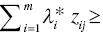
The first stage of the two‐stage approach, discussed by Sueyoshi (2006), is formulated as follows:
Stage 1: Classification and Overlap Identification (COI):
In Model (11.3), the unrestricted variable “ρ” indicates the absolute distance between the discriminant score and a discriminant function.
Let ![]() (=
(=![]() ), cf* and ρ * be the optimal solution of the first stage (COI), or Model (11.3). On the optimality of Model (11.3), all observations on independent factors, or
), cf* and ρ * be the optimal solution of the first stage (COI), or Model (11.3). On the optimality of Model (11.3), all observations on independent factors, or ![]() , for j = 1,..., n are classified by the following rule:
, for j = 1,..., n are classified by the following rule:
- If
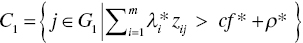
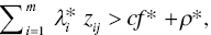 then the j‐th observation belongs to G1 (= C1),
 - If
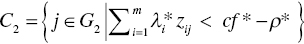
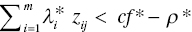 , then the observation belongs to G2 (= C2) and
 - If
 , then the observation belongs to an overlap.
Based upon the classification rule, the original sample data set (G) is classified into the following four subsets (![]() ):
):
 ,
, ,
, and
and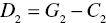 .
.
In the classification, C1 and C2 indicate a clearly above group and a clearly below group, respectively. Here, C1 is a partial group of G1 which are clearly above the estimated discriminant function in Stage 1 and C2 is a partial group of G2 which are clearly below the estimated discriminant function in Stage 1. The remaining two groups (![]() ) belong to the overlap in which D1 is a part of G1 and D2 is a part of G2. A new sample (Zk) is also classified by the above rules by replacing subscript j by subscript k.
) belong to the overlap in which D1 is a part of G1 and D2 is a part of G2. A new sample (Zk) is also classified by the above rules by replacing subscript j by subscript k.
Stage 2: Handling Overlap (HO):
The existence of an overlap is identified by ![]() at the first stage for overlap identification. In contrast,
at the first stage for overlap identification. In contrast, ![]() indicates no overlap between two groups. In the former case when the overlap is found between them, the second stage needs to reclassify all the observations, belonging to the overlap (
indicates no overlap between two groups. In the former case when the overlap is found between them, the second stage needs to reclassify all the observations, belonging to the overlap (![]() ), because the group membership of these observations is still unknown and not yet determined. Mathematically, the second (HO) stage is formulated as follows:
), because the group membership of these observations is still unknown and not yet determined. Mathematically, the second (HO) stage is formulated as follows:
In Model (11.4), the binary variable (μj) counts the number of observations classified incorrectly. These observations to be examined at the second stage are reduced from ![]() to
to ![]() as a result of the first stage. If the number of observations belonging to
as a result of the first stage. If the number of observations belonging to ![]() is larger than m (the number of weights to be estimated), then
is larger than m (the number of weights to be estimated), then ![]() = m is used in Model (11.4). However, if the number is less than m, then
= m is used in Model (11.4). However, if the number is less than m, then ![]() is used in Model (11.4) where the number “p” (< m) indicates a prescribed number in such a manner that p is less than or equal to the number of observations in
is used in Model (11.4) where the number “p” (< m) indicates a prescribed number in such a manner that p is less than or equal to the number of observations in ![]() . Thus, the degree of freedom needs to be considered for the selection of p. In reality, prior information is necessary for the selection of p.
. Thus, the degree of freedom needs to be considered for the selection of p. In reality, prior information is necessary for the selection of p.
Observations belonging to the overlap (D1![]() D2) are classified at the second (HO) stage by the following rule:
D2) are classified at the second (HO) stage by the following rule:
- If
 , then the j‐th observation in the overlap belongs to G1 and
 - If
 then the j‐th observation belongs to G2.
A new sample (Zk) is also classified by the above rule by replacing the subscript (j) by the one (k).
Figures 11.1 to 11.4 visually describe the classification processes of the two‐stage approach. For our visual convenience, Figure 11.1 has coordinates for z1 and z2, the two factors which depict observations belonging to two groups G1 and G2. Stage 1 is used to identify an occurrence of an overlap between two groups by two lines. Thus, Stage 1 classifies all observations into these three groups as follows: a part of G1, a part of G2 and an overlap group. In the classification, the clearly above group (C1) is part of G1 and the clearly below group (C2) is part of G2. See Figure 11.3 for a visual description of C1 and C2. The remaining group belongs to the overlap. Stage 1 cannot classify observations belonging to the overlap.
FIGURE 11.1 Classification and overlap identification at Stage 1

FIGURE 11.2 Overlap identification at Stage 1
FIGURE 11.3 Classification at Stage 1
FIGURE 11.4 Final classification at Stage 2
Figure 11.2 visually describes how Stage 1 determines the size of an overlap between two groups by using a distance measure (ρ). All the observations are classified into these three groups: C1 (clearly above), C2 (clearly below) and an overlap between them, as depicted in Figure 11.3. The distance measure (ρ) in Figure 11.2, which is unrestricted in the sign, has an important role in identifying the overlap size. That is, Stage 1 determines the lower bound of G1 by subtracting ρ from an estimated discriminant function and it determines the upper bound of G2 by adding ρ to an estimated discriminant function. The minimization of ρ in Model (11.3), which is visually specified in Figure 11.2, determines the size of the overlap located between the upper and lower bounds of the two groups.
Figure 11.3 depicts the classification of three groups. At the end of Stage 1, all the observations are separated into three groups: C1 (clearly above), C2 (clearly below) and an overlap that contains observations that are further separated into two subgroups (D1 and D2) at Stage 2.
Figure 11.4 visually describes the function of Stage 2 that separates observations belonging to the overlap into D1 and D2. D1 is the group of observations classified above the discriminant function and D2 is the group of observations classified below the discriminant function at the second stage. Thus, the group classification from G1 and G2 to C1, C2, D1 and D2 indicates the end of Stage 2.
Altman’s Z score: Following the work of Altman (1968, 1984), the performance of the j‐th DMU is measured by a score ![]() where
where ![]() is the i‐th weight estimate of a discriminant function. DEA‐DA cannot directly compute the Altman’s Z (AZ) score because the two‐stage approach produces two discriminant functions (so, double standards) for group classification. Hence, it is necessary for us to adjust the computation process to measure the AZ score.
is the i‐th weight estimate of a discriminant function. DEA‐DA cannot directly compute the Altman’s Z (AZ) score because the two‐stage approach produces two discriminant functions (so, double standards) for group classification. Hence, it is necessary for us to adjust the computation process to measure the AZ score.
To adjust the problem of double standards, this chapter returns to the proposed approach in which the first stage estimates a discriminant function ![]() and the second stage estimates a discriminant function
and the second stage estimates a discriminant function ![]() . The AZ score for the j‐th DMU ( j = 1,…, n) is defined as follows:
. The AZ score for the j‐th DMU ( j = 1,…, n) is defined as follows:

This chapter refers to Equation (11.5) as “Altman’s Z score,” or simply “AZ score.” Exactly speaking, the equation is slightly different from the equation for the original AZ score proposed by Altman (1968). However, this chapter uses the term to honor his research work.
The proposed AZ score consists of weight estimates that are adjusted by the number of observations used in the first and second stages of DEA‐DA. The adjustment is due to the computational process of DEA‐DA in which the first stage (for overlap identification) estimates weights of a discriminant function by using all the observations. The total sample size is “n” for the first stage. Meanwhile, the second stage utilizes only observations in the overlap. The sample size used in the second stage is #(overlap). Thus, this chapter combines two groups of weight estimates measured by DEA‐DA into a single set of weight estimates in order to compute the AZ score. Using the AZ score, DEA‐DA can determine the financial performance of each DMU. See Chapter 25 on the selection of common multipliers.
11.2.3 Differences between Two MIP Approaches
Before extending DEA‐DA into the classification of multiple groups, the following five comments are important for understanding the two MIP versions:
- First, the selection of M and ε influences the weight estimates (
 and cf *). Different selections may often produce different weight estimates. That is a drawback of the MIP versions of DEA‐DA. Thus, DEA‐DA may suffer from a methodological bias.
 - Second, mathematical programming approaches for DA do not attain methodological practicality at the level of statistical and econometric approaches, because there is no user‐friendly computer software to solve various DA problems. Moreover, statistical tests are not available to us, because asymptotic theory is not yet developed to the level of these conventional (statistical and econometrics) approaches.
- Third, the two‐stage MIP approach is effective only when many observations belong to an overlap. If the number of observations in the overlap is small, the performance of the standard MIP approach is similar to that of the two‐stage MIP approach in terms of classification performance.
- Fourth, the standard MIP approach may be practical in persuading corporate leaders and policy makers, because it produces a single separation function. A problem of the standard MIP approach is that it is more time‐consuming than the two‐stage MIP approach. The rationale on why the latter approach is more efficient than the former in terms of their computational times is because of the analytical structure of the two‐stage approach. That is, the number of binary variables at the first stage is much lower than that of the second stage. The second stage is similar to the standard approach in their analytical structures. A difference between the two is that the second stage has binary variables used to count the number of incorrectly classified observations in
 . The number is less than that of observations
  in the standard approach under
 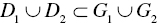 . Thus, the two‐stage approach is computationally more efficient than the standard approach. The former approach can handle much larger data sets than the latter approach.
 - Finally, although this chapter does not discuss it in detail, all DA research work must examine whether the sign of each weight is consistent with our prior information, such as previous experience and theoretical requirement. For example, when non‐default (G1) and default (G2) firms are separated by several financial factors (e.g., profit and return on equity; ROE), the sign of profit is expected to be positive. However, it may be negative due to some structural difficulty in a data set (e.g., multi‐collinearity). In that case, it is necessary for us to incorporate an additional side constraint(s), representing prior information, into the proposed DA formulations. See Sueyoshi and Kirihara (1998) for a detailed discussion on how to incorporate such prior information into DEA‐DA.
11.2.4 Differences between DEA and DEA‐DA
Table 11.1 compares DEA and DEA‐DA to summarize their differences. It is clearly identified that both DEA and DEA‐DA originate from GP, as discussed in Chapter 3. In their conventional uses, however, DEA is used for performance assessment and DEA‐DA is used for group classification.
TABLE 11.1 Differences between DEA and DEA‐DA
| Analytical features | DEA | DEA‐DA |
| Input and output classification and group classification |
|
|
| Non‐parametric | The j‐th weight estimate (multiplier) obtained by DEA indicates the importance of the j‐th observation or DMU in determining an efficiency frontier of the specific observation. | The i‐th weight estimate obtained by DEA‐DA indicates the importance of the i‐th factor variable for comprising a discriminant function to separate between the two groups. |
| Firm‐specific weights vs group‐wide common weights | The result of DEA is DMU‐specific so that the efficiency measure depends upon each DMU. | The result of DEA‐DA is group‐widely applicable because it provides “common weights” for all observations. |
| Distribution‐free | DEA does not have any assumption on how all observations locate below an efficiency frontier. | DEA‐DA does not need any assumption on a group distribution above and below a discriminant function. |
| Rank‐sum tests | No conventional statistical tests are available. Rank‐sum tests are available for DEA. | No conventional statistical tests are available. Rank‐sum tests are available for DEA‐DA. |
| Data imbalance | The data imbalance in DEA implies that a large input or output dominates the others. DEA can solve the problem of data imbalance by adjusting all inputs and outputs by these averages. | The data imbalance in DEA‐DA implies different sample sizes between two groups. DEA‐DA can deal with the problem of date imbalance by putting more weight on one of two groups. |
| Multiple solutions and multiple criteria | Multiple solutions may occur on DEA results. Efficiency of a DMU is determined by comparing its performance with an efficiency frontier. Thus, DEA consists of a single criterion. | An occurrence of multiple solutions in MIP approaches for DEA‐DA is not important. The standard approach has a single criterion for group classification, but the two‐stage approach has double standards for group classification. |
| Optimality | Since DEA is solved by linear programming, it can guarantee optimality. An exception is the Russell measure. | Since DEA‐DA is solved by MIP, it cannot guarantee optimality. |
11.3 CLASSIFYING MULTIPLE GROUPS
A shortcoming of the two MIP approaches (standard and two‐stage) is that they cannot handle the classification of more than two groups. To extend them to deal with more than two groups, this chapter considers the classification of three groups by using the standard MIP approach. Then, the formulation is further restructured into the classification of q groups (![]() 1,…, q).
1,…, q).
The classification of three groups can be formulated by slightly modifying the model in Equation (11.2) as follows:
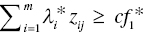
The modification of the above formulation is that it incorporates two discriminant scores (cf1 and cf2) in the model in Equation (11.6). The first discriminant score (cf1) for a cut‐off is used to separate between G1 and G2. The second one (cf2) is for the classification between G2 and G3.
All observations ![]() for j = 1,…, n, are classified as follows:
for j = 1,…, n, are classified as follows:
- If
 , then the j‐th observation belongs to G1,
 - If
 , then the observation belongs to G2 and
 - If
 , then the observation belongs to G3.
A newly sampled k‐th observation, ![]() , is classified by the above rule by changing the subscript (j) by the one (k).
, is classified by the above rule by changing the subscript (j) by the one (k).
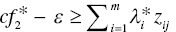
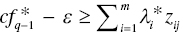
More Than Three Groups: The model in Equation (11.6) is further reformulated for classification of more than three groups. The following formulation provides the classification of multiple groups (![]() ):
):
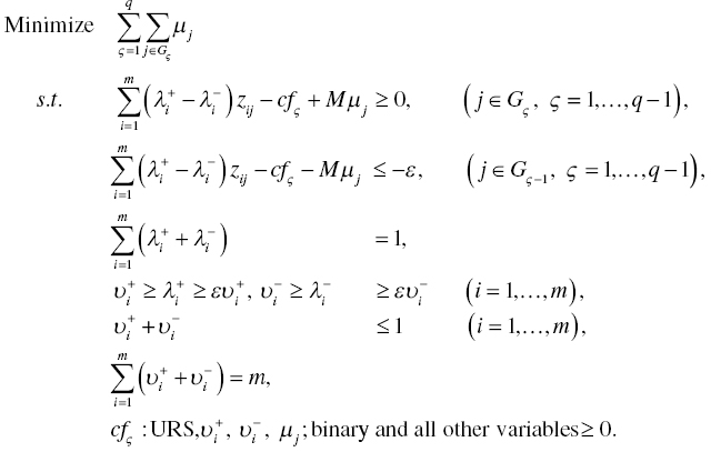
Here, Gς is a set of observations in the ς‐th group (for ς = 1,…, q–1), In the above case, multiple groups are separated by ![]() (
(![]() 1,…, q–1) and
1,…, q–1) and ![]() (i = 1,…, m), all of which are obtained from the optimality of the model in Equation (11.7).
(i = 1,…, m), all of which are obtained from the optimality of the model in Equation (11.7).
All observations ![]() for j = 1,…, n are classified as follows:
for j = 1,…, n are classified as follows:
- If
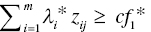 , then the observation belongs to G1,
 - If
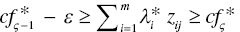 , then the observation belongs to Gς (ς = 2,…, q–1) and
 - If
 , then the observation belongs to Gq.
A newly sampled observation, or ![]() , is classified by the above rule by changing the subscript (j) by the one (k).
, is classified by the above rule by changing the subscript (j) by the one (k).
At the end of this subsection, the following three comments are necessary for using Model (11.7):
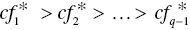
- First, a unique feature of Model (11.7) is that it produces q–1 different discriminant scores (
 to
to  ) in order to classify q groups. Furthermore, it maintains the same weight scores (
 , i = 1,…, m). Figure 11.5 visually describes the classification of multiple groups.
 - Second, when solving Model (11.7),
 is required on optimality. If such a requirement is not satisfied on the optimality, then additional side constraints:
  ,
,  ,…, and
 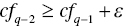 must be incorporated into Model (11.7). The additional capability is due to methodological flexibility of the MIP‐based approach.
 - Finally, the proposed MIP approach can solve only a specific type of multiple group classification, where the “specific” implies that a whole data set can be arranged in a particular ordering, as depicted in Figure 11.5. In other words, the particular ordering data implies the one that is classified into multiple groups by several separation functions whose slopes (i.e., weights) are same but having different intercepts (i.e., classification scores). If a date set does not have such a special ordering structure, Model (11.7) may produce an “infeasible” solution or a low classification rate. Thus, Model (11.7) has a limited capability for group classification.
FIGURE 11.5 Classification of multiple groups
(a) Source: Sueyoshi (2006).
(b) This type of multiple group classification by DEA‐DA has a limited classification capability because it produces same cutting off hyperplanes except an intercept. There is a possibility that DEA‐DA produces an infeasible solution when such hyperplanes cannot separate multiple groups
11.4 ILLUSTRATIVE EXAMPLES
11.4.1 First Example
This chapter uses two illustrative data sets to document the discriminant capabilities of the proposed DEA‐DA approaches. The first data set, listed in Table 11.2, contains 31 observations which are separated into two groups (G1: the first 20 observations and G2: the remaining second observations). Each observation is characterized by four factors.
TABLE 11.2 Illustrative data set and hit rates
(a) Source: Sueyoshi (2006).
| Observation (j) | Factor 1 | Factor 2 | Factor 3 | Factor 4 |
| 1 | 0.03 | 3.00 | 2.40 | 9.20 |
| 2 | 2.13 | 2.00 | 2.00 | 0.60 |
| 3 | 8.48 | 2.50 | 2.20 | 1.50 |
| 4 | 0.76 | 1.10 | 0.90 | 3.20 |
| 5 | 0.05 | 2.10 | 2.00 | 5.40 |
| 6 | 1.65 | 1.30 | 0.90 | 5.60 |
| 7 | 1.09 | 0.80 | 0.30 | 11.00 |
| 8 | 0.08 | 3.20 | 2.90 | 9.40 |
| 9 | 0.10 | 1.20 | 0.80 | 8.50 |
| 10 | 0.91 | 0.90 | 0.30 | 15.80 |
| 11 | 1.25 | 0.80 | 0.20 | 23.60 |
| 12 | 1.23 | 0.80 | 0.50 | 7.50 |
| 13 | 0.06 | 1.60 | 0.80 | 51.80 |
| 14 | 2.10 | 0.90 | 0.10 | 77.80 |
| 15 | 0.29 | 1.10 | 0.70 | 9.00 |
| 16 | 0.93 | 1.00 | 0.50 | 13.40 |
| 17 | 0.16 | 1.40 | 1.10 | 5.70 |
| 18 | 0.10 | 1.80 | 1.20 | 6.70 |
| 19 | 0.22 | 1.30 | 0.90 | 10.70 |
| 20 | 0.63 | 1.40 | 0.90 | 6.70 |
| 21 | 5.40 | 1.04 | 0.43 | 4.33 |
| 22 | 1.69 | 2.27 | 0.98 | 5.18 |
| 23 | 0.87 | 2.20 | 1.11 | 7.67 |
| 24 | 0.74 | 0.58 | 0.45 | 6.08 |
| 25 | 2.71 | 1.46 | 1.23 | 3.25 |
| 26 | 2.60 | 0.43 | 0.35 | 8.18 |
| 27 | 0.00 | 0.09 | 0.04 | 13.46 |
| 28 | 0.38 | 1.47 | 1.30 | 4.81 |
| 29 | 0.20 | 1.61 | 0.16 | 450.56 |
| 30 | 51.89 | 0.37 | 0.14 | 7.63 |
| 31 | 1.35 | 0.92 | 0.42 | 16.60 |
| Method | Hit rate (%) | |||
| Apparent | LOO | |||
| Standard MIP approach | 80.65 | 77.42 | ||
| Two‐stage MIP approach | 90.32 | 83.33 | ||
| Logit | 70.97 | 61.29 | ||
| Probit | 70.97 | 61.29 | ||
| Fisher’s linear DA | 67.70 | 51.60 | ||
| Smith’s quadratic DA | 80.60 | 67.70 | ||
The bottom of Table 11.2 summarizes two hit rates (apparent and leave one out: LOO) for six different DA methods. Here, “apparent” indicates the number of correctly classified observations in a training sample. In measuring the apparent of the first data set, all 31 observations become the training sample. In contrast, the LOO measurement drops each observation from the training sample and then applies a DA method to the remaining observations. LOO examines whether the omitted observation is correctly classified. Thus, the LOO measurement needs to be repeated until all the observations are examined.
Figure 11.6 depicts such a computation process to measure apparent and LOO. In the figure, the apparent measurement uses the whole data set as both a training sample set and a validation sample set. Meanwhile, the LOO measurement uses a single observation omitted from the whole data set as a test sample. The remaining data set is used as a training sample set.
FIGURE 11.6 Structure of performance measurement
(a) Source: Sueyoshi (2006)
As summarized in Table 11.2, the two‐stage MIP approach is the best performer in the apparent and LOO measurements (90.32 and 83.33%, respectively). Two econometric (logit and probit) approaches and Fisher’s linear DA perform insufficiently because the data set does not satisfy the underlying assumptions that are necessary for applying those DA methods. In contrast, a shortcoming of the MIP approaches is that they need computational times which are much longer than those of the other DA methods.
11.4.2 Second Example
The second data set, originally obtained from Sueyoshi (2001b, pp. 337–338), is related to Japanese banks that contains 100 observations. All the observations in the data set are listed by their corporate ranks. Therefore, G1 contains 50 banks ranked from the first to the 50th. Meanwhile, G2 contains the remaining 50 banks ranked from the 51st to the 100th. This data set has been extensively used by many studies on DA.
Data Accessibility: The data set is documented in Sueyoshi (2006).
In this chapter, the whole data set is used to apply four different grouping cases (two, three, four and five groups). To make each group, all 100 observations are classified by these ranks. For example, in the case of four groups, G1 consists of observations whose ranks are from the first to the 25th. G2 is a set of observations whose ranks are from the 26th to the 50th. Similarly, G3 and G4 are selected from the 51st to the 75th and the 76th to the 100th, respectively. Table 11.3 summarizes the weight estimates of Model (11.7) and two hit rates, all of which are obtained from Model (11.7) applied to the four different grouping cases.
TABLE 11.3 Weight estimates and hit rates (multiple classifications)
(a) Source: Sueyoshi (2006).
| Weight estimates | Multiple classification model | ||||
| Two group classification | Three group classification | Four group classification | Five group classification | ||
| λ1* | –0.03300 | –0.11556 | 0.20921 | 0.02930 | |
| λ2* | 0.03928 | 0.02861 | 0.01884 | 0.03663 | |
| λ3* | –0.03677 | –0.03153 | –0.04001 | –0.03241 | |
| λ4* | 0.83991 | 0.76601 | 0.68171 | 0.85212 | |
| λ5* | –0.04369 | –0.05120 | –0.02948 | –0.04316 | |
| λ6* | 0.00260 | 0.00616 | 0.00574 | 0.00488 | |
| λ7* | –0.00475 | –0.00094 | –0.01502 | –0.00149 | |
| cf1* | –1.76496 | –1.25426 | –1.80618 | –0.95670 | |
| cf2* | — | –1.44013 | –2.06284 | –1.17478 | |
| cf3* | — | — | –2.21214 | –1.33047 | |
| cf4* | — | — | — | –1.48890 | |
| Hit rate (%) | Apparent | 96 | 95 | 97 | 94 |
| LOO | 90 | 90 | 87 | 87 | |
11.5 FRONTIER ANALYSIS
It is possible for us to apply DEA‐DA for frontier analysis, as found in the L1 regression analysis of Chapter 3. See Chapter 25, as well. Since no research has explored that research issue, this chapter describes the analytical link between DEA‐DA and frontier analysis.
In applying DEA‐DA to frontier analysis, we can easily imagine two types of frontiers. One type is that all observations belong to G1, but G2 is empty. An estimated frontier function locates below all observations. The first case is formulated as follows:
The other case, where the frontier function locates above all observations, is formulated as follows:
Models (11.8) and (11.9) drop the small number (ε) from the right‐hand side because frontier analysis accepts that a few observations exist on the frontier. Of course, the small number (ε) in the two models can be used to maintain positive weights.
Applicability: Chapter 25 discusses how to apply the proposed DEA‐DA to the performance assessment of Japanese energy utility firms. Hence, this chapter does not document the applicability.
11.6 SUMMARY
This chapter discussed two MIP approaches for DEA‐DA and compared them with other DA models (e.g., Fisher, Smith, logit and probit), all of which were extensively used in conventional DA on statistics and econometrics. In comparison with these DA methods, this chapter confirmed that the MIP approaches for DEA‐DA performed at least as well as the other well known DA methods. Moreover, the standard MIP approach was extendable into the classification of multiple (more than two) groups in the data set, as depicted in Figure 11.5, along with a comment that such an extension has a limited classification capability.
It is true that there is no perfect methodology for DA. Any DA method, including the proposed two types of MIP approaches, has methodological strengths and shortcomings. The methodological drawbacks of the proposed MIP approaches are summarized by the following three concerns. First, the MIP approaches need asymptotic theory, based upon which we can derive statistical tests on DA. The statistical and econometric approaches can provide us with various statistical tests incorporated in prevalent computer software tools. The software, including such traditional approaches, is usually inexpensive. In many cases, users can freely access such DA methods. The availability of user‐friendly software including many statistical tests really enhances the practicality of the proposed MIP approaches. Second, a special computer algorithm must be developed for the proposed MIP approaches. The computational time of the proposed MIP approaches should be more drastically reduced at the level of statistical and econometric DA approaches. The methodological shortcoming is because the MIP formulations usually need a long computational time and some effort. In particular, the single‐stage approach is much more time‐consuming than the two‐stage approach. Finally, the selection of M and ε influences the sign and magnitude of weight estimates (![]() and cf *). Different selections of such pre‐specified numbers may produce different weight estimates. That is another shortcoming of the MIP versions of DEA‐DA.
and cf *). Different selections of such pre‐specified numbers may produce different weight estimates. That is another shortcoming of the MIP versions of DEA‐DA.
At the end of this concluding section, it is important to note that this chapter pays attention to only methodological comparison based upon the two hit rates (i.e., apparent and LOO) in the illustrative examples. However, it is widely known that such a comparison is one of many practical and empirical criteria. Hence, our methodological comparison may be limited from a perspective regarding which DA method is more appropriate in dealing with group classification. It is an important research task to improve currently existing methods and/or develop a new methodology. Moreover, in using any method for applications, we must understand that there is a methodological bias in most empirical studies. Said simply, different methods produce different results. Thus, it is necessary for us to understand the existence of such a methodological bias in deriving any scientific or empirical conclusion.