
6
DESIRABLE PROPERTIES
6.1 INTRODUCTION
This chapter1 compares radial and non‐radial models, discussed in Chapters 4 and 5, using nine desirable properties to measure the level of operational efficiency (OE). As discussed in those two chapters, RM(v) and RM(c) belong to the Debreu–Farrell measures (e.g., Farrell, 1957; Farrell and Fieldhouse, 1962) and non‐radial models belong to the Pareto–Koopmans measures (e.g., Koopmans, 1951; Russell, 1985) in OE‐based performance evaluation. As discussed in Chapter 5, Charnes et al. (1985) first proposed an additive model as a non‐radial model. Then, Charnes et al. (1982, 1983) linked the additive model to a multiplicative model by changing a data set by natural logarithm. Cooper et al. (1999) also proposed a non‐radial DEA model, referred to as “a range‐adjusted measure (RAM),” that was an extension of the additive model (Cooper et al., 2000, 2001). Aida et al. (1998) extended RAM by reorganizing it as a radial measure, so‐called “slack‐adjusted radial measure (SARM).” Meanwhile, Tone (2001) proposed another type of non‐radial model referred to as the “slacks‐based measure (SBM).” In a similar manner, Pastor et al. (1999) proposed the “enhanced Russell graph measure (ERGM),” as a non‐radial measure, that incorporated the analytical feature of the Russell measure into a framework of SBM. As discussed in Chapter 5, this chapter considers SBM = ERGM because both have the same analytical structure. In such a research trend for computational tractability, Bardhan et al. (1996b) first formulated an approximation model for the Russell measure by linear programming. The measure provided an analytical linkage between the radial and non‐radial models so that it could eliminate a need for a separate treatment of input‐oriented and output‐oriented efficiency measures in the Russell measure2.
Acknowledging the contributions of these previous studies as summarized in Chapters 4 and 5, we have been long wondering which model should be used for DEA‐based performance analyses. Can we apply any DEA model to any performance evaluation? The inquiry indicates a research necessity to investigate nine criteria, based upon which we can determine the selection issue of an appropriate DEA model. Of course, such desirable criteria, discussed in this chapter, may not cover all necessities for a conventional use of DEA, but they are useful in examining the applicability of each model.
Here, this chapter clearly acknowledges the existence of other previous research efforts (e.g., Cooper et al., 1999) that have investigated such desirable properties and have compared several DEA models. However, these previous comparisons covered part of important radial and non‐radial models from a partial perspective of OE. Furthermore, these previous studies did not provide mathematical proofs on the desirable criteria in a unified manner, as found in this chapter. Therefore, following the previous contribution of Sueyoshi and Sekitani (2009), this chapter analytically investigates both what criteria (mathematical properties) are important for the OE measurement and how to select an appropriate DEA model under different OE criteria. All the criteria need to be mathematically proved by a unified analytical synthesis within a conventional framework of DEA, but not environmental assessment, which is a main research objective of this book. Such a new research extension will be found in chapters of Section II.
At the end of this section, it is necessary for us to mention that the nine desirable properties discussed here are mathematically important and analytically useful from the perspective of a conventional use of DEA. However, we clearly understand that each DEA model should have not only intuitive and visual capabilities to explain its mathematical structure but also fundamental rationales on why they are useful as a methodology for performance analysis. For example, dual variables obtained from each DEA model should be positive in these signs. Such is a general rule of DEA. However, it has several exceptions (e.g., congestion measurements in Chapters 9, 21, 22 and 23) in extending DEA for performance analysis and environmental assessment. Furthermore, in the other case where some dual variables are zero in these signs, the result indicates that production factors, corresponding to the dual variables, are not fully utilized for DEA assessment. It may be true that such a concern does not produce any major difference if we are interested in only efficiency assessment. However, it can be easily imagined that the practicality of DEA is not limited to such efficiency measurement, rather having more wide applicability such as innovation identification on production technology and eco‐technology to reduce an amount of various industrial pollutions. Thus, the performance of each radial or non‐radial model should be discussed based on their applicability and practicality, although this chapter does not discuss all of them here, rather focusing on only their analytical structures and features from optimization. Thus, the purpose of this chapter is to provide us with an analytical basis on a conventional framework of DEA‐based production analysis.
The remainder of this chapter is organized as follows: Section 6.2 summarizes desirable properties obtained from previous DEA studies. Section 6.3 reviews radial and non‐radial models from the perspective of OE criteria. Section 6.4 summarizes previous research efforts based upon the criteria on desirable properties. Section 6.5 proposes a standard model for DEA that covers the analytical features of all radial and non‐radial models. The standard model is used for mathematical proofs for examining whether each model satisfies or violates each criterion. Section 6.6 examines theoretically seven DEA models. Section 6.7 summarizes this chapter.
6.2 CRITERIA FOR OE
The OE measurement has the following desirable properties on radial and non‐radial models within a conventional framework of DEA:
- Homogeneity (Banker et al., 1984; Russell, 1985; Dmitruk and Koshevoy, 1991; Blackorby and Russell, 1999): An output‐based OE measure should be homogeneous of degree one in desirable outputs, while an input‐based OE measure should be homogeneous of degree minus one in the inputs. For example, if we double all the inputs, then the input‐based OE measure should be cut in half.
- Strict Monotonicity (Banker et al., 1984; Russell, 1985; Dmitruk and Koshevoy, 1991; Blackorby and Russell, 1999; Cooper et al., 1999): An OE measure should be non‐decreasing in desirable outputs and non‐increasing in inputs, along with an efficient desirable output (input) vector.
- Efficiency Requirement (Russell, 1985; Banker et al., 1984; Cooper et al., 1999): An OE measure should be between zero and one, where “zero” implies full inefficiency and “one” implies full efficiency.
- Unique Projection for Efficiency Comparison (Russell, 1985; Banker et al., 1984): An OE measure compares each observed input (or desirable output) vector with an efficient input (desirable output) one. This property3 was carefully discussed by Russell (1985, p. 110). The uniqueness of vector comparison is so desirable that this chapter adds the uniqueness as a desirable property. For example, a radial OE measure minimizes an input amount that can be shrunk along a projection ray, while holding the desirable output quantities constant. Meanwhile, the non‐radial OE measures do not have such a ray expansion, so that these measures minimize the total amount of slacks for determining a level of OE. Although they are different each other concerning how to adjust the observed amounts of production factors to their optimal amounts, both radial and non‐radial measures may suffer from a difficulty of multiple projection vectors and slacks for efficiency comparison. See Chapter 7 for a discussion on how to handle this type of problem related to DEA.
- Aggregation (Pastor et al., 1999; Blackorby and Russell, 1999; Cooper et al., 2007a): A jointly measured OE among all inputs and all desirable outputs is attractive for performance analysis. The property indicates that the aggregation of inputs and desirable outputs should not influence the OE measurement of all DMUs.
- Unit Invariance (Cooper et al., 1999; Lovell and Pastor, 1995): The unit of inputs and outputs should not influence an OE measure.
- Invariance to Alternate Optima (Cooper et al., 1999): An occurrence of multiple solutions on DEA should not influence an OE measure.
- Translation Invariance (Ali and Seiford, 1990; Lovell and Pastor, 1995; Pastor, 1996; Cooper et al., 1999; Pastor and Ruiz, 2007): An OE measure should be not influenced even if inputs and/or desirable outputs are shifted toward the same direction by adding or subtracting a specific real number. This property makes it possible to handle zero and negative values in a data set. See Chapters 26 and 27.
- Frontier Shift Measurability (Färe et al., 1994b): It is desirable that an OE measure can measure a frontier shift among different time periods (or different locations). For example, DEA can link the radial‐based OE measures to the Malmquist index. The combination measures a frontier shift among different periods (Bjurek, 1996; Lambert, 1999). Consequently, the OE measure can analyze not only cross‐sections but also time‐series and panel data sets. See Sueyoshi and Aoki (2001) where the Malmquist index was combined with DEA window analysis, referred to as “Malmquist window analysis,” to avoid a retreat and/or a cross‐over among efficiency frontiers in different periods. See Chapter 19 that discusses a use of Malmquist index for environmental assessment in a time horizon.
Here, it is important to add the following two concerns on desirable properties. One of these two concerns is that the property of “unit invariance” will be discussed from an analytical perspective of DEA models in this chapter, but such a mathematical exploration is different from a computational aspect to solve these models. In short, there is a difference between analytical and computational aspects on DEA solutions. The other concern is that the property of “translation invariance” will be fully utilized in Chapter 26 that discusses how to handle an occurrence of many zeros in production factors of energy sectors. This property is very important in applying DEA for energy and environmental protection by non‐radial measurement. However, the scope of the property is limited only within the non‐radial measurement, not being extendable to the radial measurement. See Chapter 27 that discusses how to handle an occurrence of zero and negative values within the radial measurement for environmental assessment.
6.3 SUPPLEMENTARY DISCUSSION
To initiate our description on desirable OE properties, this chapter first needs to describe supplementary comments on additive model (AM) and slack‐adjusted radial measure (SARM).
Additive Model:
Assuming that xij and grj (j = 1,…, n) are all strictly positive in these components, many DEA researchers believe that the additive model is unit invariant as well as translation invariant. They also think that the additive model has the property of translation invariance only when it includes the condition that the sum of λj is unity. It is true that their widely accepted beliefs are effective if slacks are uniquely projected on an efficiency frontier. If the additive model does not satisfy the property of unique projection, multiple combinations of optimal slacks (![]() and
and ![]() ) occur in the additive model. Consequently, it has multiple OE measures so that it has neither unit invariance nor translation invariance in terms scores in the OE measurement. As mentioned previously, Ali and Seiford (1990, p. 404, lines 4–8 in the right column) and Cooper et al. (2000, p. 92–94) proved that the additive model is translation invariant to the data shift. They have claimed that “the data shift does not alter the efficient frontier and the classification of DMUs as efficient or inefficient (the objective function value) is invariant to translations of data.” Their claim is correct. However, they did not discuss anything regarding whether the additive model is translation invariant in terms of the OE measure. That is, they did not pay attention to the additive model from a degree of the OE measure. In contrast, this chapter is interested in the unit invariance and the translation invariance in terms of the degree of OE. See Example 6.13, which proves that the additive model is not translation invariant in terms of OE.
) occur in the additive model. Consequently, it has multiple OE measures so that it has neither unit invariance nor translation invariance in terms scores in the OE measurement. As mentioned previously, Ali and Seiford (1990, p. 404, lines 4–8 in the right column) and Cooper et al. (2000, p. 92–94) proved that the additive model is translation invariant to the data shift. They have claimed that “the data shift does not alter the efficient frontier and the classification of DMUs as efficient or inefficient (the objective function value) is invariant to translations of data.” Their claim is correct. However, they did not discuss anything regarding whether the additive model is translation invariant in terms of the OE measure. That is, they did not pay attention to the additive model from a degree of the OE measure. In contrast, this chapter is interested in the unit invariance and the translation invariance in terms of the degree of OE. See Example 6.13, which proves that the additive model is not translation invariant in terms of OE.
The OE measure of SARM has the following assumption that has been not sufficiently examined by Aida et al. (1998):
Here, this chapter has two important concerns on the proposition. One of the two concerns is that Cooper et al. (2001) replaced the objective function for SARM by ![]() where
where ![]() stands for a data range on desirable outputs and
stands for a data range on desirable outputs and ![]() is for the data range on inputs. In this case, Proposition 6.1 is not necessary. However, since εn is a non‐Archimedean small number in their study, the model with the proposed objective in their model is almost same as the radial model under variable RTS (with slacks) in terms of the desirable properties. Therefore, this chapter uses the formulation of SARM, as proposed in Chapter 5, in order to examine whether it satisfies the desirable properties on OE. The other concern is that the other DEA models to be examined in this chapter have a feasible solution so that they do not need the optimal condition as summarized in Proposition 6.1.
is for the data range on inputs. In this case, Proposition 6.1 is not necessary. However, since εn is a non‐Archimedean small number in their study, the model with the proposed objective in their model is almost same as the radial model under variable RTS (with slacks) in terms of the desirable properties. Therefore, this chapter uses the formulation of SARM, as proposed in Chapter 5, in order to examine whether it satisfies the desirable properties on OE. The other concern is that the other DEA models to be examined in this chapter have a feasible solution so that they do not need the optimal condition as summarized in Proposition 6.1.
6.4 PREVIOUS STUDIES ON DESIRABLE PROPERTIES
Following Sueyoshi and Sekitani (2009), Table 6.1 summarizes the relationship between seven DEA models and nine desirable properties in terms of the OE measurement. In the table, the symbol “○” indicates that each model satisfies a desirable property specified in each cell of the table. The symbol “×” indicates the opposite case.
TABLE 6.1 Relationship between seven models and nine desirable properties.
(a) Source: Sueyoshi and Sekitani (2009). This chapter duplicates their contributions on the table. (b) o indicates that a model satisfies a desirable property and × indicates the opposite case. Reference codes: (c) {AS} Ali and Seiford (1990), [B] Bjurek (1996), [BR] Blackorby and Russell (1999), [CN] Charnes and Neralic (1990), [CRS] Charnes, Rousseau and Semple (1996), [CPP] Cooper, Park and Pastor (1999), [F] Fukuyama (2000), [P] Pastor (1996), [L] Lambert (1999), [LP] Lovell and Pastor (1995), [OP] Olesen and Petersen (2003), [PRS] Pastor, Ruiz and Sirvent (1999), [S] Sueyoshi (2001a), [SS] Sueyoshi and Sekitani (2007a) and [T] Tone (2001).
| X > 0 and Y > 0 | RM(v) | Additive | RAM | SARM | SBM | Russell | RM(c) |
| Homogeneity | ○ [BR], [F] | × | × | × | × [PRS] | × | ○ [BR], [F] |
| Strict monotonicity | × | × | × [○ in CPP] | × | ○ [PRS] | ○ [PRS] | × |
| Efficiency requirement | × | × | ○ [CPP] | × | ○ [PRS] | ○ [PRS] | × |
| Unique efficiency comparison | × [OP] | × | × [SS] | × | × | × | × [OP] |
| Aggregation | × [BR] | × | × | × | × | × | × [BR] |
| Unit invariance | ○ [P], [LP] | × | ○ [CPP], [LP] | ○ [S] | ○ [PRS], [T] | ○ | ○ [LP] |
| Invariance to alternate optima | ○ | × | ○ [CPP] | ○ | ○ | ○ | ○ |
| Translation invariance | × [LP], [○ in AS] | × [○ in AS] | ○ [CPP], [LP] | × [S] | × | × | × [LP] |
| Frontier shift measurability | × [CRS], [B], [L] | × [CN] | × | × | × | × | ○ [CRS], [B], [L] |
Table 6.1 also lists previous research on the examination on OE properties at the bottom of each cell. If we cannot identify the previous research, there is no specification on previous research source in the cell. In such cases, this chapter depends upon the effort of Sueyoshi and Sekitani (2009). Based upon our best knowledge, Table 6.1 covers most of the previous studies related to desirable OE properties. Of course, this chapter knows that there may be other important studies on OE‐based desirable properties in previous literature. However, to avoid a descriptive duplication, we select a few example studies in each cell of Table 6.1.
Table 6.1 has two theoretical inconsistencies between previous research and this chapter. One of the two inconsistencies is that, as summarized in Table 6.1, RM(v) and RM(c) are unit invariant. Meanwhile, the research of Lovell and Pastor (1995) have discussed that they are unit invariant with respect to the radial measures, but did not pay attention to the existence of slack components. Furthermore, in terms of the translation invariance, their study (Lovell and Pastor, 1995) has discussed that these models have the property of partial invariance (i.e., invariance with respect to inputs or desirable outputs, but not both, depending upon model orientation). A difference between this chapter and their work is that we are interested in whether the OE measure is influenced by a unit change. Meanwhile, in their study (Lovell and Pastor, 1995), all the components of an optimal solution are required to be the same under the property of unit invariance. Partial invariance is attained if part of these optimal components is not influenced by the unit change. From their perspective, the claim of this chapter is looking for partial unit invariance in the OE measure. The other inconsistency is that, in this chapter, the additive model is neither unit invariant nor translation invariant. However, Lovell and Pastor (1995) have claimed that a normalized weighted additive model satisfies the two properties. Their normalized (weighted) additive model corresponds to RAM in this chapter. As indicated in Table 6.1, RAM is unit invariant and translation invariant. Thus, our claim is consistent with theirs. Chapter 16 extends RAM for environmental assessment because it has the property of translation invariance. See Chapter 26, as well.
In reviewing the previous studies, the following three concerns are important in examining strict monotonicity. First, the strict monotonicity has been often discussed as a desirable OE property in the literature on production economics. See, for example, Dmitruk and Koshevoy (1991). Unfortunately, most of the previous discussions assume a single desirable output in the OE measurement. In contrast, this chapter examines the property of strict monotonicity in a framework of multiple desirable outputs and inputs. Our discussion on the desirable property does not have such an assumption on a single desirable output. Second, RAM’s strict monotonicity examined in this chapter is different from Cooper et al. (1999, p. 17). Later, this chapter will explain why RAM violates the property of strict monotonicity. Finally, in discussing the strict monotonicity, previous studies did not provide a unified mathematical definition on the property. For example, the numerator in SBM is decreasing in an input vector and the denominator is increasing in a desirable output vector, so that the ratio is monotonically decreasing in the two production factors. Meanwhile, the Russell measure, as discussed in Färe et al. (1994a), is decreasing in the input vector and the desirable output vector. See Bardhan et al. (1996b) and Cooper et al. (2006). Thus, it is necessary for us to examine the property of strict monotonicity in a unified analytical synthesis with multiple inputs and multiple desirable outputs.
6.5 STANDARD FORMULATION FOR RADIAL AND NON‐RADIAL MODELS
To prove the claims summarized in Table 6.1, this chapter considers a standard DEA model that serves as a mathematical basis for our examination. Given unknown matrixes (X > 0 and G > 0) and observed column vectors (Xk > 0 and Gk > 0) regarding a specific k‐th DMU to be examined, this chapter formulates the standard model by the following vector and matrix expressions for an observed data set (A) regarding inputs and desirable outputs:

The important feature of the standard model, or Model (6.1), is that it is structured by a vector of λ which expresses a set of intensity variables on production factors. Rh stands for the right hand side to express a vector related to inputs and desirable outputs on the k‐th DMU. f is a function for production activities. To condense our description, this chapter uses the vector and matrix expressions, not the scalar expression found in most of the other chapters.
Let Q(Xk, Gk, X, G, A, Rh) be the optimal objective value that is obtained from Model (6.1). The optimal value indicates a degree of OE measure for all DEA models except the additive model and RAM. In the two models, the optimal objective value indicates the level of inefficiency. The OE measure is determined by subtracting the degree of inefficiency from unity. The unique feature on RAM will be later incorporated into all non‐radial models used for environmental assessment.
The following three models indicate, as examples, how Model (6.1) can express each of DEA models:
RM under Variable RTS (input‐oriented):
Reformulation of RM(v) produces the following formulation:

Here, e is a row vector whose components are all 1. θ, an efficiency measure for OE, which is usually incorporated in the objective function of the input‐oriented RM(v), is replaced by ![]() Q(Xk, Gk, X, G, A, Rh) in the RM(v). Consequently, the standard model (6.1) can express Model (6.2) as follows:
Q(Xk, Gk, X, G, A, Rh) in the RM(v). Consequently, the standard model (6.1) can express Model (6.2) as follows:

Model (6.2) omits slacks, associated with a non‐Archimedean small number (εn), that are originally incorporated in the RM(v). The superscript (Tr) stands for a vector transpose. For our descriptive convenience, this chapter drops slacks from Model (6.2) so that Model (6.1) can express Model (6.2) in a condensed form.
Additive Model:
This chapter can reformulate the additive model as follows:

Hence, the standard model (6.1) can express the additive model as follows:

The chapter reformulates SBM (= ERGM) as follows:

Hence, SBM becomes the following standard model:

The above reformulation process, discussed for the three models: RM(v), the additive model and SBM, is applicable to other DEA models. See Table 6.2 for a summary on how the standard model (6.1) can express all the DEA models examined in this chapter.
TABLE 6.2 Reformulation as a standard model (expression by λ): Model (6.1)
| Model | f(Xk, Gk, X, G, λ) | A | Rh |
| RM(v): input oriented |  |  | |
| Additive model |  |  | |
| RAM |  |  | |
| SARM |  |  | |
| RM (c): input‐oriented |  | ||
| SBM and ERGM |  |  | |
| Russell measure |  |  |
The following three concerns are important in discussing the standard model (6.1) and Table 6.2. First, a methodological comparison on DEA may be dated back to Ahn et al. (1988). Their study combined the two RMs with conventional statistical tests and analyses. Then, they characterized these measures by comparing them with statistical tests. Second, a general DEA model was first proposed by Yu et al. (1996a, 1996b) and Wei and Yu (1997). Their studies provided a unified framework for four types of RMs under different conditions on RTS. Their general model incorporated a case (called “K‐cone” or “predilection cone”) where it restricted multipliers, measured by dual variables, by using prior information. As a result of such multiplier restriction, different DEA models had a restricted projection surface on an efficiency frontier. In contrast, the standard model (6.1) proposed in this chapter covers not only radial but also non‐radial models. In Model (6.1), six DEA models, except the Russell measure, are structurally simplified and unified into a standard linear programming model. This chapter uses the proposed standard model (6.1) only for mathematical proofs on desirable OE properties. The Russell measure is formulated by nonlinear programming. Finally, assuming that SARM has an optimal solution, Proposition 6.1 implies that it has the following objective function:

Thus, Table 2 has Equation (6.8) as the objective function of SARM.
Here, it is important to note that radial approaches discussed for DEA environmental assessment are based upon SARM and non‐radial approach for the assessment are based upon RAM, along with some modifications (e.g., incorporation of undesirable outputs). The two models used for conventional DEA will become an analytical basis for environmental assessment in Section II. The SARM originates from RAM. So, it is possible to consider that all the models used in chapters of Section II are originated from RAM.
We have four rationales concerning why we pay attention to RAM. First, it has the property of “translation invariance” so that it can handle an occurrence of zero and/or negative values in a data set without any difficulty. Chapter 26 describes how a non‐radial model, originated from RAM, can utilize the property of translation invariance for dealing with an occurrence of zero and/or negative values in environmental assessment. Chapter 27 discusses a radial model, originated from SARM, can handle zero and/or negative values for environmental assessment. Second, radial and non‐radial models, originated from RAM and SARM, can always produce positive multipliers (dual variables) in their signs so that all production factors will be fully utilized in environmental assessment. Third, the proposed models can easily incorporate undesirable outputs and then unify between desirable and undesirable outputs in their formulations. Finally, as documented in Chapters 20, 21 and 23, these models have structural flexibility in the manner that they can measure various scale‐related measures such as RTS and damages to scale (DTS). For these measures, some multipliers are set to be unrestricted in their signs.
6.6 DESIRABLE PROPERTIES FOR DEA MODELS
6.6.1 Aggregation
As mentioned by Blackorby and Russell (1999, p. 10), the previous definition of aggregation was considerably “general and too abstract.” Therefore, this chapter follows the definition on aggregation referred to as “aggregation index (AI)” in their study (Blackorby and Russell, 1999, p. 11). The AI axiom implies that “all DMUs are efficient if and only if an aggregated DMU is efficient.” This chapter redefines the AI axiom as follows: Let us consider the aggregation of input and desirable output vectors as ![]() and
and ![]() . Then, this chapter can specify input and desirable output matrixes as
. Then, this chapter can specify input and desirable output matrixes as ![]() and
and ![]() after incorporating the aggregated input and desirable output vectors into these original matrixes. Here, the subscript “TA” stands for total aggregation. Suppose that
after incorporating the aggregated input and desirable output vectors into these original matrixes. Here, the subscript “TA” stands for total aggregation. Suppose that ![]() are generated by (X′, G ') where
are generated by (X′, G ') where ![]() stands for the right hand side of an aggregated matrix, or
stands for the right hand side of an aggregated matrix, or ![]() . Here, let
. Here, let ![]() and
and ![]() , then the AI axiom has the following definition:
, then the AI axiom has the following definition:

Here, γ indicates a value of the functional form (f) when a DMU is efficient in terms of OE. For example, ![]() stands for the status of efficiency in the additive model and RAM. In the other DEA models,
stands for the status of efficiency in the additive model and RAM. In the other DEA models, ![]() indicates the status of efficiency.
indicates the status of efficiency.
(a) Source: Sueyoshi and Sekitani (2009).
| DMU | Input | Desirable output | RM(v) | Efficiency status |
| {A} | 1 | 1 | 1 | Efficient |
| {B} | 2 | 3 | 1 | Efficient |
| {C} | 3 | 2 | 0.5 | Inefficient |
| {TA} | 6 | 6 | 1 | Efficient |
As listed in Example 6.1, two DMUs {A, B} are efficient, while DMU {C} is inefficient by RM(v). DMU {TA} (= DMU{A} + DMU{B} + DMU{C}) is efficient by the RM(v). The AI axiom in Equation (6.9) requests that if DMU {TA} is efficient, then all DMUs should be efficient in each RM(v)’s individual measurement. However, DMU{C} is inefficient. The result of Example 6.1 illustrates that the RM(v) does not satisfy the AI axiom. Since the status of inefficiency measured by the RM(v) is equivalent to that of other DEA models such as the additive model, RAM and SARM, this chapter confirms that these DEA models violate the property of aggregation, as well, by the following example:
(a) Source: Sueyoshi and Sekitani (2009).
| DMU | Input | Desirable output 1 | Desirable output 2 | Russell measure | Efficiency status |
| {A} | 1 | 1 | 2.5 | 1 | Efficient |
| {B} | 1 | 2 | 2 | 1 | Efficient |
| {C} | 1 | 3 | 0.5 | 1 | Efficient |
| {TA} | 3 | 6 | 5 | 0.944 | Inefficient |
Now, let us consider the case of Russell measure. As listed in Example 6.2, all three DMUs {A, B, C} are efficient by the Russell measure. However, DMU {TA} is inefficient by the Russell measure. The AI axiom indicates that if all DMUs are efficient, then the aggregated DMU {TA} (= DMU{A} + DMU{B} + DMU{C}) should be efficient. Thus, the Russell measure violates the property of aggregation. Next, SBM (= ERGM) measures the OE on DMU {TA} as 0.909 and RM(c) determines the level of OE as 0.933. Thus, the result (i.e., the Russell measure violates the property of aggregation) can be also applied to the RM(c) and SBM (= ERGM)4.
6.6.2 Frontier Shift Measurability
Using sensitivity analysis directly linked to the frontier shift measurability, this chapter examines a case where DEA shifts inputs and desirable outputs regarding the k‐th DMU from the current production level to another one. Let us consider the matrix (A) that consists of X and G. The data matrix is written as A(X, G). Similarly, Rh is expressed by Rh(Xk, Gk) as the right‐hand side of DEA models.
When Rh(Xk, Gk) is changed to ![]() , then the standard model (6.1) becomes
, then the standard model (6.1) becomes

Here, Δx indicates the amount of inputs and Δg indicates that of desirable outputs, both are changed from these current production levels.
Model (6.10) cannot guarantee that the new production level (![]() ) always belongs to an original production possibility set, shaped by the original production structure of (X, G). Consequently, Model (6.10) may produce an infeasible solution. The following proposition describes analytical relationships among DEA models due to the sensitivity analysis:
) always belongs to an original production possibility set, shaped by the original production structure of (X, G). Consequently, Model (6.10) may produce an infeasible solution. The following proposition describes analytical relationships among DEA models due to the sensitivity analysis:
The relationships between seven DEA models due to sensitivity analysis are visually summarized in Figure 6.1. See Cooper et al. (2005) for a detailed description on DEA‐based sensitivity analysis. Figure 6.1 visually indicates that, if input‐oriented RM(v) violates the property of frontier shift measurability, then the three models (i.e., an additive model, SARM and RAM) violate the property. Similarly, if SBM violates the property, then Russell measure and SBM (= ERGM) violate the property. As indicated by Cooper et al. (1999), only input‐oriented RM(c) can satisfy the property. The property of frontier shift measurability is applicable to output‐oriented RM(c) because the radial model does not have the side constraint (i.e., the sum of λj for j = 1,…, n) in its formulation.

FIGURE 6.1 Sensitivity relationship between seven models
(a) Source: Sueyoshi and Sekitani (2009). (b) AM: additive model; ERGM: enhanced Russell graph measure; RAM: range‐adjusted measure; RM: radial model; Russell: Russell measure; SARM: slack‐adjusted radial measure; and SBM: slack‐based measure.
The following example illustrates why an optimal solution does not exist in sensitivity analysis of input‐oriented RM(v) and SBM:
(a) Source: Sueyoshi and Sekitani (2009).
| DMU | Input | Desirable output |
| {A} | 1 | 2 |
| {B} | 2 | 3 |
| {C} | 2 (3/2) | 1/10 (4) |
Let us consider the sensitivity analysis of DMU {C} where it reduces the amount of input from 2 to 3/2 and increases the amount of desirable output from 1/10 to 4.
If the sensitivity analysis of input‐oriented RM(v) is applied to DMU {C}, then the constraints on λ in Model (6.2) become ![]() ,
, ![]() and
and ![]() . Since
. Since ![]() the radial model has
the radial model has ![]() λB + (39/10)λC. From the non‐negativity of λA, λB and λC, we have
λB + (39/10)λC. From the non‐negativity of λA, λB and λC, we have ![]() Hence, we find an infeasible solution in the input‐oriented RM(v) if the data is shifted from the current production level of DMU {C} to the other level as listed in Example 6.3.
Hence, we find an infeasible solution in the input‐oriented RM(v) if the data is shifted from the current production level of DMU {C} to the other level as listed in Example 6.3.
SBM:
If we apply SBM to DMU{C}, then the constraints regarding λ become ![]() ,
, ![]() , and
, and ![]() . Since
. Since ![]() , the equation becomes
, the equation becomes ![]() . From the non‐negativity of λA, λB and λC, we have
. From the non‐negativity of λA, λB and λC, we have ![]() . Hence, an infeasible solution occurs in SBM if the data changes the current production level of DMU {C} to the other level as listed in Example 6.3.
. Hence, an infeasible solution occurs in SBM if the data changes the current production level of DMU {C} to the other level as listed in Example 6.3.
Here, it is important to note the following concern on the property of frontier shift measurability. That is, an important feature of RM(c) is that it does not have ![]() in the formulation so that it can maintain the property. The radial formulation for environmental assessment discussed in Chapter 19, originated from SARM, drops the side constraint so that it can measure the frontier shift in a time horizon. Thus, the radial model for environmental assessment discussed in Chapter 19 does not have
in the formulation so that it can maintain the property. The radial formulation for environmental assessment discussed in Chapter 19, originated from SARM, drops the side constraint so that it can measure the frontier shift in a time horizon. Thus, the radial model for environmental assessment discussed in Chapter 19 does not have ![]() in the formulation in order to measure a shift of Malmquist index and its related subcomponents in a time horizon.
in the formulation in order to measure a shift of Malmquist index and its related subcomponents in a time horizon.
6.6.3 Invariance to Alternate Optima
The remaining five properties (homogeneity, strict monotonicity, efficiency requirement, unit invariance and translation invariance) depend upon the property of invariance to alternate optima. Therefore, this chapter starts examining the property of invariance to alternate optima by the following proposition:
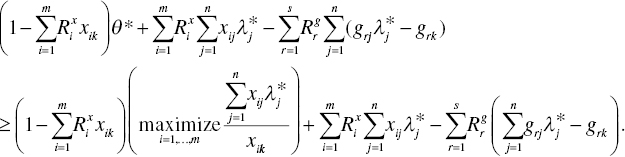
As documented in Table 6.2, the additive model measures the degree of OE by

where λ* is an optimal solution of Model (6.4). The additive model does not use the optimal objective value of Model (6.5) as the degree of OE measure. Hence, let Equation (6.11) be Q(Xk, Gk, X, G, A(X, G), Rh(Xk, Gk)) for the additive model. Then, it is sufficient to show that Equation (6.11) suffers from an occurrence of multiple optimal solutions in Model (6.4).
(a) Source: Sueyoshi and Sekitani (2009).
| DMU | Input | Desirable output |
| {A} | 1 | 2 |
| {B} | 2 | 3 |
| {C} | 2 | 1/10 |
The optimal objective value of the additive model (6.4), applied to DMU {C}, becomes –2.9. The optimal solution needs to satisfy ![]() .
.
Hence, Equation (6.11) becomes

The above inequalities indicate that the additive model applied to DMU {C} suffers from an occurrence of multiple OE measures. The upper and lower bounds are specified by Equation (6.12).
6.6.4 Formal Definitions on Other Desirable Properties
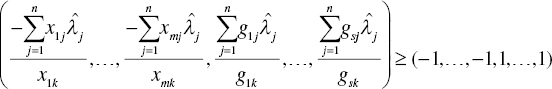
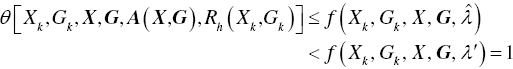
The preceding subsections have discussed which model satisfies the three properties (i.e., aggregation, frontier shift measurability and invariance to alternate optima). To examine the other desirable properties, let θ[Xk, Gk, X, G, A(X, G), Rh(Xk, Gk)] be the OE measure of the k‐th DMU by all DEA models. The OE measure (θ) is equivalent to Q[Xk, Gk, X, G, A(X, G), Rh(Xk, Gk)] in all DEA models except RAM and the additive model. In RAM, for example, the OE measure is ![]() Using this formulation, this chapter defines the remaining desirable properties as follows:
Using this formulation, this chapter defines the remaining desirable properties as follows:
- Homogeneity (input‐oriented): For each DMU k with
 (i.e., inefficient), every optimal solution λ* in Model (6.1) needs to satisfy
 - Strict Monotonicity: For all DMUs k with
 (so, being inefficient), any optimal solution (λ*) in Model (6.1) needs to satisfyHere,
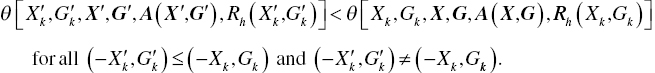
 and
and  .
. - Efficiency Requirement: All DMUs k need to satisfyEven if

 , it may not imply the status of efficiency and the DMU k may not have any feasible solution on λ in Model (6.1) such that
  ,
,  and
and  .
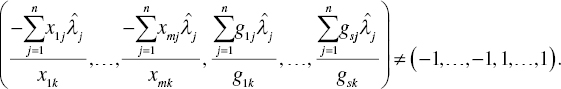
. - Unique Projection for Efficiency Comparison: There exists (X', G') such that
 and
and  for all optimal solutions of λ* in Model (6.1).
 - Unit Invariance: For any positive diagonal matrix Dx whose order is m and any positive diagonal matrix Dg whose order is s, all DMUs{k} need to satisfy

- Translation Invariance: For every pair of the m‐dimensional non‐negative vector (πx) and the s‐dimensional nonnegative vector (πg), the following relation:needs to satisfy for all DMUs{k} where

 and
and  .
.

6.6.5 Efficiency Requirement
Proposition 6.1 indicates that SARM may violate the desirable property on efficiency requirement, and Example 6.4 shows that the additive model violates the property. The property on the other DEA models can be summarized as follows:
It is true that both RM(v) and RM(c) have the property of ![]() . However, even if these OE measures (θ) are unity, we cannot immediately conclude that DMU {k} is fully efficient because we need to confirm whether all slacks are zero or not.
. However, even if these OE measures (θ) are unity, we cannot immediately conclude that DMU {k} is fully efficient because we need to confirm whether all slacks are zero or not.
6.6.6 Homogeneity
The property of homogeneity should be discussed only on an inefficient DMU (so, ![]() ). The status change of an efficient DMU due to μ does not have any theoretical implication because the change reorganizes the structure of an efficiency frontier.
). The status change of an efficient DMU due to μ does not have any theoretical implication because the change reorganizes the structure of an efficiency frontier.
The non‐radial models violate the property of homogeneity. For instance, this chapter can confirm the violation of RAM by Example 6.5.
(a) Source: Sueyoshi and Sekitani (2009).
| DMU | Input | Desirable output |
| {A} | 1 | 2 |
| {B} | μ | 1/2 |
| {C} | 2 | 1/2 |
In Example 6.5, μ is an arbitrary positive number. If ![]() , then DMU {A} is fully efficient. If
, then DMU {A} is fully efficient. If ![]() , then DMU {C} is fully inefficient. If
, then DMU {C} is fully inefficient. If ![]() , then DMU {B} is fully inefficient. The objective of RAM becomes 1–0.5 μ on DMU {B} if 2
, then DMU {B} is fully inefficient. The objective of RAM becomes 1–0.5 μ on DMU {B} if 2![]() 1 and it is 0 if
1 and it is 0 if ![]() 2. When μ = 1,the OE measure of DMU {B} is 0.5. The homogeneity of RAM for
2. When μ = 1,the OE measure of DMU {B} is 0.5. The homogeneity of RAM for ![]() (1.5, 0.5) has the following relationship:
(1.5, 0.5) has the following relationship:

for all μ such that ![]() and
and

for all ![]() . Hence, RAM does not satisfy the property of homogeneity on
. Hence, RAM does not satisfy the property of homogeneity on ![]() (1.5, 0.5).
(1.5, 0.5).
The following example indicates that SBM and Russell measure violate the property of homogeneity:
(a) Source: Sueyoshi and Sekitani (2009).
| DMU | Input 1 | Input 2 | Output |
| {A} | 1 | 2 | 1 |
| {B} | 5/4 | 1 | 1 |
| {C} | μ | 3 μ | 1 |
In Example 6.6, μ is an arbitrary positive number. If μ![]() 1, then DMUs {A, C} are efficient. If
1, then DMUs {A, C} are efficient. If ![]() , then the OE measure of DMU {B} is
, then the OE measure of DMU {B} is ![]() . If μ = 1, then the inputs and output of DMU {C} become
. If μ = 1, then the inputs and output of DMU {C} become ![]() and
and ![]() . In this case, DMU {B} becomes efficient and the OE measure of DMU {C} is 5/6. Hence, a DMU {k} with
. In this case, DMU {B} becomes efficient and the OE measure of DMU {C} is 5/6. Hence, a DMU {k} with ![]() and
and ![]() has the following OE measure under
has the following OE measure under ![]() :
:

Thus, the SBM violates the property of homogeneity.
The Russell measure of DMU {B} is 8/9. Under ![]() , the OE measure of DMU {B} is
, the OE measure of DMU {B} is ![]() . Thus, the DMU with
. Thus, the DMU with ![]() and
and ![]() has the following OE measure under
has the following OE measure under ![]() :
:

Thus, the Russell measure violates the property of homogeneity.
Note that this chapter does not prove that the additive model and SARM violate the property of homogeneity, but the above proof is applicable to the two DEA models in a similar manner.
6.6.7 Strict Monotonicity
This chapter confirms the second assertion on the violation of RM(c), RM(v) and SARM.
(a) Source: Sueyoshi and Sekitani (2009).
| DMU | Input | Desirable output 1 | Desirable output 2 |
| {A} | 1 | 2 | 1 |
| {B} | 2 | μ | 1 |
In Example 6.7, μ is an arbitrary positive number less than 2. Let us consider a case in which input‐oriented RM(c) is applied to DMU {B}. The constraints related to the desirable outputs become ![]() ,
, ![]() ,
, ![]() and
and ![]() . Since μ is an arbitrary number that is less than 2,
. Since μ is an arbitrary number that is less than 2, ![]() becomes redundant. The optimal solution
becomes redundant. The optimal solution ![]() satisfies
satisfies ![]() . Hence, if
. Hence, if ![]() , then the optimal solution of DMU{B} is
, then the optimal solution of DMU{B} is ![]() . The optimal objective value is 0.5. The OE measure of DMU {B} is invariant even if the first output is reduced. Thus, the RM(c) violates the property of strict monotonicity. The violation of other radial models [e.g., RM(v) and SARM] is found in a similar manner.
. The optimal objective value is 0.5. The OE measure of DMU {B} is invariant even if the first output is reduced. Thus, the RM(c) violates the property of strict monotonicity. The violation of other radial models [e.g., RM(v) and SARM] is found in a similar manner.
In addition to the radial models, it is necessary for us to prove that both RAM and the additive model do not satisfy the property of strict monotonicity. Before examining the property, this chapter reviews the statement prepared by Cooper et al. (1999, p. 17) which is written the following: “RAM will also have properties that are referred to as strong monotonicity. We describe this property as follows: Holding all other inputs and outputs constant, an increase in any of its inputs will increase the inefficiency score for an inefficient DMU. The same is true for a decrease in any of its outputs.”
This chapter considers that the comment on RAM’s strict monotonicity is important. However, Example 6.5 shows an example in which the RAM violates the property of strict monotonicity. In Example 6.5, let μ be an arbitrary number which is more than or equal to 1. If ![]() , then DMU {A} is efficient. If
, then DMU {A} is efficient. If ![]() , then DMU {C} is efficient. The efficiency measured by RAM becomes 1–0.5μ if
, then DMU {C} is efficient. The efficiency measured by RAM becomes 1–0.5μ if ![]() and it is 0 if μ
and it is 0 if μ![]() 2. This result indicates that if μ
2. This result indicates that if μ![]() 2, then holding the input and desirable output of the other DMUs, an increase in the input of DMU {B} does not change the efficiency measure (= 0: fully inefficient). Meanwhile, if
2, then holding the input and desirable output of the other DMUs, an increase in the input of DMU {B} does not change the efficiency measure (= 0: fully inefficient). Meanwhile, if ![]() , the efficiency of DMU {B} depends upon an increase of the input. Thus, the RAM does not maintain the property of strict monotonicity. The violation of RAM is because an increase in the i‐th input, while holding the others, simultaneously increases the range adjustment (
, the efficiency of DMU {B} depends upon an increase of the input. Thus, the RAM does not maintain the property of strict monotonicity. The violation of RAM is because an increase in the i‐th input, while holding the others, simultaneously increases the range adjustment (![]() ). Consequently, the level of RAM efficiency is not changed by the input increase. The discussion here is applicable to the desirable output‐based RAM that violates the property of strict monotonicity8. Finally, note that this chapter can prove the violation of strict monotonicity by the additive model in a similar manner.
). Consequently, the level of RAM efficiency is not changed by the input increase. The discussion here is applicable to the desirable output‐based RAM that violates the property of strict monotonicity8. Finally, note that this chapter can prove the violation of strict monotonicity by the additive model in a similar manner.
6.6.8 Unique Projection for Efficiency Comparison
The following examples confirm the violation of unique projection for efficiency comparison:
(a) Source: Sueyoshi and Sekitani (2009).
| DMU | Input 1 | Input 2 | Desirable output |
| {A} | 1 | 2 | 2 |
| {B} | 2 | 1 | 2 |
| {C} | 2 | 2 | 2 |
| {D} | 6 | 6 | 1 |
When RAM, SBM and Russell measure are applied to the data set of Example 6.8, the three models have multiple optimal solutions on DMU {C} such as ![]() . Multiple projections occur on the following line segment:
. Multiple projections occur on the following line segment:

(a) Source: Sueyoshi and Sekitani (2009).
| DMU | Input | Desirable output 1 | Desirable output 2 |
| {A} | 1 | 2 | 1 |
| {B} | 1 | 3 | 1 |
| {C} | 1 | 1 | 1 |
When input‐oriented RM(c) is applied to DMU{C} of Example 6.9, the DMU has unity in the degree of OE. However, the DMU suffers from an occurrence of multiple solutions on the following line segment:

Thus, the RM(c) suffers from an occurrence of multiple projections. The assertion is applicable to input‐oriented RM(v), as well. Therefore, the radial measures violate the property of unique projection.
(a) Source: Sueyoshi and Sekitani (2009).
| DMU | Input | Desirable output 1 | Desirable output 2 |
| {A} | 1 | 1 | 2 |
| {B} | 1 | 2 | 1 |
| {C} | 2 | 1 | 1 |
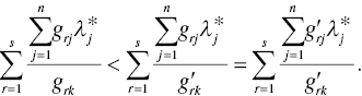
The optimal solution of SARM applied to DMU {C} of Example 6.10 is on ![]() Hence,
Hence, 
![]() becomes a projection point set for DMU {C}. In other words, a projection point(s) of the DMU is not unique and the projection(s) may occur on a line segment:
becomes a projection point set for DMU {C}. In other words, a projection point(s) of the DMU is not unique and the projection(s) may occur on a line segment:  . The discussion on the above three examples can be applied to other DEA models, including the additive model.
6.6.9 Unit Invariance
(a) Source: Sueyoshi and Sekitani (2009).
| DMU | Input | Desirable output |
| {A} | 10 (1/10) | 2 |
| {B} | 20 (2/10) | 3 |
| {C} | 20 (2/10) | 3/2 |
When the additive model is applied to the data set listed in Example 6.11, the optimal solution on DMU {C} becomes ![]() . The optimal objective value is –10.5. Using Model (6.4), this chapter identifies that the OE measure is 3/8. Here, let us consider another data set in which the inputs are divided by 100. The data set is listed within parentheses in Example 6.11. Using the data set, the additive model applied to DMU {C} produces a unique optimal solution:
. The optimal objective value is –10.5. Using Model (6.4), this chapter identifies that the OE measure is 3/8. Here, let us consider another data set in which the inputs are divided by 100. The data set is listed within parentheses in Example 6.11. Using the data set, the additive model applied to DMU {C} produces a unique optimal solution: ![]() . The optimal objective value is –1.5. By transforming the objective value by Model (6.4), the OE measure becomes 0.5. Hence, the additive model violates the property of unit invariance.
. The optimal objective value is –1.5. By transforming the objective value by Model (6.4), the OE measure becomes 0.5. Hence, the additive model violates the property of unit invariance.
6.6.10 Translation Invariance
The following example confirms the assertion. That is, input‐oriented RM(v), RM(c), SARM, SBM and the Russell measure violate the property of translation invariance.
(a) Source: Sueyoshi and Sekitani (2009).
| DMU | Input | Desirable output |
| {A} | 3 (4) | 2 |
| {B} | 4 (5) | 1 |
| {C} | 7/2 (9/2) | 2 |
DMU {C} has the optimal solution ![]() = (1, 0, 0) under RM(c), RM(v), RAM, SARM, SBM and the Russell measure. The OE measure is 3/7 by the two radial models, SARM and SBM. The OE of Russell measure is 0.655. To examine whether these DEA models satisfy the property of translation invariance, this chapter adds one to the three input values, as listed in the second (input) column of Example 6.12. The optimal solution of DMU {C} becomes
= (1, 0, 0) under RM(c), RM(v), RAM, SARM, SBM and the Russell measure. The OE measure is 3/7 by the two radial models, SARM and SBM. The OE of Russell measure is 0.655. To examine whether these DEA models satisfy the property of translation invariance, this chapter adds one to the three input values, as listed in the second (input) column of Example 6.12. The optimal solution of DMU {C} becomes ![]() = (1, 0, 0) under the five DEA models, but the optimal objective value, indicating the degree of OE, becomes 4/9. The OE measure of Russell measure becomes 2/3. Thus, the two radial models, SARM, SBM and the Russell measure do not satisfy the property of translation invariance.
= (1, 0, 0) under the five DEA models, but the optimal objective value, indicating the degree of OE, becomes 4/9. The OE measure of Russell measure becomes 2/3. Thus, the two radial models, SARM, SBM and the Russell measure do not satisfy the property of translation invariance.
The following example confirms the assertion on the additive model:
(a) Source: Sueyoshi and Sekitani (2009).
| DMU | Input | Desirable output |
| {A} | 3 (4) | 1 |
| {B} | 4 (5) | 1 |
The additive model, applied to DMU {B} in Example 6.13, produces ![]() as an optimal solution and –1 as an optimal objective value of Model (6.4). The objective value is changed to 7/8 as the OE measure. If we add one to the two input values, as listed in the second (input) column of Example 6.13, then the additive model applied to DMU {B} produces
as an optimal solution and –1 as an optimal objective value of Model (6.4). The objective value is changed to 7/8 as the OE measure. If we add one to the two input values, as listed in the second (input) column of Example 6.13, then the additive model applied to DMU {B} produces ![]() as the optimal solution and –1 as the optimal objective value of Model (6.4). However, the OE measure becomes 9/10. Hence, the additive model violates the property of translation invariance.
as the optimal solution and –1 as the optimal objective value of Model (6.4). However, the OE measure becomes 9/10. Hence, the additive model violates the property of translation invariance.
6.7 SUMMARY
This chapter reviewed desirable properties for OE in a unified analytical synthesis. Then, we theoretically compared seven radial and non‐radial DEA models based upon the OE criteria. The findings on OE criteria were summarized in Table 6.1. This table provided us with the following guidance in selecting an appropriate DEA model. First, there is no perfect DEA model that can satisfy all desirable OE properties. It is necessary for us to develop the perfect DEA model that can satisfy all the desirable OE properties. That will be important but being a difficult future research task. Second, all DEA models violate both the property of unique projection for efficiency comparison and the property of aggregation. Cooper et al. (2007a) discussed how to deal with the aggregation issue. Third, the additive model violates all desirable OE properties. This chapter recommends the use of RAM as an extended formulation of the additive model because RAM satisfies several desirable OE properties. Fourth, both the Russell measure and SBM (= ERGM) perform as well as RAM as a non‐radial measure. If we are interested in the property of strict monotonicity, the two models (SBM and Russell measure) outperform the other models including RAM. In contrast, if we are interested in the property of translation invariance, RAM outperforms the Russell measure and SBM (= ERGM). In Section II (DEA environmental assessment), the proposed DEA model for non‐radial measurement originates from the RAM because it needs to utilize the property of translation invariance. See Chapter 26 which discusses how to handle an occurrence of many zeros in a data set. Fifth, if we are interested in the property of homogeneity, the two RMs are useful for such a purpose. All the non‐radial models do not satisfy the desirable property9. Sixth, RM(c) is useful in measuring a frontier shift among different periods10. See Chapter 19 which describes how to measure a frontier shift among different periods by using the radial measurement for environmental assessment, under constant RTS. Finally, if a data set contains zero and/or negative values, then we need to depend upon the property of “disaggregation” although this chapter has not discussed it. See Chapter 27 for a detailed description on the property of disaggregation. In the case of non‐radial measurement, RAM becomes an appropriate model for the data set11 that contains zero and/or negative values. Meanwhile, in the case of both radial and non‐radial measurements, the property of disaggregation is useful in handling such zero and/or negative values.
In addition to the above implications for DEA users, Table 6.1 indicates that all DEA models examined in this chapter suffer from an occurrence of multiple projections. As a result of such a difficulty, all the DEA models cannot uniquely determine the OE measure for efficiency comparison. The difficulty is often associated with an occurrence of multiple reference sets and multiple projections. Unfortunately, the research issue has been insufficiently explored in previous DEA studies. To overcome the difficulty, we need to develop a new approach that can identify the existence of unique projection for efficiency comparison. The proposed approach combines a DEA model (primal formulation) with its dual model and then adds SCSCs in a combined model. The incorporation of SCSCs restricts projections of an inefficient DMU in a “minimum face” on an efficiency frontier when it changes its status from inefficiency to efficiency. Consequently, the combined primal/dual model with SCSCs can identify a projection set as the minimum face on an efficiency frontier. See Chapter 7 that discusses how to incorporate the SCSCs into DEA assessment.
At the end of this chapter, it is necessary to describe the following four concerns for research extension from conventional DEA to its environmental assessment. First, chapters in Section II need to incorporate undesirable outputs in their computational frameworks. Unification between desirable and undesirable outputs will be very important in terms of DEA environmental assessment. See Chapters 15, 16 and 17 on output unification. Second, a unified efficiency measure for environmental assessment has the assumption that undesirable outputs are “by‐products” of desirable outputs. As a result of the assumption, a desirable output vector should have an increasing trend, and an undesirable output vector should have an increasing and decreasing trend along with an increase in an input vector. To identify an occurrence of such an increasing and decreasing trend, DEA environmental assessment needs to incorporate the concept of “congestion.” See Chapters 9, 20, 21, 22 and 23. Thus, “strict monotonicity” and “liner homogeneity,” for example, are desirable properties for conventional DEA as discussed in this chapter, but are not necessary for environmental assessment. Third, this chapter did not discuss that dual variables, or multipliers, obtained from a radial or non‐radial model should be positive in their signs. Otherwise, production factors, corresponding to dual variables with zero, will be not utilized in DEA assessment. RAM and SARM can satisfy the property. Therefore, the two models will be utilized for non‐radial and radial models for environmental assessment, respectively. Finally, all models used for environmental assessment should be intuitively and visually discussed. As explored in this chapter, DEA environmental assessment will consider a balance between theory and practicality. These concerns will be explored in chapters in Section II.
APPENDIX
Proof of Proposition 6.1
Any combination between ![]() ,
, ![]() and
and ![]() becomes a feasible solution. The objective function
becomes a feasible solution. The objective function ![]() is bounded, because
is bounded, because ![]() and
and ![]() (j = 1, 2,…, n). If
(j = 1, 2,…, n). If ![]() , then SARM does not have an optimal solution. In contrast, if
, then SARM does not have an optimal solution. In contrast, if ![]() , then the objective function of SARM has a lower bound because
, then the objective function of SARM has a lower bound because

Let (θ*, λ*) be an optimal solution of SARM, then ![]() ,
, ![]() and
and ![]() . It follows from
. It follows from ![]() that
that  ∀ = 1,⋯,m. This indicates that
  is a feasible solution of SARM and
 ![]() . Hence, the following relationship is maintained on optimality:
. Hence, the following relationship is maintained on optimality:
The above relationship implies that  is on the optimality of SARM.
Q.E.D.
Proof of Proposition 6.6
For any ![]() ,
, ![]() is maintained in two RMs (input‐oriented), SBM and the Russell measure. For a feasible solution of λ, RAM has
is maintained in two RMs (input‐oriented), SBM and the Russell measure. For a feasible solution of λ, RAM has ![]() ,
, ![]() (i = 1,…, m) and
(i = 1,…, m) and ![]() (r = 1,…, s). Hence,
(r = 1,…, s). Hence, ![]() The solution of
The solution of ![]() and
and ![]() is feasible in two RMs (input‐oriented), SBM and the Russell measure. For a feasible solution of λ, two RMs (input‐oriented), SBM and the Russell measure have
is feasible in two RMs (input‐oriented), SBM and the Russell measure. For a feasible solution of λ, two RMs (input‐oriented), SBM and the Russell measure have ![]() . Hence, RAM has
. Hence, RAM has ![]() and two RMs, SBM and Russell measure have
and two RMs, SBM and Russell measure have ![]() . In other words, two RMs (input‐oriented), RAM, SBM and Russell measure have
. In other words, two RMs (input‐oriented), RAM, SBM and Russell measure have ![]() .
.
Next, we prove that if ![]() is identified by SARM, RAM, SBM and Russell measure, then DMU {k} is fully efficient by using contradiction. We assume that there exists a feasible solution
is identified by SARM, RAM, SBM and Russell measure, then DMU {k} is fully efficient by using contradiction. We assume that there exists a feasible solution ![]() of Model (6.1)for DMU {k} such that
of Model (6.1)for DMU {k} such that ![]() ,
, ![]() and
and ![]() . Since X > 0 and G > 0, we have
. Since X > 0 and G > 0, we have
and
Let ![]() and
and ![]() for all
for all ![]() , then we have
, then we have
for SBM and Russell measure. This is in contradiction to ![]()
![]() .
.
Similarly, we have

and

Therefore, SARM has

and RAM has

This is in contradiction to ![]() .
.
Q.E.D.
Proof of Proposition 6.7
Both of the two input‐oriented RMs have A(X,G) = A(X′,G′) and Rh(Xk, Gk) = Rh(μXk, Gk). Let λ* be an optimal solution in Model (6.1). Then we have ![]() and
and ![]() . It follows from
. It follows from ![]() and
and ![]() that
that

Since 
![]() is maintained in the above equation, we have
is maintained in the above equation, we have

Q.E.D.
Proof of Proposition 6.8
Let λ* be an optimal solution of Model (6.1) for SBM, then we have ![]() . It follows from the definitions of
. It follows from the definitions of ![]() and
and ![]() ,
, ![]() and
and ![]() that
that ![]() . Therefore, λ* is a feasible solution of
. Therefore, λ* is a feasible solution of

where ![]() is an (i,j) component of X' and g' rj is an (r,j) component of G'. Since
is an (i,j) component of X' and g' rj is an (r,j) component of G'. Since ![]() , we have
, we have

Since ![]() , we have either
, we have either

or
Therefore, it follows that

The satisfaction of the Russell measure can be proved in a similar manner. Q.E.D.
Proof of Proposition 6.10
![]() is equivalent to
is equivalent to ![]() . The objective function of two input‐oriented RMs, SBM and the Russell measure consists of
. The objective function of two input‐oriented RMs, SBM and the Russell measure consists of ![]() (i = 1,…, m) and
(i = 1,…, m) and ![]() (r =1,…, s). Let
(r =1,…, s). Let ![]() be an (i,i) component of Dx and let
be an (i,i) component of Dx and let ![]() an (r,r) component of Dg, then we have
an (r,r) component of Dg, then we have ![]() (i = 1,…, m) and
(i = 1,…, m) and ![]()
![]() (r = 1,…, s). Both
(r = 1,…, s). Both ![]() and
and ![]() are unit invariant. Therefore, two input‐based RMs, SBM and the Russell measure are unit invariant.
are unit invariant. Therefore, two input‐based RMs, SBM and the Russell measure are unit invariant.
The objective function of RAM and SARM consists of ![]() and
and ![]() . Since
. Since ![]() for DxX is
for DxX is ![]() (i =1,…, m) and
(i =1,…, m) and ![]() for DgG is
for DgG is ![]() , we have
, we have ![]() and
and ![]() . Therefore, both RAM and SARM are unit invariant.
. Therefore, both RAM and SARM are unit invariant.
Q.E.D.
Proof of Proposition 6.11
For RAM, ![]() is equivalent to
is equivalent to ![]()
![]() . The objective function of RAM consists of
. The objective function of RAM consists of

Since ![]() , we have
, we have
for i = 1,…, m, where πi is the i‐th component of a m‐dimensional non‐negative vector (π).
In the same manner, we can prove ![]() (grk + ψr) for all r = 1,…, s, where ψr is the r‐th component of an s‐dimensional non‐negative vector ψ. From the definitions, the range of
(grk + ψr) for all r = 1,…, s, where ψr is the r‐th component of an s‐dimensional non‐negative vector ψ. From the definitions, the range of ![]() and the range of
and the range of ![]() are equal to those of
are equal to those of ![]() and
and ![]() , respectively. Therefore, we have
, respectively. Therefore, we have

for every k = 1,…, n.
Q.E.D.