
18
SCALE EFFICIENCY
18.1 INTRODUCTION
This chapter1 describes how to measure the degree of scale efficiency under natural or managerial disposability. Scale efficiency indicates a managerial level regarding how each DMU can control its operational size in such a manner that it can enhance the level of unified efficiency.
To document the practicality of the proposed scale efficiency measurement, this chapter applies it to examine the performance of coal‐fired power plants in the north‐east region of the United States. This chapter is also interested in examining whether there is a significant difference between the two types (BIT: bituminous coal and SUB: subbituminous coal) of coal‐fired power plants in their unified efficiency measures, including their scale efficiency measures, under natural and managerial disposability concepts, respectively. Chapter 17 has discussed the coal‐fired power plants in ISO and RTO. Meanwhile, this chapter is not interested in such regional differences in power plant control, rather being concerned with the type of coal combustion in the power plants. As discussed in Chapter 14, the north‐east region (e.g., West Virginia) is controlled by PJM. The PJM, as the most well‐known Regional Transmission Organization (RTO) in the United States, covers areas near the Appalachian Mountains which produce a large amount of SUB. The operation of PJM mainly uses SUB combustion in its coal‐fired power plants. Consequently, the research concern of this chapter is whether such a fuel structure has a difficulty from the perspective of environmental assessment. This chapter is also interested in measuring the scale efficiency of coal‐fired power plants, along with unified efficiency under natural or managerial disposability.
The remainder of this chapter is organized by the following structure. Section 18.2 discusses how to measure the degree of scale efficiency by non‐radial models under natural disposability. Section 18.3 shifts it to managerial disposability. Section 18.4 discusses how to measure the degree of scale efficiency by radial models under natural disposability. Section 18.5 changes it to managerial disposability. Section 18.6 measures the performance of coal‐fired power plants in the United States. Section 18.7 summarizes this chapter.
18.2 SCALE EFFICIENCY UNDER NATURAL DISPOSABILITY: NON‐RADIAL APPROACH
To examine how each DMU carefully manages the operational size under natural disposability, this chapter measures the degree of scale efficiency by
where SEN is scale efficiency under natural disposability which is measured by a non‐radial model (NR). ![]() is unified efficiency under natural disposability that is measured by Model (16.20).
is unified efficiency under natural disposability that is measured by Model (16.20). ![]() is the unified efficiency under natural disposability that is measured by Model (16.20) without
is the unified efficiency under natural disposability that is measured by Model (16.20) without ![]() . Since
. Since ![]() , SENNR is less than or equals unity in the degree of scale efficiency. The higher score in SEN indicates the better scale management under natural disposability.
, SENNR is less than or equals unity in the degree of scale efficiency. The higher score in SEN indicates the better scale management under natural disposability.
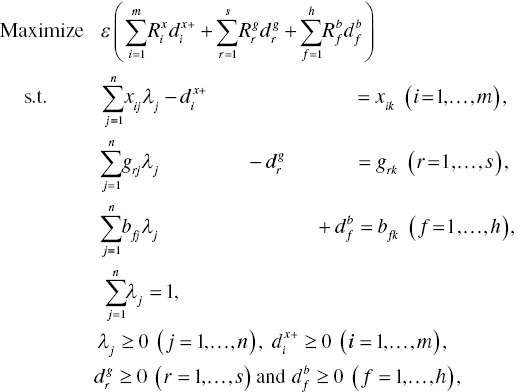
As mentioned above, this chapter uses Model (16.20) for the proposed empirical study that is formulated by the following non‐radial model under natural disposability:


As discussed in Chapter 16, a drawback of the non‐radial approach is that it produces efficient and inefficient DMUs whose unified efficiency measures are very close to unity. To overcome the problem, this chapter adds a small number (ε) to control the magnitude of unified efficiency under natural disposability. The small number is referred to as the “magnitude control factor (MCF)” in Chapter 16.
The unified efficiency (![]() ) of the k‐th DMU under natural disposability and variable RTS is measured by
) of the k‐th DMU under natural disposability and variable RTS is measured by

where all slack variables are determined on the optimality of Model (18.2). The equation within the parenthesis, obtained from the optimality of Model (18.2), indicates the level of unified inefficiency under natural disposability. The unified efficiency is obtained by subtracting the level of inefficiency from unity, as formulated in Equation (18.3).
Meanwhile, the unified efficiency (![]() ) of the k‐th DMU, incorporating constant RTS, is measured by
) of the k‐th DMU, incorporating constant RTS, is measured by

Model (18.4) drops ![]() from Model (18.2), so incorporating constant RTS. See Chapter 20 for a description of RTS. The degree of
from Model (18.2), so incorporating constant RTS. See Chapter 20 for a description of RTS. The degree of ![]() is determined by Equation (18.3). Thus, we can identify the degree of scale efficiency by Equation (18.1), or
is determined by Equation (18.3). Thus, we can identify the degree of scale efficiency by Equation (18.1), or ![]() , by using the proposed two non‐radial models, or Models (18.2) and (18.4).
, by using the proposed two non‐radial models, or Models (18.2) and (18.4).
Figure 18.1 visually describes two efficiency frontiers under variable and constant RTS in the horizontal axis (an input) and the vertical axis (a desirable output). Figure 18.1, corresponding to Stage I (A) of Figure 15.6, assumes that all DMUs use the same amount of an undesirable output, so being not listed in the x–g dimension.

FIGURE 18.1 Two efficiency frontiers under different RTS . (b) See Figure 15.6. This figure corresponds to Stage I (A) of Figure 15.6. (c) This figure is prepared for a desirable output‐oriented case. (d) RTS stands for returns to scale.
(a) Source: Sueyoshi and Goto (2015b). This study updates the original work
In Figure 18.1, the straight line from the origin to a projected production point, or G (passing DMU {B}), is an efficiency frontier under constant RTS, while DMUs {A, B, C, D, E} consist of the frontier under variable RTS. A production possibility set under variable RTS consists of the region Ω1, while that of constant RTS comprises all three regions (![]() ). DMU {F} is inefficient. The DMU needs to shift the performance from {F} to {C} under variable RTS and to G under constant RTS. This chapter measures the degree of
). DMU {F} is inefficient. The DMU needs to shift the performance from {F} to {C} under variable RTS and to G under constant RTS. This chapter measures the degree of ![]() by the distance {F} to H divided by the distance {C} to H. Meanwhile, the degree of
by the distance {F} to H divided by the distance {C} to H. Meanwhile, the degree of ![]() is measured by the distance {F} to H divided by that of G to H. Here, the location of H is for an artificially created production point which uses an amount of input but has no production on the desirable output. Consequently, we have the following visual relationship in Figure 18.1:
is measured by the distance {F} to H divided by that of G to H. Here, the location of H is for an artificially created production point which uses an amount of input but has no production on the desirable output. Consequently, we have the following visual relationship in Figure 18.1:
The degree of SENNR is less than or equals unity. The status of unity in SENNR implies that a DMU operates under constant RTS in terms of desirable outputs.
18.3 SCALE EFFICIENCY UNDER MANAGERIAL DISPOSABILITY: NON‐RADIAL APPROACH
To measure how each DMU carefully manages the operational size under managerial disposability, this chapter measures the degree of scale efficiency by
where SEMNR is scale efficiency under managerial disposability. ![]() is unified efficiency under managerial disposability as measured by Model (16.21).
is unified efficiency under managerial disposability as measured by Model (16.21). ![]() is the unified efficiency under managerial disposability, measured by Model (16.21) without
is the unified efficiency under managerial disposability, measured by Model (16.21) without ![]() , which incorporates constant DTS. See Chapter 20 for a detailed description on DTS. Since
, which incorporates constant DTS. See Chapter 20 for a detailed description on DTS. Since ![]() , SEMNR is less than or equal to unity. The higher score in SEMNR indicates the better scale management under managerial disposability.
, SEMNR is less than or equal to unity. The higher score in SEMNR indicates the better scale management under managerial disposability.
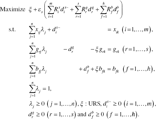
This chapter uses Model (16.21) for the proposed empirical study that is formulated by the following non‐radial model under managerial disposability:
where a prescribed small number (ε) is incorporated into Model (18.6) to control the magnitude of unified efficiency under managerial disposability.
The unified efficiency (![]() ) of the k‐th DMU under managerial disposability and variable DTS is measured by
) of the k‐th DMU under managerial disposability and variable DTS is measured by

where all slack variables are determined on the optimality of Model (18.6). The equation within the parentheses, obtained from the optimality of Model (18.6), indicates the level of unified inefficiency under managerial disposability. The unified efficiency is obtained by subtracting the level of inefficiency from unity, as formulated in Equation (18.7).
Meanwhile, the unified efficiency (![]() ) of the k‐th DMU, incorporating constant DTS, is measured by
) of the k‐th DMU, incorporating constant DTS, is measured by

Model (18.8) drops ![]() from Model (18.6), so incorporating constant DTS. The degree of
from Model (18.6), so incorporating constant DTS. The degree of ![]() is determined by Equation (18.7). Thus, this chapter can identify the degree of scale efficiency by Equation (18.5), or
is determined by Equation (18.7). Thus, this chapter can identify the degree of scale efficiency by Equation (18.5), or ![]() .
.
Figure 18.2, corresponding to Stage I (B) in Figure 15.6, visually describes two efficiency frontiers under constant and variable DTS in the horizontal axis (input : x) and the vertical axis (undesirable output : b). The figure assumes that all DMUs produce the same amount of a desirable output (g), so being not listed in the x–b dimension. The straight line from the origin to a projected point (G, passing on {B}) is an efficiency frontier under constant DTS, while DMUs {A, B, C, D, E} consist of the frontier under variable DTS. A pollution possibility set under variable DTS consists of the region Ω1, while that of constant DTS comprises all three regions (![]() ). DMU {F} is inefficient. The DMU needs to shift the performance from {F} to {C} under variable DTS and to G under constant DTS. This chapter measures the degree of
). DMU {F} is inefficient. The DMU needs to shift the performance from {F} to {C} under variable DTS and to G under constant DTS. This chapter measures the degree of ![]() by the distance {C} to H divided by the distance {F} to H. Meanwhile, the degree of
by the distance {C} to H divided by the distance {F} to H. Meanwhile, the degree of ![]() is measured by the distance G to H divided by that of {F} to H. The H is an artificially created production point which uses an amount of input (x) but it does not produce any pollution. Consequently, this chapter has the following relationship in Figure 18.2:
is measured by the distance G to H divided by that of {F} to H. The H is an artificially created production point which uses an amount of input (x) but it does not produce any pollution. Consequently, this chapter has the following relationship in Figure 18.2: ![]() = (Distance G to H)/(Distance C to H). Here, it is important to note that such a specification on SEMNR in Figure 18.2 is visually opposite to that of SENNR = (Distance C to H)/(Distance G to H) in Figure 18.1.
= (Distance G to H)/(Distance C to H). Here, it is important to note that such a specification on SEMNR in Figure 18.2 is visually opposite to that of SENNR = (Distance C to H)/(Distance G to H) in Figure 18.1.

FIGURE 18.2 Two efficiency frontiers under different DTS (b) See Figure 15.6. This figure corresponds to Stage I (B) of Figure 15.6. (c) This figure is prepared for an undesirable output‐oriented case. (d) DTS stands for damages to scale.
(a) Source: Sueyoshi and Goto (2015b). This study updates the original work.
18.4 SCALE EFFICIENCY UNDER NATURAL DISPOSABILITY: RADIAL APPROACH
The computational procedure of a radial approach is conceptually similar to that of the non‐radial approach in Sections 18.2 and 18.3, but using Model (17.5) in Chapter 17. Returning to the model, this chapter measures the unified efficiency of the k‐th DMU under natural disposability by duplicating the following formulation:
Here, ξ, which is unrestricted in its sign, stands for the level of inefficiency. εs (e.g., 0.00001) is a very small number used in radial measurement such as Model (18.9), so being different from another small number ε (e.g., 0.1) in non‐radial measurement such as Model (18.2) and others. The very small number (εs) is used for both reducing the influence of total slacks and indicating the lower bounds of all multipliers (dual variables). Meanwhile, the small number (ε) is used to adjust the magnitude of total slacks, so controlling the magnitude of unified inefficiency. Thus, both have different usages under radial and non‐radial measurements. See Chapter 1 that provides the three types of small numbers. See also Chapters 16 and 17 for descriptions on non‐radial and radial models, respectively, for DEA environmental assessment.
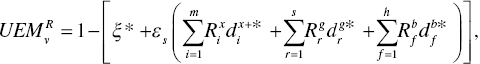
A unified efficiency score (![]() ) of the k‐th DMU under natural disposability is measured by Equation (17.6), or
) of the k‐th DMU under natural disposability is measured by Equation (17.6), or

where the inefficiency score (ξ) and all slack variables are determined on the optimality of Model (18.9). Thus, the equation within the parenthesis is obtained from the optimality of Model (18.9). The unified efficiency under natural disposability is obtained by subtracting the level of inefficiency from unity. The superscript R stands for radial measurement.
Meanwhile, the unified efficiency (![]() ) of the k‐th DMU is measured by
) of the k‐th DMU is measured by

Model (18.11) drops ![]() from Model (18.9), so incorporating constant DTS. The degree of
from Model (18.9), so incorporating constant DTS. The degree of ![]() is determined by
is determined by ![]()
![]() , where the inefficiency score and all the slacks are obtained from the optimality of Model (18.11). Thus, we can identify the degree of scale efficiency by
, where the inefficiency score and all the slacks are obtained from the optimality of Model (18.11). Thus, we can identify the degree of scale efficiency by
where SENR is scale efficiency under natural disposability. ![]() is unified efficiency under natural disposability that is measured by Model (18.9) and
is unified efficiency under natural disposability that is measured by Model (18.9) and ![]() is the unified efficiency under natural disposability that is measured by Model (18.11) with constant RTS.
is the unified efficiency under natural disposability that is measured by Model (18.11) with constant RTS.
18.5 SCALE EFFICIENCY UNDER MANAGERIAL DISPOSABILITY: RADIAL APPROACH
The computational procedure of a radial approach under managerial disposability conceptually follows that of the non‐radial approach, but using Model (17.10) in Chapter 17. Returning to the radial model, this chapter measures the unified efficiency of the k‐th DMU under managerial disposability by duplicating the following formulation:

A unified efficiency score (![]() ) of the k‐th DMU under managerial disposability is measured by Equation (17.11), or
) of the k‐th DMU under managerial disposability is measured by Equation (17.11), or
where the inefficiency score and all slack variables are determined on the optimality of Model (18.13). Thus, the equation within the parenthesis is obtained from the optimality of Model (18.13). The unified efficiency under managerial disposability is obtained by subtracting the level of inefficiency from unity.
Meanwhile, the unified efficiency (![]() ) of the k‐th DMU, incorporating constant DTS, is measured by
) of the k‐th DMU, incorporating constant DTS, is measured by

Model (18.15) drops ![]() from Model (18.13), so incorporating constant DTS in the formulation. The degree of
from Model (18.13), so incorporating constant DTS in the formulation. The degree of ![]() is measured by Equation (18.14), or
is measured by Equation (18.14), or ![]() . Thus, we can identify the degree of scale efficiency by
. Thus, we can identify the degree of scale efficiency by
where SEMR is scale efficiency under managerial disposability. ![]() is unified efficiency under managerial disposability that is measured by Model (18.13) and
is unified efficiency under managerial disposability that is measured by Model (18.13) and ![]() is the unified efficiency under managerial disposability that is measured by Model (18.15) with constant DTS.
is the unified efficiency under managerial disposability that is measured by Model (18.15) with constant DTS.
18.6 UNITED STATES COAL‐FIRED POWER PLANTS
18.6.1 The Clean Air Act
Returning to Table 14.1, Chapter 14 has described the history of the Clean Air Act (CAA) that contains a chronological description on the law. The table summarizes legal actions concerning CAA and their related descriptions from the perspective of energy policy and regulation in the United States. Acknowledging the policy‐making effort of US governments, this chapter needs to mention that it is necessary for us to examine whether the policy implementation of CAA has been effective or not over the pollution control of electric utility firms and their power plant operations. Thus, focusing on the research interest at a plant level, this chapter examines whether CAA implementation really influences the operation of coal‐fired power plants because they are a major group of air polluters in the world.
In addition to air regulation, market liberalization2 is also important for power plant operations. In the United States, the Federal Government (e.g., Federal Energy Regulatory Commission; FERC) has the authority to control both competition at the wholesale level and the promotion of equal access to transmission grids. Meanwhile, Public Utility Commission (PUC) at each state is responsible for restructuring its retail electricity market. In particular, the year (1996) was significantly important in the history of US electric utility regulation because FERC issued Orders 888 and 889 that enabled open access to transmission lines for electricity market participants. Some states (e.g., Rhode Island and California) passed the restructuring legislation on the electric utility industry in 1996. The liberalization policy was due to the economic assertion that competition in the electric power industry would enhance the managerial effort of utility firms to improve their business efficiencies, to reduce consumers’ financial burden and to increase economic prosperity. Thus, electric power firms faced liberalization at federal and state level as well as regulation on their air pollution under the CAA. Figure 18.3 visually summarizes such policy components of the current situation surrounding coal‐fired power plants in the United States.

FIGURE 18.3 Power plant management under different regulation environments. (b) The “liberalization” is a process of market reforms to introduce competition and a less restrictive regulation framework for companies in the electricity industry. (c) The “deregulation” is the modification or repeal of existing regulation or the removal of state control and the introduction of a more formal regulatory framework.
(a) Source: Sueyoshi and Goto (2015b)
Acknowledging the importance of liberalization as a general business trend in the US electric power industry, this chapter needs to mention the existence of an opposite regulatory trend where many states have not yet accepted full retail competition in electricity because of various reasons, such as the California electricity crisis3 and the protection of utility industries and consumers within their states. As mentioned previously, the policy decision regarding electricity restructuring is separated at federal and state levels. Thus, the level of market liberalization depends upon each state in the United States. Consequently, the operation of coal‐fired power plants is classified into either plant operation in liberalized and deregulated states or plant operation in regulated states. Therefore, this chapter focuses upon coal‐fired power plants in PJM (the highly regarded RTO), operating in a liberalized market, which supplies electricity to the north‐east part of the United States. See Chapter 14 which describes the region where PJM provides electricity. Furthermore, an important concern to be examined in this chapter is whether a coal‐fired power plant operates with scale efficiency because the electricity is generated in a large process facility. Thus, proper scale management is important as one of the efficiency enhancement components.
At the end of this subsection, it is important to add that liberalization is a process of market reforms to introduce competition and a less restrictive regulation framework for companies in the electricity industry. In contrast, deregulation is the modification or repeal of existing regulation or the removal of state control and the introduction of a more formal regulatory framework. In the United States, “liberalization” is widely used in descriptions of the electric power industry. Thus, this chapter uses the term hereafter.
18.6.2 Production Factors
In this chapter, the generation of each power plant is characterized by two inputs, a single desirable output and five undesirable outputs. They are considered as production factors. The two inputs are measured by the nameplate capacity (MW: Megawatt) and the amount of annual heat input (mmBtu). The desirable output is measured by the amount of annual net generation (MWh: Megawatt hours). The undesirable outputs are measured by five items: the annual amount of NOx emission (tons), the annual amount of SO2 emission (tons), the annual amount of CO2 emission (tons), the annual amount of CH4 emission (pounds; lbs) and the annual amount of N2O emission (lbs) at each coal‐fired power plant.
Data Accessibility:
The supplementary section of Sueyoshi and Goto (2015) lists the original data set.
The data source is the database4 of EPA’s “eGRID year 2010.” The data set consists of 68 coal‐fired power plants that are operating under the PJM Interconnection. This chapter excludes power plants used for combined heat and power (CHP) and those under mixed combustion with biomass fuel. Descriptive statistics are listed in the research of Sueyoshi and Goto (2015).
In discussing greenhouse gas (GHG) control and performance assessment, this chapter needs to specify the type of GHG emissions, including CO2, methane (CH4), nitrous oxide (N2O), hydrofluorocarbons (HFCs), perfluorocarbons (PFCs) and sulfur hexafluoride (SF6). The SO2 and NOx emissions do not belong to the GHG, but both belong to the acid rain gases that produce major damage on the surface of the earth and in our lives. Thus, it is important for us to pay attention to not only GHG but also acid rain gases whose damage is much more serious than those of the former emissions.
As discussed in Chapter 2, for our computational convenience, each production factor is divided by each factor average for research in this chapter. Such a data treatment is necessary for us in order to avoid the situation where a large production factor dominates the others in the computational process of the proposed DEA environmental assessment. Thus, all production factors are unit‐less in the proposed research. See Chapters 1, 26 and 27 on a description on the data adjustment.
18.6.3 Research Concerns
Table 18.1 summarizes the type of plant primary fuel and the plant capacity factor of 68 power plants. Bituminous coal (BIT)5 is relatively soft coal that contains a tarlike substance, called “bitumen.” Subbituminous coal (SUB) is a type of coal whose properties range from those of lignite to those of bituminous coal. Coal is used primarily as fuel for steam‐electric power generation. The capacity factor of each power plant is the ratio of the actual output over a period to its potential output, if it were possible for it to operate at full nameplate capacity continuously over the same period. The computation of plant capacity factor is defined by [the amount of annual generation (KWh/year)/the number of annual hours (356 days × 24 hours)] × plant capacity (KW).
TABLE 18.1 Plant primary fuel and capacity factor
| No. | Plant name | Plant primary fuel | Plant capacity factor |
| 1 | Shelby Municipal Light Plant | BIT | 0.1928 |
| 2 | Dover | BIT | 0.2003 |
| 3 | Painesville | BIT | 0.1769 |
| 4 | Orrville | BIT | 0.4562 |
| 5 | Whitewater Valley | BIT | 0.2569 |
| 6 | Picway | BIT | 0.0676 |
| 7 | FirstEnergy Rivesville | BIT | 0.0060 |
| 8 | FirstEnergy Willow Island | SUB | 0.0708 |
| 9 | Bremo Bluff | BIT | 0.4421 |
| 10 | FirstEnergy Lake Shore | SUB | 0.3362 |
| 11 | Titus | BIT | 0.3239 |
| 12 | FirstEnergy Albright | BIT | 0.2388 |
| 13 | Niles | BIT | 0.1655 |
| 14 | FirstEnergy Armstrong Power Stat | BIT | 0.5862 |
| 15 | New Castle Plant | BIT | 0.2350 |
| 16 | Joliet 9 | SUB | 0.3997 |
| 17 | Kanawha River | BIT | 0.2964 |
| 18 | FirstEnergy Ashtabula | BIT | 0.2284 |
| 19 | FirstEnergy Mitchell Power Station | BIT | 0.2450 |
| 20 | Sunbury Generation LP | BIT | 0.3976 |
| 21 | FirstEnergy R E Burger | BIT | 0.2236 |
| 22 | Crawford | SUB | 0.4639 |
| 23 | State Line Energy | SUB | 0.6239 |
| 24 | Portland | BIT | 0.3139 |
| 25 | Shawville | BIT | 0.4679 |
| 26 | Cheswick Power Plant | BIT | 0.3193 |
| 27 | Fisk Street | SUB | 0.2669 |
| 28 | East Bend | BIT | 0.7539 |
| 29 | Killen Station | BIT | 0.6713 |
| 30 | Clinch River | BIT | 0.2405 |
| 31 | Kammer | BIT | 0.2401 |
| 32 | Waukegan | SUB | 0.5541 |
| 33 | Avon Lake | BIT | 0.4035 |
| 34 | Indian River Generating Station | BIT | 0.3275 |
| 35 | Clover | BIT | 0.8338 |
| 36 | Big Sandy | BIT | 0.6820 |
| 37 | Tanners Creek | BIT | 0.4050 |
| 38 | Philip Sporn | BIT | 0.2549 |
| 39 | FirstEnergy Fort Martin Power Station | BIT | 0.6278 |
| 40 | Will County | SUB | 0.5206 |
| 41 | FirstEnergy Eastlake | BIT | 0.5698 |
| 42 | Mountaineer | BIT | 0.7090 |
| 43 | Kincaid Generation LLC | SUB | 0.5322 |
| 44 | FirstEnergy Pleasants Power Station | BIT | 0.6916 |
| 45 | Brandon Shores | BIT | 0.5061 |
| 46 | W H Zimmer | BIT | 0.7768 |
| 47 | Walter C Beckjord | BIT | 0.3005 |
| 48 | Miami Fort | BIT | 0.6769 |
| 49 | Muskingum River | BIT | 0.5002 |
| 50 | Morgantown Generating Plant | BIT | 0.5282 |
| 51 | PPL Brunner Island | BIT | 0.7413 |
| 52 | Mitchell | BIT | 0.7161 |
| 53 | PPL Montour | BIT | 0.6675 |
| 54 | Mt Storm | BIT | 0.7015 |
| 55 | Hatfields Ferry Power Station | BIT | 0.5929 |
| 56 | Powerton | SUB | 0.5762 |
| 57 | Cardinal | BIT | 0.6106 |
| 58 | Conemaugh | BIT | 0.7372 |
| 59 | Keystone | BIT | 0.8212 |
| 60 | Conesville | BIT | 0.3900 |
| 61 | Homer City Station | BIT | 0.6245 |
| 62 | FirstEnergy Harrison Power Station | BIT | 0.7001 |
| 63 | J M Stuart | BIT | 0.6268 |
| 64 | FirstEnergy W H Sammis | BIT | 0.5707 |
| 65 | Rockport | SUB | 0.7741 |
| 66 | General James M Gavin | BIT | 0.8292 |
| 67 | FirstEnergy Bruce Mansfield | BIT | 0.7524 |
| 68 | John E Amos | BIT | 0.5988 |
(a) Source: Sueyoshi and Goto (2015b). (b) BIT stands for bituminous coal and SUB stands for subbituminous coal.
The capacity factors of PJM’s 68 coal‐fired power plants, summarized in Table 18.1, indicate two research concerns, summarized by null hypotheses, on the operation of these power plants. One of these research concerns is whether BIT outperforms SUB in terms of coal quality, so producing a lower amount of GHG emission. Therefore, we are interested in examining whether coal‐fired power plants, utilizing BIT, outperform those of SUB in terms of their unified efficiency measures. That is the first hypothesis concerning whether “there is no difference between coal‐fired power plants with BIT and SUB in terms of their unified efficiency measures.”
The other concern is that large coal‐fired power plants may serve as “base‐load,” but small ones cannot be the base‐load power plants in PJM. The base‐load plants provide part of the minimum level of demand on an electrical supply system over 24 hours. Consequently, regulatory agencies (e.g., public utility commission and Environmental Protection Agency; EPA) pay attention to the operation and environmental protection of large power plants, but give limited attention to the small ones. Furthermore, small power plants have more freedom in their bidding strategies than large ones in PJM’s wholesale power market because they are not base‐load power plants. See Chapter 13 which describes a bidding process for wholesale power trading. The concern is summarized by the following second hypothesis on whether there is no difference between coal‐fired power plants with small operation (less than 50% in plant capacity factor) and large operation (more than 50% in plant capacity factor) in their unified efficiency measures. It is generally acceptable to consider that there is a correlation between an operation size and a plant capacity factor, depending upon the type of fuel. The correlation may be found in coal‐fired power generation because they can serve as both base and non‐base load plants.
18.6.4 Unified Efficiency Measures of Power Plants
Table 18.2 summarizes the unified efficiency measures of PJM’s 68 coal fired power plants in 2010. Model (18.2) under natural disposability and Model (18.6) under managerial disposability are used to measure their unified efficiency scores along with scale efficiency measures. The scale efficiency measures are determined by Equation (18.1) under natural disposability and Equation (18.5) under managerial disposability.
TABLE 18.2 Unified efficiencies on power plants: non‐radial approach
(a) Source: Sueyoshi and Goto (2015b). (b) The plant names are listed in Table 18.1. (c) UENv and UENc stand for unified efficiencies, i.e., ![]() and
and ![]() under natural disposability. SEN stands for SENNR under natural disposability. The lowercase v and c stand for variable and constant RTS, respectively. (d) UEMv and UEMc stand for unified efficiencies, i.e.,
under natural disposability. SEN stands for SENNR under natural disposability. The lowercase v and c stand for variable and constant RTS, respectively. (d) UEMv and UEMc stand for unified efficiencies, i.e., ![]() and
and ![]() under managerial disposability. SEM stands for SEMNR under managerial disposability. The lowercase v and c stand for variable and constant DTS, respectively. (e) All unified efficiency scores are measured under non‐radial models with ε = 0.5.
under managerial disposability. SEM stands for SEMNR under managerial disposability. The lowercase v and c stand for variable and constant DTS, respectively. (e) All unified efficiency scores are measured under non‐radial models with ε = 0.5.
| Plant No. | UENv | UENc | SEN | UEMv | UEMc | SEM |
| 1 | 1.000 | 0.996 | 0.996 | 0.998 | 0.996 | 0.998 |
| 2 | 1.000 | 0.996 | 0.996 | 0.997 | 0.992 | 0.995 |
| 3 | 0.999 | 0.996 | 0.997 | 1.000 | 1.000 | 1.000 |
| 4 | 0.987 | 0.983 | 0.997 | 1.000 | 0.971 | 0.971 |
| 5 | 0.997 | 0.994 | 0.997 | 1.000 | 1.000 | 1.000 |
| 6 | 0.999 | 0.996 | 0.997 | 0.999 | 0.997 | 0.998 |
| 7 | 1.000 | 0.997 | 0.997 | 1.000 | 1.000 | 1.000 |
| 8 | 0.996 | 0.993 | 0.997 | 1.000 | 1.000 | 1.000 |
| 9 | 0.989 | 0.987 | 0.998 | 0.990 | 0.977 | 0.987 |
| 10 | 0.995 | 0.992 | 0.997 | 0.997 | 0.989 | 0.992 |
| 11 | 0.990 | 0.988 | 0.997 | 0.993 | 0.980 | 0.987 |
| 12 | 0.989 | 0.986 | 0.997 | 0.994 | 0.974 | 0.979 |
| 13 | 0.985 | 0.982 | 0.997 | 1.000 | 0.981 | 0.981 |
| 14 | 0.979 | 0.976 | 0.997 | 0.981 | 0.971 | 0.990 |
| 15 | 0.986 | 0.984 | 0.997 | 0.995 | 0.976 | 0.981 |
| 16 | 0.987 | 0.985 | 0.998 | 0.992 | 0.965 | 0.972 |
| 17 | 1.000 | 1.000 | 1.000 | 1.000 | 1.000 | 1.000 |
| 18 | 0.986 | 0.984 | 0.997 | 0.997 | 0.970 | 0.973 |
| 19 | 0.990 | 0.987 | 0.998 | 1.000 | 1.000 | 1.000 |
| 20 | 0.964 | 0.961 | 0.998 | 0.975 | 0.899 | 0.922 |
| 21 | 0.980 | 0.977 | 0.998 | 0.994 | 0.962 | 0.967 |
| 22 | 0.986 | 0.984 | 0.998 | 0.995 | 0.965 | 0.970 |
| 23 | 0.971 | 0.970 | 0.998 | 0.973 | 0.946 | 0.971 |
| 24 | 0.976 | 0.973 | 0.998 | 1.000 | 0.986 | 0.986 |
| 25 | 0.959 | 0.957 | 0.998 | 0.967 | 0.937 | 0.968 |
| 26 | 0.979 | 0.977 | 0.998 | 1.000 | 1.000 | 1.000 |
| 27 | 0.986 | 0.983 | 0.998 | 1.000 | 0.981 | 0.981 |
| 28 | 1.000 | 1.000 | 1.000 | 1.000 | 1.000 | 1.000 |
| 29 | 0.982 | 0.981 | 0.998 | 0.987 | 0.954 | 0.966 |
| 30 | 0.981 | 0.979 | 0.998 | 1.000 | 0.976 | 0.976 |
| 31 | 0.978 | 0.975 | 0.997 | 1.000 | 0.989 | 0.989 |
| 32 | 0.979 | 0.978 | 0.999 | 0.988 | 0.934 | 0.946 |
| 33 | 0.971 | 0.967 | 0.996 | 1.000 | 1.000 | 1.000 |
| 34 | 0.976 | 0.974 | 0.998 | 1.000 | 0.971 | 0.971 |
| 35 | 1.000 | 1.000 | 1.000 | 0.970 | 0.967 | 0.997 |
| 36 | 0.968 | 0.968 | 0.999 | 0.970 | 0.953 | 0.983 |
| 37 | 0.965 | 0.964 | 0.999 | 0.986 | 0.950 | 0.963 |
| 38 | 0.968 | 0.966 | 0.998 | 1.000 | 0.976 | 0.976 |
| 39 | 0.960 | 0.959 | 0.999 | 0.970 | 0.958 | 0.988 |
| 40 | 0.961 | 0.960 | 0.999 | 0.981 | 0.877 | 0.893 |
| 41 | 0.950 | 0.949 | 0.999 | 0.961 | 0.925 | 0.962 |
| 42 | 1.000 | 1.000 | 1.000 | 1.000 | 1.000 | 1.000 |
| 43 | 0.932 | 0.932 | 0.999 | 0.954 | 0.835 | 0.875 |
| 44 | 0.980 | 0.980 | 1.000 | 0.993 | 0.980 | 0.987 |
| 45 | 1.000 | 1.000 | 1.000 | 1.000 | 1.000 | 1.000 |
| 46 | 1.000 | 1.000 | 1.000 | 0.991 | 0.988 | 0.997 |
| 47 | 0.917 | 0.916 | 0.998 | 1.000 | 0.861 | 0.861 |
| 48 | 0.971 | 0.971 | 1.000 | 0.984 | 0.956 | 0.971 |
| 49 | 0.917 | 0.917 | 0.999 | 1.000 | 0.909 | 0.909 |
| 50 | 0.975 | 0.975 | 1.000 | 1.000 | 1.000 | 1.000 |
| 51 | 0.952 | 0.952 | 1.000 | 0.964 | 0.924 | 0.958 |
| 52 | 1.000 | 1.000 | 1.000 | 1.000 | 1.000 | 1.000 |
| 53 | 1.000 | 1.000 | 1.000 | 1.000 | 1.000 | 1.000 |
| 54 | 1.000 | 0.988 | 0.988 | 1.000 | 1.000 | 1.000 |
| 55 | 1.000 | 1.000 | 1.000 | 1.000 | 1.000 | 1.000 |
| 56 | 0.930 | 0.930 | 1.000 | 0.958 | 0.784 | 0.819 |
| 57 | 1.000 | 1.000 | 1.000 | 1.000 | 1.000 | 1.000 |
| 58 | 1.000 | 1.000 | 1.000 | 1.000 | 1.000 | 1.000 |
| 59 | 0.982 | 0.981 | 0.999 | 1.000 | 1.000 | 1.000 |
| 60 | 0.947 | 0.947 | 0.999 | 1.000 | 0.901 | 0.901 |
| 61 | 0.912 | 0.911 | 0.999 | 1.000 | 0.897 | 0.897 |
| 62 | 1.000 | 1.000 | 1.000 | 1.000 | 1.000 | 1.000 |
| 63 | 1.000 | 0.959 | 0.959 | 1.000 | 0.952 | 0.952 |
| 64 | 0.950 | 0.949 | 0.999 | 1.000 | 0.856 | 0.856 |
| 65 | 0.925 | 0.923 | 0.998 | 0.940 | 0.767 | 0.815 |
| 66 | 1.000 | 1.000 | 1.000 | 1.000 | 0.973 | 0.973 |
| 67 | 1.000 | 0.972 | 0.972 | 1.000 | 1.000 | 1.000 |
| 68 | 1.000 | 0.971 | 0.971 | 1.000 | 1.000 | 1.000 |
| Total Mean | 0.979 | 0.976 | 0.997 | 0.992 | 0.962 | 0.970 |
| Total S.D. | 0.023 | 0.023 | 0.007 | 0.014 | 0.051 | 0.044 |
| Total Max. | 1.000 | 1.000 | 1.000 | 1.000 | 1.000 | 1.000 |
| Total Min. | 0.912 | 0.911 | 0.959 | 0.940 | 0.767 | 0.815 |
A computational result is summarized in Table 18.2 where S.D. stands for standard deviation. Max. and Min. indicate maximum and minimum unified efficiencies, respectively. In Table 18.2, the coal‐fired power plants under natural and managerial disposability exhibit unity or close to unity (at the level of more than 90%) in their unified efficiency scores. One rationale is that the desirable output (i.e., annual net generation) of power plants is controlled by PJM and undesirable outputs (i.e., five GHGs) are regulated by governmental agencies (e.g., EPA), so that they do not have any major difference in their unified (operational and environmental) performance measures. For example, their unified efficiency measures under natural disposability are 0.979 and 0.976 on average, respectively. These average scores slightly change to 0.992 and 0.962, respectively, when they are measured under managerial disposability. See the bottom of Table 18.2. These unified efficiency measures determine the degree of scale efficiencies as 0.997 and 0.970, on average, under natural and managerial disposability.
18.6.5 Mean Tests
Table 18.3 summarizes the mean tests on unified efficiency measures. The table contains two statistical findings. One of the two findings is that this chapter cannot find any statistical difference between small and large operations in unified efficiencies under natural and managerial disposability concepts. An exception can be found in the unified efficiency under managerial disposability with variable DTS. This is because their plant operations are frequently monitored by US regulatory agencies regardless of their capacity factors or sizes. Thus, this chapter cannot statistically reject the second hypothesis.
TABLE 18.3 Mean tests on unified efficiencies: non‐radial approach
(a) Source: Sueyoshi and Goto (2015b). (b) See the notes in the header of Table 18.2. (c) All unified efficiency scores are measured under non‐radial models with ε = 0.5. (d) An asterisk indicates the significance at the 10% level.
| UENv | UENc | SEN | UEMv | UEMc | SEM | |||||||
| Statistics | Small | Large | Small | Large | Small | Large | Small | Large | Small | Large | Small | Large |
| Avg. | 0.982 | 0.976 | 0.980 | 0.973 | 0.998 | 0.996 | 0.996 | 0.988 | 0.973 | 0.952 | 0.977 | 0.963 |
| St.Dev. | 0.017 | 0.028 | 0.017 | 0.027 | 0.001 | 0.009 | 0.007 | 0.017 | 0.032 | 0.063 | 0.030 | 0.054 |
| t‐score | 1.018 | 1.262 | 0.708 | 2.702* | 1.820 | 1.351 | ||||||
| p‐value | 0.313 | 0.212 | 0.484 | 0.010 | 0.074 | 0.182 | ||||||
| Statistics | BIT | SUB | BIT | SUB | BIT | SUB | BIT | SUB | BIT | SUB | BIT | SUB |
| Avg. | 0.981 | 0.968 | 0.978 | 0.966 | 0.997 | 0.998 | 0.994 | 0.980 | 0.972 | 0.913 | 0.977 | 0.931 |
| St.Dev. | 0.022 | 0.027 | 0.022 | 0.026 | 0.007 | 0.001 | 0.011 | 0.021 | 0.036 | 0.084 | 0.034 | 0.068 |
| t‐score | 1.544 | 1.385 | –1.634 | 2.209* | 2.280* | 2.226* | ||||||
| p‐value | 0.147 | 0.189 | 0.107 | 0.049 | 0.044 | 0.048 | ||||||
The other finding is that Table 18.3 statistically confirms that coal‐fired power plants using BIT outperformed the other plants using SUB in the three unified efficiency measures under managerial disposability. This is because the disposability concept has the first priority to environmental performance, so that UEM and SEM exhibit differences depending on the type of the coal combustion. The result also confirms that the quality difference of coal influences the environmental performance of these power plants in PJM. Thus, this chapter can statistically reject the first hypothesis under managerial disposability.
18.7 SUMMARY
This chapter described how to measure the degree of scale efficiency under natural and managerial disposability concepts by using both non‐radial and radial measurements. To document the practicality of scale efficiency, this chapter applied the proposed approach to examine the performance of coal‐fired power plants in the north‐east region of the United States. This chapter confirmed that there was a significant difference between the two types (BIT and SUB) of coal‐fired power plants in their unified efficiency measures, including their scale efficiencies, under the concept of managerial disposability. In contrast, under natural disposability, this chapter could not find such a difference between them. The fact, which BIT outperformed SUB in terms of their unified and scale efficiencies, provides the policy implication that these power plants face a managerial challenge to shift their coal combustions from SUB to BIT in the United States.
Besides the empirical finding, this chapter could not confirm the other hypothesis on whether coal‐fired power plants with small operation (less than 50% of plant capacity) outperformed ones with large operation (more than 50% of plant capacity), and vice versa, in terms of their unified and scale efficiency measures under natural and managerial disposability, with the exception of UEM(v). The rationale was because their plant operations were frequently monitored by US regulatory agencies regardless of their capacity factor or size.
This chapter discussed a methodological issue on DEA applied to energy and environmental assessment. This chapter used ![]() for the proposed non‐radial approach. The use of ε is very important in DEA because it guarantees that all multipliers (dual variables) are positive, along with data ranges, so that information on production factors is fully utilized in the proposed radial and non‐radial approaches6.
for the proposed non‐radial approach. The use of ε is very important in DEA because it guarantees that all multipliers (dual variables) are positive, along with data ranges, so that information on production factors is fully utilized in the proposed radial and non‐radial approaches6.
This chapter used the classification of coal‐fired power plants based upon their plant capacity factors. In the near future, it will be necessary for us to examine other classification methods on the performance of coal‐fired power plants. Such extended investigations are useful in not only the United States but also other industrial nations. In summary, we look forward to seeing a progress in technology innovation, such as clean coal technology7.