7.1 INTRODUCTION

This chapter¹ discusses the importance of strong complementary slackness conditions (SCSCs) in DEA. The use of SCSCs will be extended in Chapter 25 for an assessment on energy utility firms. The methodological concern of Chapter 25 is how to reduce the number of efficient organizations by applying both SCSCs and DEA‐DA (discriminant analysis). See Chapter 11 on DEA‐DA. Thus, this chapter provides a mathematical basis for Chapter 25 (ranking analysis).

To initiate this chapter, we return to Table 6.1 in which at least one DEA model(s) satisfies desirable properties related to OE, except unique projection for efficiency comparison and property of aggregation. The aggregation property, which not all models satisfy, may not be a serious problem in a practical perspective of DEA. An exception may be found in restructuring of industrial organizations, including merger and acquisition (M & A), where the sum of production factors needs to be examined by comparing it with their original achievements by separated firms. This type of managerial issue is very important from a business perspective, but difficult for us to discuss the issue by DEA because it needs to examine the corporate governance of an aggregated organization in a time horizon. A practical approach for discussing the industrial organization issue can be found in Charnes et al. (1988) and Sueyoshi (1991) that discussed how to examine a large‐scale industrial organization issue (e.g., the restructuring policy of telecommunication industry in the United States during the 1980s). See also Sueyoshi et al. (2010). Furthermore, since there are previous research efforts (e.g., Cooper et al., 2007a) on the property of aggregation, this chapter does not discuss the property of aggregation, rather it is directed toward a description on how to handle the occurrence of multiple projections and multiple reference sets as well as the implications of the non‐Archimedean small number (ε_n) from SCSCs that has been not sufficiently examined in previous DEA studies.

Before discussing the implication of SCSCs in DEA, this chapter acknowledges that researchers, including Olesen and Petersen (1996, 2003) and Cooper et al. (2007b), clearly understand the existence of such a problem of multiple projections and reference sets in the OE measurement. However, no previous DEA research has formally explored how to deal with the occurrence of multiple projections, in particular when we cannot access any prior information to restrict the range of dual variables. In this case, we are unable to use multiplier restriction methods such as the AR and CR methods discussed in Chapter 4. As a theoretical extension of Table 6.1, this chapter examines the importance of SCSCs in handling the occurrence of multiple projections and reference sets in this chapter.

This chapter is organized as follows: Section 7.2 describes the combination of primal and dual models for the development of SCSCs. Section 7.3 summarizes illustrative examples on the use of SCSCs. Section 7.4 discusses theoretical implications on SCSCs. Section 7.5 discusses a guideline on how to extend the use of SCSCs from radial to non‐radial measurement. Section 7.6 summarizes this chapter.

7.2 COMBINATION BETWEEN PRIMAL AND DUAL MODELS FOR SCSCs

Using input‐oriented RM(v), or Model (4.4), this chapter can slightly modify it by a vector expression for our descriptive convenience. The modified version can be expressed by the following formulation:

(7.1)

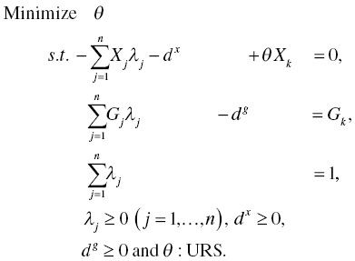
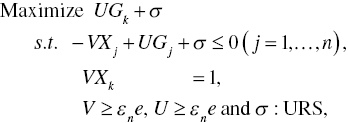
The dual formulation of Model (7.1) is formulated as the following vector expression:

(7.2)

where and are two row vectors of dual variables related to the first and second sets of constraints in Model (7.1). A dual variable (σ), which is unrestricted in the sign, is due to the third constraint of Model (7.1).

Complementary slackness conditions (CSCs) always exist between every optimal solution (θ*, λ*, d^x *, d^g *) of Model (7.1) and every optimal solution (V*, U*, σ*) of Model (7.2). They are specified as follows:

(7.3)

(7.4)

(7.5)

Equation (7.3) multiples –1 on both sides of the first equations of Model (7.2) to maintain (j = 1,…, n). This is for our descriptive convenience.

Pairing the optimal solution (θ*, λ*, d^x *, d^g *) of Model (7.1) with the optimal solution (V*, U*, σ*) of Model (7.2) may satisfy the following additional conditions between them:

(7.6)

(7.7)

(7.8)

In addition to Equations (7.3) to (7.5), satisfaction of the additional conditions in Equations (7.6) to (7.8) implies SCSCs². Thus, the SCSCs consist of Equations (7.3) to (7.8) in the input‐oriented RM(v).

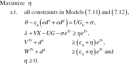
To deal with an occurrence of multiple projections and reference sets, this chapter combines Model (7.1) with Model (7.2) and then adds Equations (7.6) to (7.8). The final model, combining all formulations for SCSCs, becomes as follows:

(7.9)

Here, the superscript Tr indicates a vector transpose. The second equation of Model (7.9) indicates that, for optimality, the objective of Model (7.1) should be equivalent to that of Model (7.2). The last three groups of constraints indicate that an optimal solution obtained from Model (7.9) needs to satisfy the additional conditions required to satisfy SCSCs. A new decision variable (η) is unknown and it is incorporated into Model (7.9) in order to maintain the SCSCs on optimality. See Sueyoshi and Sekitani (2007a, c).

Motivation for Model (7.9):

An underlying rationale regarding why the development of Model (7.9) is necessary for DEA is because of the following rationale. That is, if we face an occurrence of multiple solutions (e.g., multiple projections and multiple reference sets), it is necessary for us to restrict dual variables (multipliers) by a unique projection from inefficiency to efficiency. However, the multiplier restriction methods (i.e., AR and CR), as discussed in Chapter 4, depend upon the availability of prior information (e.g., previous experience). Furthermore, such multiplier restriction methods do not always guarantee a unique projection and a unique reference set. Therefore, it is necessary for us to consider the multiplier restriction without any prior information, consequently dealing with an occurrence of multiple projections and multiple reference sets. That is the rationale concerning why we need SCSCs for conventional DEA.

Here, it is important to note that the incorporation of SCSCs into Model (7.9) does not immediately imply that the optimal solution of Model (7.9) always satisfies the conditions for SCSCs. To satisfy the SCSCs by Model (7.9), the proposed combined model needs to incorporate a new variable (η) that is maximized in Model (7.9). The maximization is necessary because we look for a positive value. Consequently, the optimal solution of Model (7.9) satisfies the SCSCs. It is also true that there is a possibility in which η becomes zero on optimality. In this case, Model (7.9) does not work as we expect. An easy approach to handle the problem can be found in Chapters 16 and 17 that discuss how to avoid the use of SCSCs for DEA environmental assessment by a data range adjustment. See Chapter 26, as well, which discusses a methodological problem of SCSCs from ranking analysis on all DMUs.

A unique reference set covering all possible reference sets:

A benefit of solving Model (7.9), equipped with SCSCs, is that a reference set measured by the model may be considered to be unique because it contains all possible reference sets generated by Model (7.1). It is true that a single reference set does not solve the occurrence of multiple projections. However, the single reference set measured by Model (7.9) can specify the range of multiple projection sets (due to multiple projections) on an efficiency frontier, because Model (7.9) can identify the interior of the convex hull of efficient DMUs within the reference set that covers all possible projection sets. Thus, it is possible for us to identify an occurrence of all possible multiple projections by examining the dimension of such a projection set determined by SCSCs. Further, by examining the reference set of Model (7.9), we can specify which surface on a production possibility set contains all possible projection sets in the interior region even if multiple projections occur.

Positive dual variable on efficient DMUs:

The incorporation of SCSCs into DEA, as formulated by Model (7.9), has two analytical features to be discussed, here. One of the two features is that, if the k‐th DMU is efficient, then (), where RS_k stands for a reference set of the k‐th DMU, is identified for the optimality of Model (7.1). Furthermore, the efficient DMU has (i = 1,…, m) and (r = 1,…, s) for the optimality of Model (7.2). As a result, the efficient DMU has (), (i = 1,..., m) and (r = 1,…, s) for optimality. Thus, the positivity on dual variables is identified without any multiplier restriction methods. That is an important feature of SCSCs incorporated into Model (7.9) that is a combined formulation between Models (7.1) and (7.2). Of course, the positivity on dual variables does not guarantee that Model (7.9) always produces a perfectly acceptable solution. Rather, the model is the first step for avoiding an occurrence of zero on dual variables (multipliers) of efficient DMUs. Such an occurrence is clearly inappropriate and unacceptable in many cases. Thus, DEA equipped with SCSCs can provide us with an opportunity to examine if information on all production factors is fully utilized in the computation process of DEA.

The second feature is that the property for positive dual variables is useful on only an efficient DMU. The property of SCSCs does not function on inefficient DMUs, because an inefficient DMU has usually at least one positive slack (i.e., for some i and for some r)³. Consequently, the proposed SCSCs are not useful on an inefficient DMU. However, the inefficient DMU is not important in terms of making an efficiency frontier, so not determining the degree of OE on the other DMUs. The elimination of the inefficient DMU does not influence the computational process of other DMU’s OE measures. Furthermore, the incorporation of SCSCs may reduce the magnitude of OE on inefficient DMUs because of the restriction on dual variables (multipliers). See Chapter 10 on the computational concern on an inefficient DMU in DEA.

Weakness:

A drawback of Model (7.9) is that it increases the computational burden, compared with Models (7.1) and (7.2), because the former model has more side constraints than the latter ones. The computational issue depends upon a programming capability of a DEA user. Considering the capability of a modern personal computer, such a computational drawback is very minor because Model (7.9) is formulated by linear programming. As long as DEA models are formulated by linear programming, we can easily solve Model (7.9) without any computational difficulty. Such a computational concern belongs to “common sense” for optimization.

Strength:

Model (7.9) has a methodological benefit. As mentioned previously, multipliers (V, W and σ) become positive without depending upon multiplier restriction methods (e.g., the AR and CR approach in Chapter 4) which incorporate prior information into DEA computational process. In other words, Model (7.9) can restrict multipliers (i.e., dual variables) to be positive by the incorporation of SCSCs. This chapter does not discuss such a methodological benefit, rather directing toward how to handle an occurrence of multiple projections and multiple reference sets, hereafter.

7.3 THREE ILLUSTRATIVE EXAMPLES

This chapter uses three illustrative examples to discuss the importance of SCSCs in DEA from different computation concerns.

7.3.1 First Example

The first data set contains six DMUs whose production processes use two inputs to yield a single desirable output. The six DMUs are {A, B, C, D, E, F}, whose two inputs (x₁ and x₂) and one desirable output (g) are

• {A} = (10, 10, 10), {B} = (10, 10, 15), {C} = (8, 10, 14), {D} = (7, 10, 13), {E} = (6, 10, 12), and {F} = (5, 10, 10).

Figure 7.1 depicts the data set in three‐dimensional space.

As depicted in Figure 7.1, the piece‐wise linear concur segments ({B}‐{C}‐{E}‐{F}) consist of an efficiency frontier. The five DMUs, except {A}, are all on the efficiency frontier, so being efficient in terms of the OE measurement. The remaining DMU {A} is inefficient. When we solve DMU {A} by Model (7.1), the following two optimal solutions become feasible in Model (7.1):

and

The first optimal solution indicates a projection from {A} to {E}, while the second one indicates the projection from {A} to {C}. Both indicate that DMU {A} is inefficient because of positive slacks although the efficiency score is unity. The unity in efficiency is due to the fact that Model (7.1) is an input‐oriented model and the second input is 10 for all DMUs. The two results indicate that Model (7.1) produces two different optimal solutions (so, two projections) for DMU {A}. Furthermore, all the points on the line segment between {C} and {E} can become optimal solutions (so, multiple projections) for DMU {A}. Thus, an infinite number of optimal solutions occur on DMU {A} by Model (7.1). This example of Figure 7.1 visually describes such an occurrence of multiple projections in DEA, or Model (7.1).

What is the difficulty in OE measurement?:

An occurrence of multiple projections implies that we must deal with multiple solutions (e.g., multiple comparisons for OE) in Model (7.1). When this type of problem occurs in OE measurement, we cannot uniquely compare the input vector of a DMU with an efficient one because multiple projections produce multiple efficient input vectors. A difficulty in input vector comparison can be easily applied to the occurrence of multiple projections (so, multiple comparisons) on desirable outputs, as well. Consequently, the OE measure of a DMU needs to be determined on an efficiency frontier that contains all possible multiple projections. Furthermore, the occurrence of multiple projections is usually associated with a possible occurrence of multiple reference sets. Such a combined occurrence makes the problem of multiple projections more difficult in DEA performance assessment. It is indeed true that if we pay attention to the level of OE, then an occurrence of multiple projections and reference sets does not produce any major difficulty to us. In contrast, if we are interested in determining the type of returns to scale (RTS) as discussed in Chapter 8 and/or the occurrence of congestion as discussed in Chapter 9, then multiple projections and multiple reference sets become serious problems in not only conventional DEA but also its environmental assessment.

To explain the difficulty due to a simultaneous occurrence of multiple projections and multiple reference sets more clearly in the framework of DEA, this chapter returns to the example of Figure 7.1 in which we identify an occurrence of multiple reference sets for an inefficient DMU {A}. The occurrence depends upon which part of an efficiency frontier the inefficient DMU is projected onto. In Figure 7.1, the line segment between {C} and {E} is part of the efficiency frontier ({B}‐{C}‐{E}‐{F}) onto which DMU {A} may be projected. The set is referred to as a “projection set (Ω),” hereafter. On the line segment (i.e., as a projection set), this chapter can identify that seven possible combinations: {C}, {D}, {E}, {C, D}, {C, E}, {D, E} and {C, D, E} may become possible candidates for a reference set for DMU {A}. This chapter considers DMUs {C, D, E} as a reference set for DMU {A} because it covers all combinations of possible reference sets. Furthermore, the reference set covers all projection sets even if multiple projections occur on DMU {A}.

Practicality of a unique reference set:

Cooper et al. (2006, p. 47) have discussed the importance of examining a reference set because each DMU is relatively evaluated by other DMUs in the reference set. Therefore, the reference set measured by Model (7.1) needs to assume its uniqueness. In contrast, the proposed approach by Model (7.9) does not need such an assumption. For example, returning to Figure 7.1, DMUs {C, D, E} determine the efficiency score of DMU {A} as a reference set. Thus, the proposed approach, equipped with SCSCs, can identify all efficient DMUs that need to be included in the reference set. Such an analytical capability of Model (7.9) can enhance the practicality of DEA in identifying a reference set.

Mathematical expression on a projection set:

To discuss more formally a reference set under an occurrence of multiple projections, this chapter proposes the following two conditions:

1. Condition 1: A reference set should cover all possible reference sets on a projection set (Ω).
2. Condition 2: The convex hull of the reference set should contain Ω.

These two conditions guarantee that we can determine an OE measure based upon a single reference set even if multiple projections occur on a DMU.

Returning to the example of Figure 7.1, it is necessary for us to describe that the problem, due to multiple projections and multiple reference sets, occurs not only on an inefficient DMU such as {A} but also on another efficient DMU {D}. The efficient DMU has multiple reference sets on the line segment on {C}, {D}, and {E}, so having seven possible reference combinations: {C}, {D}, {E}, {C, D}, {C, E}, {D, E} and {C, D, E}. The proposed model (7.9) applied to {A} and {D} produces the results summarized in Table 7.1. Model (7.9) identifies DMUs {C, D, E} as a reference set for inefficient DMU {A} and efficient DMU {D}, but with different weights on intensity variables (). Thus, it is possible for us to specify a single projection on a single reference set. The OE measure of each DMU is determined by comparing its performance with those of efficient DMUs that are identified on a single reference set. As discussed here, Model (7.9) equipped with SCSCs can identify an occurrence of multiple projections by finding a single reference set.

DMU	θ*	λ*	dx *	dg *	Reference Set
{A}	1				{C, D, E}
{D}	1				{C, D, E}

7.3.2 Second Example

Returning to Table 2.4 in Chapter 2, this chapter applies four radial measurements: two models: RM(c) and RM(v) × two cases: with and without SCSCs to the data set for our methodological comparison. First, Table 7.2 duplicates the computational results of Table 2.5 that are solved by input‐oriented RM(c), or Model (2.5). In other words, it corresponds to Model (7.1) without and SCSCs. Second, Table 7.3 summarizes computational results that are solved by input‐oriented RM(v), or Model (7.1). Third, Table 7.4 corresponds to the result of RM(c) with SCSCs. Finally, Table 7.5 corresponds to the result of RM(v) with SCSCs. Although the analytical capability of RM(c) with SCSCs is not discussed in the first illustrative example, this second example describes such an important feature of SCSCs on both RM(v) and RM(c) in our comparative analysis.

Company	DEA Efficiency	Reference Set			u*
{A}	0.833		0.167	0.167	0.833	0.000	0.000	0.000
{B}	0.727		0.182	0.091	0.727	0.000	0.000	0.000
{C}	1		0.000	1	1	0.000	0.000	0.000
{D}	1		0.250	0.125	1	0.000	0.000	0.000
{E}	1		0.500	0.000	1	0.000	0.000	0.000
{F}	1		0.000	1	1	2.000	0.000	0.000

Company	DEA Efficiency	Reference Set			u*
{A}	0.833		0.167	0.167	0.000	0.000	0.000	0.000
{B}	0.727		0.182	0.091	0.000	0.000	0.000	0.000
{C}	1		0.000	1	0.000	0.000	0.000	0.000
{D}	1		0.250	0.125	0.000	0.000	0.000	0.000
{E}	1		0.500	0.000	0.000	0.000	0.000	0.000
{F}	1		0.000	1	0.000	2.000	0.000	0.000

Company	DEA Efficiency	Reference Set			u*
{A}	0.833		0.167	0.167	0.833	0.000	0.000	0.000
{B}	0.727		0.182	0.091	0.727	0.000	0.000	0.000
{C}	1		0.167	0.333	1	0.000	0.000	0.000
{D}	1		0.231	0.154	1	0.000	0.000	0.000
{E}	1		0.300	0.100	1	0.000	0.000	0.000
{F}	1		0.000	1	1	1.000	0.000	0.000

Company	DEA Efficiency	Reference Set			u*
{A}	0.833		0.167	0.167	0.167	0.000	0.000	0.000
{B}	0.727		0.182	0.091	0.091	0.000	0.000	0.000
{C}	1		0.167	0.333	0.167	0.000	0.000	0.000
{D}	1		0.231	0.154	0.077	0.000	0.000	0.000
{E}	1		0.300	0.100	0.100	0.000	0.000	0.000
{F}	1		0.000	1	0.500	1.000	0.000	0.000

Tables 7.2 and 7.3 document input‐oriented RM(c) and RM(v) without SCSCs, respectively. Three DMUs {C, D, E} are efficient because their efficiency measures are unity and their slacks are all zero. Two DMUs {A, B} are inefficient because their efficiency measures are less than unity. DMU {F} is inefficient because of positivity (2.000) in the first input slack. The OE measures are same between the two tables. This is just a coincidence. Radial measures usually produce different results between RM(v) and RM(c).

A problem found in Tables 7.2 and 7.3 is that DMUs {C, D, E} are efficient, but they contain zero in these dual variables. The result indicates that the inputs and desirable outputs, corresponding to the dual variables with zero, are not fully utilized in DEA assessment by RM(c) and RM(v). Thus, an occurrence of zero in dual variables, in particular on efficient DMUs, is problematic in DEA assessment.

To overcome such a difficulty, this chapter incoporates SCSCs into RM(c) and RM(v). The result of incoporating SCSCs in the two radial models is summarized in Tables 7.4 and 7.5, respectively. All the three efficient DMUs {C, D, E} have positive dual variables, as documented in the two tables. DMU {F} has zero in , but it is acceptable because it has a positive slack in the first input () so that it is inefficient. Thus, such an identification capability cannot be found without SCSCs. Moreover, the reference set of DMU {F} is only DMU {C} in Tables 7.2 and 7.3. However, the incoporation of SCSCs indicates that the refrence set contains two DMUs {C, F} in Tables 7.4 and 7.5. Here, it is easily thought that the incoporation of SCSCs can enhance the quality of DEA performance assessment.

To describe a use of SCSCs in a detailed formulation, this chapter returns to Model (7.9) which is applied to the performance assessment on DMU {A} as an illustrative example. In the case, the formulation with SCSCs is structured as follows:

(7.10)

As mentioned previously, the incorporation of SCSCs may slightly increase our computational effort, but this extra effort is easily accommodated by the computational capability of modern personal computers. Furthermore, computational results with SCSCs are more reliable than those without SCSCs that often contain many zeros in dual variables.

7.3.3 Third Example

To highlight the occurrence of multiple reference sets (so, multiple projections) by Model (7.1) and to document how the incorporation of SCSCs in Model (7.9) can produce a unique reference set, this chapter returns to the research of Sueyoshi and Goto (2012 h) that has used the data set summarized in Table 7.6.

Data	A	B	C	D	E	F
Input 1	1.2500	1	3	5	2	4
Input 2	1.2500	3	1	5	0.6666	4
Output	1.1250	1.5000	1.5000	3	0.5000	1.5000

Table 7.7 summarizes the computational result obtained from Model (7.1). The table indicates that the reference set of DMU {F} contains two DMUs {A, D}. The result is problematic in identifying the reference set of DMU {F}, measured by RM(v). That is, the reference set should cover all possible reference sets. For example, DMU {F} may have 14 possible reference set combinations such as: {A}, {B}, {C}, {D}, {A, B}, {A, C}, {A, D}, {B, C}, {B, D}, {C, D}, {A, B, C}, {A, B, D}, {A, C, D} and {A, B, C, D}. In these cases, it is reasonable for us to consider DMUs {A, B, C, D} as a reference set of DMU {F} because it covers all possible reference sets. Such a unique reference set consists of “a minimum face” on the efficiency frontier for this example. Thus, the conventional use of RM(v) suffers from an occurrence of multiple reference sets and therefore, the occurrence of multiple projections. Note that DMU {E} is efficient, but it does not consist of a reference set of DMU {F}, because DMU {E} is not included in its projection area, or the minimum face, on the efficiency frontier.

DMU							θ*
{A}	1						1
{B}		1					1
{C}			1				1
{D}				1			1
{E}					1		1
{F}	0.8			0.2			0.5

Table 7.8 summarizes the computational result after this example incorporates SCSCs into the radial model. Model (7.9) is used for the computation. After incorporating SCSCs, the reference set of DMU {F} is identified as DMUs {A, B, C, D}, consisting of the minimum face containing the maximum number of efficient DMUs, on the efficiency frontier. Thus, Model (7.9) can uniquely identify a reference set for DMU {F}, so indicating a unique projection of DMU {F} on the efficiency frontier.

DMU							θ*
{A}	1						1
{B}		1					1
{C}			1				1
{D}				1			1
{E}					1		1
{F}	0.6	0.125	0.125	0.15			0.5

The comparison between Tables 7.7 and 7.8 indicates that all radial and non‐radial models may suffer from the occurrence of multiple reference sets and multiple projections. As a result of incorporating SCSCs, DEA can identify a single reference set and a unique projection in the assessment.

7.4 THEORETICAL IMPLICATIONS OF SCSCs

To discuss the mathematical implications of SCSCs within the conventional context of radial measurement, this chapter starts by examining the relationship between the non‐Archimedean small number (ε_n) and SCSCs in RM(v). This chapter slightly modifies Models (7.1), (7.2) and (7.9) by adding slacks so that we return to these original formulations as discussed in Chapter 4. The modified versions, whose objective function have slacks weighted by ε_n, can be expressed by the following three formulations⁴:

(7.11)

(7.12)

and

(7.13)

After setting in these three models, they correspond to Models (7.1), (7.2) and (7.9), respectively.

The non‐Archimedean small number (ε_n) needs to satisfy the following property:

Proposition 7.2 indicates that θ obtained from a feasible solution of Model (7.13) always equals the degree of OE on DMU {k} measured by Model (7.11). Furthermore, Proposition 7.2 guarantees that we can separate a feasible solution of Model (7.13) into the optimal solutions of Models (7.11) and (7.12). Thus, the optimal solution of Model (7.13) becomes the optimal solution of Models (7.11) and (7.12).

Let be the optimal solution of Model (7.13). Then, becomes the optimal solution of Model (7.11). Hence, we can determine the degree of OE measure of DMU {k} by . Furthermore, Conditions 1 and 2, discussed in Section 7.3, satisfy on the optimality of Model (7.13) because is positive.

The following two propositions guarantee the satisfaction of the two conditions:

Let be of the data domain (7.16) and let the projection set be

Then, the explicit expression of the projection set (Ω_k) becomes as follows:

7.5 GUIDELINE FOR NON‐RADIAL MODELS

In the previous discussion, this chapter used RM(v) to illustrate how to handle the occurrence of multiple projections. The proposed approach can be applied to not only radial models but also non‐radial models. To outline how to handle an occurrence of multiple projections in the non‐radial models, this chapter describes the following computational process:

• Step 1: Combine the primal model of a non‐radial model with its dual model as found in Model (7.13). Then, solve the combined model that documents the combined model.
• Step 2: Identify a reference set () from the optimal solution of the combined model. The reference set is unique even if multiple projections occur because it contains all possible reference sets generated by the original primal model.
• Step 3: Identify a projection set (Ω_k) from by Model (7.18). Here, is a convex set that is made from the reference set:
  
• Step 4: Check the dimension of the projection set (Ω_k). If the dimension is zero, then the projection is unique. In contrast, if the dimension is not zero (≥1), then it indicates an occurrence of multiple projections.

The following two comments are important in applying the proposed computation to non‐radial models. One of these comments is that, if multiple projections occur on a DMU, mainly on an inefficient DMU, then the proposed approach can identify a projection set on an efficiency frontier. A single reference set determined by the proposed approach uniquely determines the projection set. Thus, the property of unique efficiency comparison is attained by the proposed approach even under an occurrence of multiple projections because the reference set is unique. The other comment is that our outline, discussed in this chapter, is useful for all non‐radial models except the Russell measure, which is a non‐linear programming formulation.

7.6 SUMMARY

It is widely known that DEA has three difficulties in the applications. First, we may face the occurrence of multiple projections. Second, we need to consider the occurrence of multiple references. These two difficulties were discussed in Chapters 5 and 6. For the latter difficulty, dual variables (multipliers) are often zero. This is also problematic because related productions factors are not fully utilized in DEA performance assessment. The first two difficulties are known from previous studies, but they have not been sufficiently explored to obtain their uniqueness on projection and a reference set. The latter difficulty of an occurrence of zero on dual variables has been discussed by multiplier restriction methods (e.g., AR and CR). However, no previous study discussed how to handle the difficulty when we cannot access prior information. Furthermore, these approaches often produce an infeasible solution. To deal with all three types of difficulty in a simultaneous manner, this chapter discusses the use of SCSCs. A shortcut to solve the third difficulty (i.e., positive dual variables) is that we incorporate the non‐Archimedean small number (ε_n) in the objective function of RMs.

Finally, it is important to note that the incorporation of SCSCs in DEA has still a difficulty in determining the level of OE on all DMUs. Even if we apply the SCSCs to any radial and non‐radial models, we must face the occurrence of many efficient DMUs in DEA assessment. In this case, DEA equipped with SCSCs is not a perfect methodology. To reduce the number of efficient DMUs, Chapter 25 will discuss how to handle such a DMU ranking problem by combining SCSCs with DEA‐DA (discriminant analysis).

APPENDIX

Proof of Proposition 7.1

Since Model (6.1) in Chapter 6, expressing a general DEA model, has a feasible solution such that , , and , it is sufficient for us to show the two following conditions:

1. The objective function, or of Model (7.13), has a lower bound if and
2. Model (7.13) is infeasible if .

The objective function of Model (7.13) is reduced to the following equivalent formulation:

(7.A1)

Since is compact, has the minimum value on . The minimum value is denoted by ϖ.

Suppose that, if , then . Equation (7.A1) indicates that the objective function of Model (7.13) has a lower bound. Therefore, Model (7.13) has an optimal solution. Conversely, assume that, if , then implies . Hence, Model (7.13) is infeasible. Therefore, if the dual problem of Model (7.13) is feasible, Model (7.13) has an optimal solution so that we have .

Suppose that there exists an optimal solution (θ*, λ*) of Model (6.2) of Chapter 6 such that , then we have for all i = 1,…, m and for all r = 1,…, s. Since Model (6.2) becomes Model (7.11) with , Model (7.12) with corresponds to the dual problem of Model (6.2). Hence, SCSCs imply that there exists a dual optimal solution (V*, U*, σ*) such that and . Furthermore, the duality theorem of linear programming implies . Here, let , then and for any positive . This indicates that (V*, U*, σ*) is also an optimal solution of Model (7.13) with any positive and is the optimal value of Model (7.13) with any positive . Since Model (7.13) is the dual problem of Model (7.11), the optimal value of Model (7.13) is for any positive .

Q.E.D.

Proof of Proposition 7.4

From Proposition 7.3, the optimal solution of Model (7.13) satisfies . Any optimal solution (θ*, λ*, d^x *, d^g *) of Model (7.11) satisfies for all . Hence, . If , then it implies that is satisfied for any optimal solution (V*, U*, σ*) of Model (7.12). This means and .

Equation (7.16) indicates the face of the production possibility set (P) if and only if:

(7.A2)

Choose arbitrarily, then both and implies that (X, G) is on the efficient frontier of P. Therefore, there exists a convex coefficient vector λ (for intensity variables) such that . Since for all and , implies . Hence, we have and . This result indicates the following relationship:

(7.A3)

Conversely, consider such that and , then it follows from that . The result implies from Equation (7.A3) that Equation (7.A2) is satisfied.

Consider any supporting hyperplane H of P on , then there exists an optimal solution of Model (7.11) such that H = {(X,G)| V*X = . Since

For any face F including , we have .

Q.E.D.

Proof of Proposition 7.6

The set Ω_k consists of a single projection point if and only if dim . Therefore, a projection point is unique if and only if dim . Suppose that consists of one element, then of Equation (7.15) implies dim . Suppose that consists of at most one element, then we have the following two cases:

1. Case 1:
   The case implies that any projection point is on the efficient frontier on P and it is . Therefore, dim .
2. Case 2:

Without loss of generality, this study assumes and for all i 1 and for all r. Any optimal solution (θ*, λ*, d^x *, d^g *) of Model (7.11) also satisfies for all i1 and for all r. Model (7.17) indicates

Here, let e₁ be a unit vector whose first component is 1, then we have

Since we have , the intersection consists of a single point. Therefore, we have dim that indicates a unique projection.

Q.E.D.