
3
HISTORY
3.1 INTRODUCTION
This chapter1 discusses the mathematical linkage among L1 regression, goal programming (GP) and DEA. As mentioned in Chapter 1, the purpose of this book is to discuss how to prepare a use of DEA environmental assessment, not a conventional use of DEA itself. However, it is true that this book cannot exist without previous research efforts on DEA. In particular, this chapter needs to mention that all the methodological descriptions in this book are due to the efforts of Professor William W. Cooper who was a father of DEA. See Figure 1.2. It is easily envisioned in the figure that the description in this chapter will be further extendable to DEA in Section I and DEA environmental assessment in Section II.
Before starting this chapter, it is necessary for us to describe two concerns. One of the two concerns is that the contribution of Professor Cooper in economics and accounting can be summarized, in short, as the conceptual development of “social economics” and “social accounting,”2 based upon which he developed DEA3 for performance assessment of organizations in a public sector. This book will extend his two concepts (i.e., social economics and social accounting) to the development of “social sustainability” for a public sector, further connecting to “corporate sustainability” for a private sector. The other concern is that many DEA researchers believe that DEA originated from the ratio form, or Model (2.2). However, we disagree with such a view on the origin of DEA. To correct the conventional view, this chapter discusses a methodological linkage among L1 regression, GP and DEA, returning to statistics from the eighteenth century. The description in this chapter is based upon the article prepared by Cooper (2005). It is easily imagined that his disciples should know the historical concern in Professor Cooper’s mind, but unfortunately none has documented his view on DEA. Therefore, this chapter attempts to describe his view on the development of DEA, returning to statistics from the eighteenth century.
The remainder of this chapter is organized as follows: Section 3.2 discusses the origin of L1 regression. Section 3.3 extends our description from L1 regression to GP. The article on L1 regression was the first research effort of GP that identified the formulation, subsequently referred to as GP. It is widely known that GP serves as an important methodological basis for multi‐objective optimization. Section 3.4 reviews an analytical property of L1 regression. Section 3.5 describes how L1 regression is mathematically reorganized to L2 regression and GP. Section 3.6 discusses the origin of DEA. Section 3.7 describes the relationship between GP and DEA. Section 3.8 visually describes a historical flow from L1 regression, GP and DEA. Section 3.9 summarizes this chapter.
3.2 ORIGIN OF L1 REGRESSION
To describe the history concerning how GP arose and was extended to DEA, this chapter returns to the statistics of the eighteenth century and then traces forward to consider how GP influences modern statistics and DEA. Cooper (2005) has already described the relationship between GP and DEA. In addition to his description, this chapter covers other important aspects on L1 regression that provide an analytical linkage between GP and DEA not examined in his article. Of course, Professor Cooper clearly understood the additional aspects, discussed here, on L1 regression, GP and DEA. Thus, the description in this chapter is due to his suggestion and discussion when the first author of this book was his Ph.D. student at the University of Texas at Austin.
According to a historical review work on statistics prepared by Harter (1974, 1975), regression analysis was initially investigated as far back as the sixteenth century. In the eighteenth century, Roger J. Boscovich (1711–1787) first established L1 regression analysis as a research methodology. To understand his idea, let us consider a data set that contains an independent variable (x) and a dependent variable (y). Let us consider that the data set has n observations (j = 1,…,n). Then, we fit a regression model, or ![]() , to the data set. Both β0 and β1 are unknown parameters to be estimated. Boscovich first proposed the minimization of a sum of absolute deviations as a regression criterion that was mathematically expressed by the following equation:
, to the data set. Both β0 and β1 are unknown parameters to be estimated. Boscovich first proposed the minimization of a sum of absolute deviations as a regression criterion that was mathematically expressed by the following equation:
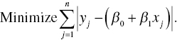
Using Equation (3.1), Boscovich measured the meridian near Rome in 1757. See Stigler (1973) for a detailed description of Equation (3.1). The criterion was the original form of L1 regression, or often referred to as “least absolute value (LAV) regression” in modern statistics and econometrics.
Influenced by Boscovich’s research, Laplace (Pierre Simon Marquis de Laplace: 1749–1827) considered Equation (3.1) to be the best criterion for regression analysis and used it until approximately 1795. At that time, Laplace undertook to serve as a diplomat for Bonaparte Napoleon (1769–1821). However, Laplace thereafter discontinued his examination of the topic because his algorithm for the criterion had a computational difficulty (Eisenhart, 1964).
To describe Laplace’s algorithm for solving Equation (3.1), let us assume that ![]() and
and ![]() ( j = 1, …, n). Then, it is possible for us to reorganize the data set in such a manner that
( j = 1, …, n). Then, it is possible for us to reorganize the data set in such a manner that ![]() . If there is an integer number (ς) that satisfies the following condition:
. If there is an integer number (ς) that satisfies the following condition:
then the estimate of β1 is measured by ![]() 4. A drawback of Laplace’s algorithm is that it can solve only a very small L1 regression problem. Consequently, Laplace stopped studying the L1 regression after 1795 because of the computational difficulty.
4. A drawback of Laplace’s algorithm is that it can solve only a very small L1 regression problem. Consequently, Laplace stopped studying the L1 regression after 1795 because of the computational difficulty.
According to a series of articles prepared by Harter (1974, 1975), the first researcher to overcome the computational difficulty on regression, encountered by Laplace, was Gauss (Carl Friedrich Gauss: 1775–1855). In 1795, when aged only 20, Gauss first proposed the minimization of a sum of squared deviations, which was mathematically expressed by
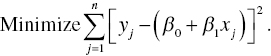
The regression criterion is nowadays referred to as “L2 regression” or “ordinary least squares (OLS)” method. The most important feature of Equation (3.2) is that it is continuous and differentiable. The feature of L2 criterion is different from L1 criterion because the latter is not differentiable and Equation (3.1) needs to be solved as a nonlinear programming problem. Using the L2 criterion, we can easily obtain parameter estimates of a regression line by minimizing Equation (3.2) even if the criterion is applied to a data set with a large sample size. At that time, Gauss believed that the regression criterion was a trivial contribution in science. So, he did not publish the least squares method until 1821. According to Eisenhart (1964), the first researcher who published the method of least squares was Legendre (Adrien Marie Legendre: 1752–1833), who introduced both the regression criterion and the well‐known “least squares normal equations” in 1805.
After the discovery of the least squares method, Gauss studied the probability distribution of errors from 1797 to 1798 and found the “normal distribution.” Gauss proved that least squares estimates became “maximum likelihood estimates” if errors follow the normal distribution. Maximum likelihood estimation was already studied by Daniel Bernoulli (1700–1782) at that time. Unfortunately, Gauss did not publish his findings until 1809. After Gauss published his research results in 1809, Laplace published immediately the “central limit theorem” (Stigler, 1973). Note that the L1 regression produces maximum likelihood estimates under the double exponential distribution, or Laplace distribution. See, for example, the study of Norton (1984).
As a result of the discovery of OLS, normal distribution, normal equations to solve OLS and the central limit theorem, the L2 regression (e.g. least squares method and various extensions) became a main stream of regression analysis in modern statistics and econometrics. The L1 regression had almost disappeared from the history of statistics because of its computational difficulty due to the lack of differentiability as found for the computation of OLS. Most of scientists “religiously” believed that the method of least squares under a normal distribution was the best regression criterion. Even today, none makes any question on the methodological validity of the least squares method. Almost all statistical textbooks at the undergraduate and graduate levels discuss only the least squares method for regression analysis, just neglecting the existence of alternative approaches such as L1 regression5.
The following illustrative example describes differences between L1 regression and L2 regression (i.e., OLS). A supervisor of a manufacturing process believes that an assembly‐line speed (in feet per minute) affects the number of defective parts found during on‐line inspection. To test his belief, management has a uniform batch of parts inspected visually at a variety of line speeds. The data in Table 3.1 are collected for examination.
TABLE 3.1 An illustrative example
| Line speed (feet per minute) | Defective parts (number) |
| 10 | 15 |
| 20 | 25 |
| 30 | 40 |
| 40 | 50 |
| 50 | 75 |
| 60 | 80 |
First, let us consider an estimated regression equation (![]() ) that relates the line speed (x) to the number (y) of defective parts. Using the two estimated equations measured by L1 regression and L2 regression (i.e., OLS), we forecast the number of defective parts found for a line speed of 90 feet per minute. Here, it is not necessary to describe how to apply the L2 regression because it can be easily solved using any statistical code, including Excel. Rather, this chapter documents the following formulation using Equation (3.1):
) that relates the line speed (x) to the number (y) of defective parts. Using the two estimated equations measured by L1 regression and L2 regression (i.e., OLS), we forecast the number of defective parts found for a line speed of 90 feet per minute. Here, it is not necessary to describe how to apply the L2 regression because it can be easily solved using any statistical code, including Excel. Rather, this chapter documents the following formulation using Equation (3.1):

where the above formulation for L1 regression produces an estimated regression line by y = 0.000 + 1.333x, where 0.000 is a very small number close to zero. Meanwhile, L2 regression, or OLS, produces y = –1 + 1.386x. The estimated number of defected parts at the line speed of 90 feet per minute becomes 119.97 under L1 regression and 123.74 under L2 regression. Thus, the two regression analyses have slightly different predictions on the independent variable.
3.3 ORIGIN OF GOAL PROGRAMMING
The computational difficulty related to L1 regression was first overcome by Charnes, Cooper and Ferguson (1955) who transformed the L1 regression into an equivalent linear programming formulation. The computer algorithm for linear programming, referred to as the “simplex method”, was developed in the beginning of 1950s. Along with the development of a computer code using the simplex method at that time, their research first proposed the mathematical formulation for L1 regression.
To describe their reformulation, this chapter generalizes Equation (3.1) in the following vector expression:

where the dependent variable (yj) is to be fitted by a reference to a row vector of m independent variables ![]() for all observations ( j = 1,…,n). The regression model is expressed by Xjβ where
for all observations ( j = 1,…,n). The regression model is expressed by Xjβ where ![]() is a column vector of m + 1 unknown parameters that are to be estimated by Equation (3.3). The superscript (Tr) is a vector transpose.
is a column vector of m + 1 unknown parameters that are to be estimated by Equation (3.3). The superscript (Tr) is a vector transpose.
Following the research effort of Charnes and Cooper (1977), positive and negative parts of each error are introduced to solve Equation (3.3) in the following manner:
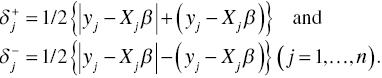
Here, the two equations indicate positive and negative parts of the j‐th error, respectively. Based upon Equations (3.4), the two deviations of the j‐th error become as follows:
Using Equations (3.4) and (3.5), the L1 regression, expressed by Equation (3.3), is reformulated by the following original GP model:

An important feature of Model (3.6)6 is that it can incorporate prior information on parameter estimates into the proposed formulation as additional side constraints. Such an estimation capability cannot be found in conventional regression methods in statistics. For example, Charnes et al. (1955) incorporated such side constraints in order to incorporate hierarchy‐based salary consensus (e.g., the salary of the president is not lower than that of any secretary). See also Sueyoshi and Sekitani (1998a, b) for L1 regression applied to time series analysis that contains serial correlation among different periods.
Model (3.6) is a special case of the GP model7, which incorporates weights (indicating the importance among goals) in the objective function. A weighted GP model can be expressed by

where the j‐th observation on the dependent variable (yj) is replaced by the j‐th goal or objective (obj). Each deviation has a weight (ω) to express the importance of each goal in Model (3.7). The vector β implies not only unknown parameters of a regression model but also other types of unknown decision variables.
The GP terminology was first introduced in Charnes and Cooper (1961) and soon the GP model became widely used as one of the principal methods in the general realm of multi‐objective optimization. See Charnes et al. (1963) and Charnes and Cooper (1975). An important application of the L1 regression can be found in Charnes et al. (1988) that was an extension of their previous works (e.g., Charnes et al., 1986). Their research in 1988 discussed the existence of a methodological bias in empirical studies. The methodological bias implies that “different methods often produce different results.” It is necessary for us to examine different methods to make any suggestion for large decisional issues. The research concern is very important in particular when we make a policy suggestion from empirical evidence for guiding large policy issues such as global warming and climate change. A few previous studies have mentioned an existence of the methodological bias in energy and environmental studies.
Hereafter, let us discuss how to apply Model (3.6) for GP by using an illustrative example. The example is summarized as follows: There are many leaking tanks in gas stations which often reach underground water sources and produce serious water pollution. An environmental agency needs to replace old leaking tanks by new ones. As an initial step, the agency attempts to determine its location in the area covered by existing four gas stations to be fixed. Using horizontal and vertical coordinates, the gas stations containing leaking tanks are located at (1,7), (5, 9), (6, 25) and (10, 20).
To solve the problem by GP, let β be (hc, vc)Tr where hc and vc stand for unknown decision variables that indicate the location of agent’s office in horizontal and vertical coordinates, respectively. The GP model is formulated as follows:

where all weights (ωj) are set to be unity because all goals are equally important in the location problem.
The optimal solution of the above GP problem is hc* = 6 and vc* = 20. In other words, the best location of the agent is (6, 20) on the horizontal and vertical coordinates. This chapter needs to note two concerns on the optimal solution. One of the two concerns is that both hc and vc are non‐negative, as formulated above, because the GP formulation is for a locational problem, not the regression analysis as discussed previously. The other concern is that the optimal solution may suffer from an occurrence of multiple solutions. This type of difficulty often occurs because the problem is formulated and solved by linear programming.
3.4 ANALYTICAL PROPERTIES OF L1 REGRESSION
Returning to Model (3.6) for L1 regression, this chapter discusses the dual formulation and the implication of dual variables. First, Model (3.6) is reorganized by the following GP model for L1 regression that is more specific than the original formulation:

Here, it is important to reconfirm that β0 is an unknown parameter to express the constant of a regression model and βi (i = 1,…,m) are unknown parameters to be estimated. They indicate the slope of the regression model ![]() . The subscript (j) stands for the j‐th observation.
. The subscript (j) stands for the j‐th observation.
The dual formulation of Model (3.8) becomes
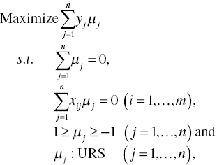
where μj stands for the dual variable for the j‐th observation. The complementary slackness conditions, that is, ![]() and
and ![]() for all j, of linear programming indicates the following relationship between Models (3.8) and (3.9):
for all j, of linear programming indicates the following relationship between Models (3.8) and (3.9):
if ![]() , then
, then ![]() (the j‐th observation locates above the regression hyperplane),
(the j‐th observation locates above the regression hyperplane),
if ![]() , then
, then ![]() (the j‐th observation locates on the regression hyperplane) and
(the j‐th observation locates on the regression hyperplane) and
if ![]() , then
, then ![]() (the j‐th observation locates below the regression hyperplane).
(the j‐th observation locates below the regression hyperplane).
Thus, the optimal dual variable (![]() ) related to the j‐th observation describes the locational relationship between an estimated regression hyperplane and the observation.
) related to the j‐th observation describes the locational relationship between an estimated regression hyperplane and the observation.
Following the research of Sueyoshi and Chang (1989), this chapter may obtain an interesting transformation that changes the j‐th dual variable by ![]() . Then, Model (3.9) becomes
. Then, Model (3.9) becomes

Model (3.10) is equivalent to the following formulation:
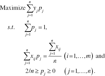
An important feature of Model (3.11) is that the dual variable (pj) for the j‐th observation may be considered as a “probability” that the observation locates above an estimated regression hyperplane. In other words,
- if pj = 2/n, then the observation locates above the regression hyperplane,
- if 2/n >pj> 0, then it locates on the hyperplane and
- if pj = 0, then it locates below the regression hyperplane.
3.5 FROM L1 REGRESSION TO L2 REGRESSION AND FRONTIER ANALYSIS
3.5.1 L2 Regression
This chapter can reorganize Model (3.2), as an extension of Model (3.8), by slightly changing the objective function as follows:

The difference between Models (3.8) and (3.12) is that the objective function of the latter model minimizes the sum of squared errors, measured by slacks, so that it corresponds to the OLS. One problem is that Model (3.12) belongs to nonlinear programming so that it may have limited computational practicality. The contribution of Gauss in the eighteenth century was that he solved Model (3.12) by a matrix operation so that his approach could deal with a large data set for regression analysis, as mentioned previously.
3.5.2 L1‐Based Frontier Analyses
Another important extension of Model (3.8) is that it is possible for us to use it for frontier analysis, which is closely related to DEA, along with minor modifications. There are two alternatives for frontier analysis. One of the two alternatives is for production analysis that is formulated as follows:

Model (3.13) produces an estimated (lower) regression hyperplane that locates on or below all the observations. One‐sided slacks (![]() ) are considered in the objective function of Model (3.13). This type of frontier analysis is useful for estimating a cost function.
) are considered in the objective function of Model (3.13). This type of frontier analysis is useful for estimating a cost function.
The other alternative is formulated as follows:

Model (3.14) indicates an opposite case to that of Model (3.13). One‐sided slacks (![]() ) are considered in the objective function of Model (3.14). An estimated (upper) regression hyperplane locates on or above all the observations. This type of frontier analysis is useful for estimating a production function.
) are considered in the objective function of Model (3.14). An estimated (upper) regression hyperplane locates on or above all the observations. This type of frontier analysis is useful for estimating a production function.
Methodological strengths and drawbacks of Models (3.13) and (3.14), compared with DEA, are summarized as the following four differences: First, Models (3.13) and (3.14) can be used for efficiency assessment that compares observations by two estimated frontiers, respectively. Functionally, the proposed frontier analyses work like DEA in their efficiency assessments. Second, these models can directly handle zero and/or negative values in a data set. A problem is that the frontier analyses measure the performance of observations by only a single desirable output. In contrast, DEA can handle multiple desirable outputs, but it cannot directly handle zero and/or negative values. See Chapters 26 and 27 for a description on how to handle zero and/or negative values by DEA and its environmental assessment. Third, another difference between DEA and the frontier analyses is that DEA can avoid specifying a functional form. In contrast, the frontier analysis requires the functional specification. Finally, both L1‐based frontier analyses and DEA can evaluate the performance of observations (i.e., DMUs). The L1‐based frontier analyses look for parameter estimates of two frontier hyperplanes, while DEA measures weights on production factors (i.e., inputs and desirable outputs). That is a structural difference between L1‐based frontier analyses and DEA.
Table 3.2 lists an illustrative example for L1‐based frontier analyses. The data set contains ten observations (DMUs), each of which has an independent variable (x) and a dependent variable (y). Figure 3.1 compares three regression lines which are estimated by L1 regression and two L1‐based frontier analyses, respectively. The L1 regression is measured by Model (3.8). The two frontier analyses are measured by Models (3.13) and (3.14), respectively. Model (3.8) estimates L1 regression line as y = 6 + 0.75x. Models (3.13) and (3.14) estimate the two L1‐based frontier lines as y = –1.5 + 1.375x (as a lower bound) and y = 9.286 + 0.571x (as an upper bound), respectively.
TABLE 3.2 An illustrative example for L1 frontier analyses
| Observation | x | y |
| 1 | 10 | 15 |
| 2 | 3 | 11 |
| 3 | 5 | 10 |
| 4 | 2 | 6 |
| 5 | 4 | 9 |
| 6 | 4 | 4 |
| 7 | 12 | 15 |
| 8 | 7 | 13 |
| 9 | 6 | 8 |
| 10 | 8 | 12 |

FIGURE 3.1 Three regression lines: L1 regression and two frontier analyses (a) Each dot (•) indicates an observation. (b) The L1 regression, locating in the middle of observations, is measured by Model (3.8). The L1‐based lower frontier line is measured by Model (3.13) and the L1‐based upper frontier line is measured by Model (3.14).
Table 3.3 summarizes upper and lower estimates determined by the two L1‐based frontier analyses. The upper estimates are listed in the fourth row of Table 3.3 and the corresponding efficiency scores are measured by ![]() , where yj is the observed dependent variable of the j‐th DMU and
, where yj is the observed dependent variable of the j‐th DMU and ![]() is its upper estimate of the j‐th observation. The lower estimates and efficiency scores are listed in the bottom of Table 3.3. The efficiency scores are measured by
is its upper estimate of the j‐th observation. The lower estimates and efficiency scores are listed in the bottom of Table 3.3. The efficiency scores are measured by ![]() where
where ![]() is the lower estimate of the j‐th observation.
is the lower estimate of the j‐th observation.
TABLE 3.3 Efficiency measures by L1‐based Frontier analyses
| DMU | 1 | 2 | 3 | 4 | 5 | 6 | 7 | 8 | 9 | 10 |
| x | 10 | 3 | 5 | 2 | 4 | 4 | 12 | 7 | 6 | 8 |
| y | 15 | 11 | 10 | 6 | 9 | 4 | 15 | 13 | 8 | 12 |
| Upper Estimate | 15.00 | 11.00 | 12.14 | 10.43 | 11.57 | 11.57 | 16.14 | 13.28 | 12.71 | 13.85 |
| Efficiency | 1.00 | 1.00 | 0.82 | 0.58 | 0.78 | 0.35 | 0.93 | 0.98 | 0.63 | 0.87 |
| Lower Estimate | 12.25 | 2.63 | 5.38 | 1.25 | 4.00 | 4.00 | 15.00 | 8.13 | 6.75 | 9.50 |
| Efficiency | 0.82 | 0.24 | 0.54 | 0.21 | 0.44 | 1.00 | 1.00 | 0.63 | 0.84 | 0.79 |
It is necessary to add two concerns on the L1 regression and two L1‐based frontier analyses. One of the two concerns is that, as found in Figure 3.1 and Table 3.3, these methodologies need multiple constraints to identify an optimal solution by linear programming formulations. See Models (3.12) to (3.14) in which each observation corresponds to each constraint in these formulations. The optimality is found on a “vertex” that consists of multiple (e.g., at least two) constraints. Each vertex is a corner point in a feasible region of linear programming. Thus, the vertex on optimality needs multiple constraints, so multiple observations. See, for example, Figure 3.1 in which each line passes on two observations. See also Table 3.3 in which two observations are efficient in upper and lower estimates. Later in this book, we will discuss that DEA suffers from an occurrence of multiple efficient (often many) organizations because of the same mathematical reason.
The unique feature indicates a methodological drawback, but simultaneously implying a methodological strength. That is, L1 regression hyperplane estimated by Model (3.8) is robust to an existence of an outlier. In a similar manner, the upper frontier hyperplane estimated by Model (3.13) is robust to an outlier locating below the frontier. An opposite case can be found in the lower frontier hyperplane estimated by Model (3.14). It is indeed true that the unique feature is a methodological strength. However, if the two observations on an estimated regression line do not indicate the direction of an observational sample, then the proposed three models may not produce reliable estimates on the three regression hyperplanes. That indicates a methodological drawback of the L1 regression and two L1‐based frontier analyses.
In applying regression to various decisional issues, we need to use a functional form (e.g, Cobb–Douglas and translog functions) in Models (3.13) and (3.14) if a repression hyperplane is expressed by a linear relationship. See, for example, Charnes et al. (1988), Sueyoshi (1991) and Sueyoshi (1996) that discussed the importance of selecting different combinations of L1 or L2 regression method, regression analysis or frontier analysis, along with a selection of various functional forms, for guiding large public policy issues (e.g, the divestiture of a telecommunication industry in industrial nations such as the United States and Japan). Their concern is still useful and important in most current empirical studies. That it, it is necessary for researchers to examine different methodology combinations (i.e., regression vs frontier, L1 vs L2 and various functional forms) in order to avoid a methodological bias on empirical studies in energy and environment. It is indeed true that the L2 regression is very important and widely used by many studies, but it is only one of many regression analyses. It is also necessary for us to understand that there is no perfect methodology. Hence, we constantly make an effort to improve the quality of our methodology, looking for methodological betterment, until we can guide various policy and strategic issues by providing reliable empirical evidence.
3.6 ORIGIN OF DEA
The GP served as a methodological basis for the development of DEA with a linkage via “fractional programming” (Charnes and Cooper, 1962, 1973). The reformulation from a fractional model8 to a linear programming equivalence was first proposed by Charnes et al. (1978, 1981) and the reformulation was widely used in the OR and MS literature. The reformulation was also used to develop the first DEA model, often referred to as a “ratio form,” because of the relationship to fractional programming as discussed in Chapter 2. See also Chapter 1 for a description on DEA. See also Figure 3.2.

FIGURE 3.2 Progress from L1 regression to DEA.
(a) Source: Glover and Sueyoshi (2009)
The ratio form (for input‐oriented measurement) has the following formulation to determine the level of efficiency9 on the k‐th organization:

Model (3.15) evaluates the performance of the k‐th organization by relatively comparing it with those of n organizations (j = 1,…,n) in relation to each other. Hereafter, each organization, referred to as a decision making unit (DMU) in DEA, uses m inputs (i = 1,…,m) to produce s desirable outputs (r = 1,…,s). The xij is an observed value related to the i‐th input of the j‐th DMU and the grj is an observed value related to its r‐th desirable output. Slacks (i.e., deviations) related to inputs and desirable outputs are ![]() and
and ![]() , respectively. The symbol (εn) stands for a non‐Archimedean small number. The scalar (λj), often referred to as a “structural” or “intensity” variable, is used to make a linkage among DMUs in a data domain of inputs and desirable outputs. An efficiency score is measured by an unknown variable (θ) that is unrestricted in Model (3.15). The status of operational efficiency is confirmed by Model (3.15) when both
, respectively. The symbol (εn) stands for a non‐Archimedean small number. The scalar (λj), often referred to as a “structural” or “intensity” variable, is used to make a linkage among DMUs in a data domain of inputs and desirable outputs. An efficiency score is measured by an unknown variable (θ) that is unrestricted in Model (3.15). The status of operational efficiency is confirmed by Model (3.15) when both ![]() and all slacks are zero on optimality, as discussed in Chapter 2. An important feature of Model (3.15), to be noted here, is that it is input‐oriented. It is possible for us to change Model (3.15) into a desirable output‐oriented formulation.
and all slacks are zero on optimality, as discussed in Chapter 2. An important feature of Model (3.15), to be noted here, is that it is input‐oriented. It is possible for us to change Model (3.15) into a desirable output‐oriented formulation.
At the end of this section, we need to mention that Chapter 2 does not incorporate the non‐Archimedean small number (εn) because of our descriptive convenience. However, this chapter incorporates the very small number in the DEA formulation. It is true that if we are interested in measuring only the level of efficiency, then the incorporation may not produce a major influence on the magnitude of efficiency. Furthermore, the non‐Archimedean small number is just our mathematical convenience in the context of production economics. In reality, none knows what it is.
Clearly acknowledging such concerns on εn, this chapter needs to mention the two other analytical concerns. One of the two concerns is that if we drop εn in the objective function, then dual variables (multipliers) often become zero in these magnitudes. This is problematic because the result clearly implies that corresponding inputs or desirable outputs are not utilized in DEA assessment. The other concern is that if we are interested in not only an efficiency level but also other types of measurement (e.g., marginal rate of transformation and rate of substitution), then dual variables (multipliers) should be strictly positive in these signs. Otherwise, the computational results obtained from DEA are often useless, so not conveying any practical implications to users. Thus, the incorporation of such a very small number is important for DEA as first proposed in the original ratio model (Charnes et al., 1978, 1981) at this stage. See Chapters 23, 26 and 27 for detailed discussions on various DEA problems due to an occurrence of zero in dual variables.
3.7 RELATIONSHIPS BETWEEN GP AND DEA
DEA researchers have long paid attention to the additive model, first proposed by Charnes et al. (1985), because it has the analytical structure based upon Pareto optimality. See Chapter 5 for a detailed description on the additive model. Although Chapter 2 does not clearly mention it, Model (2.7) belongs to the additive model that is designed to identify the total amount of slack(s) on optimality. See also the research of Cooper et al. (2006) that discussed the relationship between the ratio form and the additive model. An important feature of the additive model is that it aggregates input‐oriented and desirable output‐oriented measures to produce a single measure for operational efficiency (OE). Acknowledging that Cooper (2005) has already discussed the relationship between GP and the additive model, this chapter does not follow his description, rather it discusses another path to describe the differences between them.
First of all, it is important for us to confirm that the efficiency of the k‐th DMU is measured by the following additive model:

Since Model (3.16) does not have any efficiency score (θ), as found in Model (3.15), it measures a level of OE by the total amount of slacks. The status of efficiency is measured as follows:
- Full efficiency ↔ all slacks are zero and
- Inefficiency ↔ at least one slack is non‐zero.
See Chapters 5 and 6 that provide detailed descriptions on the additive model.
To discuss an analytical linkage between the additive model and the GP, this chapter returns to Models (3.13) and (3.14) as special cases of GP. This chapter considers the following four steps to identify such an analytical linkage between them:
- Step 1 (objective change from minimization to maximization): The frontier analysis models, or Models (3.13) and (3.14), are reorganized as follows:andwhere we change the objective function from minimization to maximization in Models (3.13) and (3.14). Accordingly, the sign of slacks (
 ) is changed from negative to positive in Model (3.17). In contrast, the sign of slacks (
 ) is changed from positive to negative in Model (3.18). Thus, the combination between Models (3.13) and (3.14) is equivalent to that of Models (3.17) and (3.18). However, the relationship between lower and upper bounds in the former models becomes opposite in the latter models.
 - Step 2 (from parameters to weights): The purpose of the two frontier analyses models is to determine the upper and lower frontier hyperplanes, both of which connect these parameter estimates, because they belong to regression analysis. In contrast, the purpose of the additive model is to identify an efficiency frontier that consists of inputs and desirable outputs regarding n DMUs (so, being observations) and to determine the level of their efficiency scores by the total sum of slacks. Therefore, we set
 (so, no constant) in Models (3.17) and (3.18) and then replace the unknown parameters (βi for i = 1,..., m) in Models (3.17) and (3.18) by other unknown intensity variables (λj for j = 1,…, n). In this case, it is necessary to exchange j = 1,..., n and r = 1,…, s in Model (3.17) as well as j = 1,…, n and i = 1,..., m in Model (3.18).
 - Step 3 (from dependent variables to inputs and desirable outputs on the k‐th DMU): We incorporate two different groups into Models (3.17) and (3.18) to obtain GP formulations. One of the two groups (for desirable outputs) has s goals (grk: r = 1,…, s) of the k‐th DMU to replace yj ( j = 1,…, n) in Model (3.17). The other group (for inputs) has m goals (xik: i = 1,…, m) of the k‐th DMU to replace yj ( j = 1,…, n) in Model (3.18). Furthermore, an input‐oriented frontier is less than or equal xik. In contrast, a desirable output‐oriented frontier is more than or equal grk. By paying attention to these analytical features, this chapter reorganizes Models (3.17) and (3.18) as follows: and
Here, the observation (j) in Model (3.17) is replaced by the goal (r) so that Equation (3.19) has
 on the left hand side. In a similar manner, the observation (j) in Model (3.18) is replaced by the goal (m) so that Model (3.20) has
  on the left hand side.
 - Step 4 (normalization): We combine Models (3.19) and (3.20) and then incorporates the condition for “normalization” on unknown intensity variables (i.e.,
 ) in the combined formulation. The normalization makes it possible that parameters estimates of regression are changed to weights among production factors as formulated in DEA. As a result of such a combination, we can obtain the formulation of Model (3.16).


3.8 HISTORICAL PROGRESS FROM L1 REGRESSION TO DEA
Figure 3.2 visually describes the historical development flow from L1 regression to DEA. The figure reorganizes the part of Professor Cooper’s view on DEA development, as depicted in the upper part of Figure 1.1. This chapter specifies it more clearly in such a manner that it can fit within the context of this book.
3.9 SUMMARY
The first publication of DEA was generally regarded as the article prepared by Charnes et al. (1978) although Professor Cooper and his associates presented DEA at the TIMS Hawaii conference in 1977. Viewing DEA as an extension of GP, along with fractional programming and in consideration of the historical linkage between L1 regression and GP, this book considers that DEA has an analytical linkage with L1 regression. In this concern, the history of DEA was connected in a roundabout fashion with developments of science in the eighteenth century, as manifested in the work of Laplace and Gauss, because they attempted to develop algorithms for the L1 regression. That was the view on the DEA development of Professor Cooper.
Following Professor Cooper’s view on GP and DEA, which has been never documented in his previous publications, this chapter has reviewed these historical linkages. For example, DEA has many methodological benefits as a non‐parametric approach10 that does not assume any functional form on specification between inputs and desirable outputs. Furthermore, DEA can be solved by linear programming. The computational tractability attracts many users in assessing performance of organizations in private and public sectors. However, it may be true that DEA has often misguided many previous applications. To avoid the misuse found in many previous research efforts, it is necessary for us to pay attention to a careful examination on unique features of DEA performance analysis. As an extension of a conventional use of DEA, the environmental assessment, which is the main research concern of this book, we will discuss methodological benefits and drawbacks of DEA from the perspective of environmental assessment in Section II.