
5
NON‐RADIAL MEASUREMENT
5.1 INTRODUCTION
This chapter1 discusses non‐radial models based upon the Pareto–Koopmans measurement to determine the level of operational efficiency (OE). The DEA assessment is generally separated into two groups of models. One of the two groups is referred to as “radial measures,” or input and desirable output‐oriented RM(v) and RM(c), as discussed in Chapter 4. The other group of models includes “non‐radial measures,” most of which are discussed in this chapter. The radial models, belonging to “Debreu–Farrell measures,” can determine the level of OE regarding DMUs by examining an efficiency score, along with slacks, in the objective function of their linear programming formulations2. In contrast, the non‐radial measures (e.g., an additive model: Charnes et al., 1985), discussed in this chapter determine the OE level by examining the total amount of slacks, because they do not have any efficiency score in these objective functions. This type of measure belongs to the “Pareto–Koopmans measure” (Koopmans, 1951; Russell, 1985).
In addition to these OE measurement criteria, it is important to note that the proposed non‐radial measures can avoid specifying the non‐Archimedean small number (εn). The unique feature is important because none knows what it is in reality. See Chapter 7 for a discussion on another approach to avoid specifying such a small number even in the radial measures.
This chapter is concerned with descriptions on five non‐radial models in terms of their OE assessments. Section 5.2 compares analytical differences between the Debreu–Farrell type of radial models and the Pareto–Koopmans type of non‐radial models from the perspective of OE as well as characterization and classifications of DMUs. This type of comparison has been not sufficiently explored in previous studies on radial and non‐radial comparison. The proposed comparison provides us with unique features of non‐radial models and their implications in DEA. Section 5.3 discusses the “Russell measure” which provides us with a theoretical linkage between radial and non‐radial measurements. An important feature of the Russell measure is that it is formulated by non‐linear programming because it can unify input‐oriented and desirable output‐oriented measures. As a consequence of the non‐linear programming structure, the Russell measure has a computational difficulty although it has indeed several desirable properties as an OE measure, all of which may not be found in radial models. Section 5.4 discusses “an additive model” as the second non‐radial model, proposed by Charnes et al. (1985). Charnes et al. (1982, 1983) linked the additive model to “a multiplicative model,” as the third non‐radial measure, by changing a data set by a natural logarithm. This chapter considers that the two non‐radial models (additive and multiplicative) are same because a difference can be found in only the data manipulation. Section 5.5 discusses “a range‐adjusted measure (RAM)” as the fourth non‐radial model. Cooper et al. (1999) proposed the RAM as an extension of the additive model (Cooper et al., 2000, 2001). Section 5.6 investigates slack‐adjusted radial measure (SARM) as an extension of RAM, serving as the fifth alternative. Although the DEA community did not pay serious attention to SARM, the model will serve as a methodological basis for DEA environmental assessment in Section II. Tone (2001) proposed another type of non‐radial model, referred to as slack‐based measure (SBM) as the sixth non‐radial model. SBM is discussed in Section 5.7. Section 5.8 prepares methodological comparison among radial and non‐radial models for the conventional use of DEA. Section 5.9 summarizes this chapter.
At the end of this section, we clearly acknowledge that there are many other types of model variations related to non‐radial measurement. Most of them are originated from the radial and non‐radial models examined in Chapter 4 and this chapter. Unfortunately, this chapter cannot cover all of them because the purpose of this book is the DEA environmental assessment of energy and sustainability. The approach is conceptually and analytically different from a conventional use of DEA as discussed in the chapters of Section II. However, our description in this chapter provides us with an analytical basis on how to extend DEA to the proposed energy and environmental assessment.
5.2 CHARACTERIZATION AND CLASSIFICATION ON DMUs
This chapter characterizes analytical differences between the Debreu–Farrell (for radial) and Pareto–Koopmans (for non‐radial) types of efficiency measures from DEA solutions and then classifies all DMUs based upon the characterization. A description on such distinctions is also discussed from economic and analytical linkages with the concept of Pareto optimality because it provides DEA with a theoretical basis for relative efficiency measurements and algorithm developments for non‐radial measurement. See Chapter 10, which fully utilizes the characterization and classification of DMUs for algorithmic development on network computing.
In this chapter, we interpret the concept of Pareto optimality as follows: “Pareto Optimality: There is no other DMU which outperforms a specific DMU in terms of all components of production factors without changing the structure of an efficiency frontier.”
According to today’s global economy (https://www.britannica.com/topic/Pareto‐optimality), the original definition of Pareto optimality is different from the above. This chapter interprets the optimality concept from a perspective of DEA performance assessment. An important contribution of Pareto optimality in this chapter is that it provides DEA with an underlying definition of relative efficiency. Koopmans (1951) used the concept to connect between inputs and desirable outputs and apply it for measuring productivity and other efficiencies. As a consequence, the efficiency measures based upon Pareto optimality are referred to as “Pareto–Koopmans” measures (or non‐radial measures) in this chapter.
To prepare an analytical linkage between the concept of Pareto optimality and the status of OE, this chapter starts discussing the DMU characterization and classification first proposed by Charnes et al. (1986, 1991). As mentioned above, the classification has been extended into the development of special computer algorithms which can solve various radial and non‐radial DEA models. See Chapter 10.
An important condition derived from the Pareto optimality is a concept of “dominance” that is often utilized for DEA algorithmic developments. The concept is specified as follows:
Dominance:
The DMU classification (e.g., Sueyoshi, 1990; Sueyoshi and Chang, 1989) partitions a whole set (J) of all DMUs into two subsets: ![]() . One subset (Jd) is a dominated set and the other (Jn) is a non‐dominated set. To specify the two groups, a concept of dominance is mathematically specified by:
. One subset (Jd) is a dominated set and the other (Jn) is a non‐dominated set. To specify the two groups, a concept of dominance is mathematically specified by:
Here, “![]() ” implies that at least one component of the two vectors of production factors has the relationship “>.” The production factors are expressed by input and desirable output vectors as specified by the two parts of Equation (5.1), respectively. Using Equation (5.1), the two subsets become as follows:
” implies that at least one component of the two vectors of production factors has the relationship “>.” The production factors are expressed by input and desirable output vectors as specified by the two parts of Equation (5.1), respectively. Using Equation (5.1), the two subsets become as follows:
The concept of dominance is closely related to the Pareto optimality because DMUs, which are on the Pareto optimality, comprise the members of Jn. The opposite is not true. As a result, it is important for DEA to eliminate Jd from an efficiency frontier at the early stage of DEA computation. An algorithm for DEA needs to pay attention to only DMUs in Jn before the computational process of the whole DMUs.
In the case of Pareto–Koopmans (non‐radial) measures (e.g., an additive model and RAM), the two subsets are further separated in the following manner (e.g., Sueyoshi and Chang, 1989):
where the four subsets are defined by the following specifications:
The symbols “![]() ” and “
” and “![]() ” means “all” and “some,” respectively. In the above classification, efficient DMUs (
” means “all” and “some,” respectively. In the above classification, efficient DMUs (![]() ) attain the status of Pareto optimality, but inefficient DMUs (
) attain the status of Pareto optimality, but inefficient DMUs (![]() : not clearly inefficient and
: not clearly inefficient and ![]() : clearly inefficient) do not belong to the optimality status.
: clearly inefficient) do not belong to the optimality status.
Meanwhile, the Debreu–Farrell (radial) measures such as RM(v) and RM(c) may separate the whole data set into the following six subsets (e.g., Sueyoshi, 1992):
all of which may be redefined by the following six subsets:
The proposed two groups of DMU classifications, that is, Equations (5.3) and (5.4), indicate five important concerns to be discussed here. First, multiple solutions occur on DMUs belonging to E '. Second, the Debreu–Farrell (radial) measures have IF and IF′, while the Pareto–Koopmans (non‐radial) measures do not have such two subsets because the Pareto optimality excludes them from an efficiency frontier. Such a difference indicates that the computational process for Pareto–Koopmans measures is more tractable and faster than that of Debreu–Farrell measures because the former group consists of only four DMU classifications. Third, the concept of Pareto optimality makes it possible that we measure the level of OE by examining a total amount of slacks on optimality. Fourth, both the Debreu–Farrell (radial) and Pareto–Koopmans (non‐radial) measures have inefficient DMU group (IE ') whose status is not clearly identified by the concept of dominance (non‐dominated but not Pareto optimal). Finally, it is easily imagined that we can effectively solve the whole DMU set by identifying efficient DMUs and eliminating inefficient DMUs at the early stage of DEA computation. The algorithm development, incorporating the Pareto optimality and the concept of dominance, will be discussed in Chapter 10.
5.3 RUSSELL MEASURE
Maintaining the unique features of both radial and non‐radial measures, the Russell measure determines a level of OE by aggregating the efficiency scores related to all production factors (Russell, 1985):
The Russell measure on the k‐th DMU is measured by the following formulation:

where unknown variables (θi and τr) indicate the level of each OE measure related to the i‐th input (i = 1,…, m) and the r‐th desirable output (r = 1,…, s), respectively. It is possible to incorporate slacks in Model (5.5). This chapter follows the original description prepared by Russell (1985), so not incorporating slacks in Model (5.5).
An important feature of Model (5.5) is that it is formulated by non‐linear programming, as found in the objective function of Model (5.5). Sueyoshi and Sekitani (2007b) have proposed a use of “second‐order cone programming (SOCP),” which is a new optimization approach originated from an interior point method of linear and non‐linear programming, both to compute directly the Russell measure and to obtain the dual formulation. The SOCP approach proposed by their study can provide an exact solution on the Russell measure. Since we do not use the Russell measure for DEA environmental assessment in Section II, this chapter does not describe it further, except noting that interesting readers may refer to the research effort in the following: Sueyoshi and Sekitani (2007b), Computational strategy for Russell measure in DEA: Second‐order cone programming. European Journal of Operational Research, 180, 459–471.
It can be easily imagined that an extension of Model (5.5) to DEA environmental assessment is a straightforward matter with a minor modification on SOCP.
To solve Model (5.5) by an approximation (short‐cut) approach, Bardhan et al. (1996a, b) reformulated it as a linear programming problem. The Russell measure approximation may be expressed by the following input‐oriented model on the k‐th DMU:

The original Russell measure is formulated under constant RTS because it does not contain the side constraint ![]() . It is possible for us to incorporate the side constraint into Models (5.5) and (5.6), so reformulating it under variable RTS.
. It is possible for us to incorporate the side constraint into Models (5.5) and (5.6), so reformulating it under variable RTS.
The Russell measure aggregates all efficiency scores (θi) related to all inputs (i = 1,…, m). Hence, Models (5.5) and (5.6) do not belong to the conventional radial measurement, rather expressing the magnitude of each individual efficiency score in so‐called “Pareto improvement” on a specific production factor. In the implication, this chapter considers that the Russell measure exists between the radial measure (indicating the improvement of all production factors) and non‐radial measure (indicating the improvement on each production factor). On the optimality of Model (5.6), where we can obtain ![]() (i = 1,…, m) and
(i = 1,…, m) and ![]() (j = 1,…, n), the input‐based Russell measure (Russellin) on the k‐th DMU is determined by
(j = 1,…, n), the input‐based Russell measure (Russellin) on the k‐th DMU is determined by

where ![]() is obtained from the optimality of Model (5.6). Equation (5.7) measures an average of the aggregated input‐oriented efficiency scores.
is obtained from the optimality of Model (5.6). Equation (5.7) measures an average of the aggregated input‐oriented efficiency scores.
Shifting from the input‐oriented measurement, an approximation approach for the Russell measure becomes the following desirable output‐oriented model on the k‐th DMU:

Model (5.8) is formulated by maximizing the total sum of efficiency scores (τr) on all desirable outputs. On the optimality of Model (5.8), where we can obtain ![]() (r = 1,…, s) and
(r = 1,…, s) and ![]() (j = 1,…, n), the desirable output‐based Russell measure (Russellout) concerning the k‐th DMU is determined by
(j = 1,…, n), the desirable output‐based Russell measure (Russellout) concerning the k‐th DMU is determined by

An important feature of the proposed Russell measure is that it aggregates the desirable output‐oriented measures and Equation (5.9) measures an average of these efficiency scores.
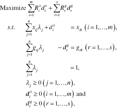
According to Bardhan et al. (1996a,b), the combined formulation between inputs and desirable outputs becomes as follows:

Model (5.10) has positive on the first term and negative on the second term of the objective function because the inputs are minimized while the desirable outputs are maximized in the Russell measurement. The negative sign in minimization implies maximization in the objective function. Thus, the part ![]() in the objective function of Model (5.10) substitutes for the part
in the objective function of Model (5.10) substitutes for the part 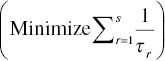 of Model (5.5).
After obtaining ![]() (i = 1, …, m) and
(i = 1, …, m) and ![]() (r = 1, …, s) on the optimality of Model (5.10), this chapter can determine the Russell measure (Russellboth) for inputs and desirable outputs as follows:
(r = 1, …, s) on the optimality of Model (5.10), this chapter can determine the Russell measure (Russellboth) for inputs and desirable outputs as follows:

On the optimality of Equation (5.11), the k‐th DMU satisfies the following conditions on an efficiency frontier:

Equations (5.12) implies that all the slacks are zero. The Russell measure determines a level of improvement on each production factor and obtains an average regarding those of all production factors. Thus, the Russell measure contains such a non‐radial property, so that we can consider as an intermediate model between radial and non‐radial measurements.
5.4 ADDITIVE MODEL
DEA researchers have long paid attention to the additive model (AM) as an alternative to the two radial models, because the non‐radial model aggregates input‐oriented and desirable output‐oriented measures to produce a single non‐radial measure for OE. The AM is mathematically specified as follows:

The objective value indicates the level of inefficiency measured by an amount of total slacks related to all inputs and desirable outputs.
The level of OE, or AM efficiency, regarding the k‐th DMU is determined by

where the slack values ![]() and
and ![]() are determined on the optimality of Model (5.13).
are determined on the optimality of Model (5.13).
In addition to Model (5.13), it is possible for us to change the objective function by adding weights (![]() and
and ![]() ) to slacks in the objective function of Model (5.13) in order to control the magnitude of inefficiency. The weights are also used to express the importance among inputs and desirable outputs. In the case, the objective function of Model (5.13) becomes as follows:
) to slacks in the objective function of Model (5.13) in order to control the magnitude of inefficiency. The weights are also used to express the importance among inputs and desirable outputs. In the case, the objective function of Model (5.13) becomes as follows:

A practical difficulty of the AM with the objective function, expressed by Equation (5.15), is that none knows how to determine such weights in the objective function. Cooper et al. (1999) proposed measuring the OE of the k‐th DMU after changing ![]() and
and ![]() in Equation (5.15). This type of adjustment is later referred to as a range‐adjusted measure (RAM). The adjustment method is one of many alternatives for weight selection in Equation (5.15). The level of OE of the k‐th DMU is determined by
in Equation (5.15). This type of adjustment is later referred to as a range‐adjusted measure (RAM). The adjustment method is one of many alternatives for weight selection in Equation (5.15). The level of OE of the k‐th DMU is determined by

where the slack values ![]() and
and ![]() are obtained from the optimality of Model (5.13) which is adjusted by Equation (5.15) with
are obtained from the optimality of Model (5.13) which is adjusted by Equation (5.15) with ![]() and
and ![]() . Each slack is divided by the corresponding observed input or desirable output and the total number of inputs and desirable outputs. Consequently, the second part of the right hand side of Equation (5.16) indicates a level of total inefficiency. The AM efficiency is determined by subtracting the total inefficiency from unity.
. Each slack is divided by the corresponding observed input or desirable output and the total number of inputs and desirable outputs. Consequently, the second part of the right hand side of Equation (5.16) indicates a level of total inefficiency. The AM efficiency is determined by subtracting the total inefficiency from unity.
The efficiency status of AM is classified into the following two cases: (a) AM efficiency ↔ all slacks are zero and (b) AM inefficiency ↔ at least one slack is positive on optimality.
Multiplicative Model:
If a data set on inputs and desirable outputs is expressed by natural logarithm, the additive model is referred to as “a multiplicative model” that corresponds to a generalization of Cobb‐Douglas type of production functions (Cooper et al., 1982, 1983; Sueyoshi and Chang, 1989). Mathematically, the model changes a data set (xij, grj) to ![]() , where
, where ![]() and
and ![]() for all i and all r of the j‐th DMU (j = 1,…, n). Thus, the inputs and desirable outputs have the Cobb–Douglas type of relationships such as
for all i and all r of the j‐th DMU (j = 1,…, n). Thus, the inputs and desirable outputs have the Cobb–Douglas type of relationships such as ![]() and
and ![]() . Model (5.13) for the multiplicative model becomes as follows:
. Model (5.13) for the multiplicative model becomes as follows:

Here, it is important to note three concerns on Model (5.17). First, the multiplicative model is the same as the additive model in (5.13) except the data transformation by natural logarithm. Therefore, this chapter considers that there is no difference between the additive model and the multiplicative model. Second, the multiplicative model requires that all inputs and desirable outputs are strictly positive because of the data logarithmic transformation. The property on data is required on not only the multiplicative model but also all DEA models. See Chapters 26 and 27 for a description on how to handle zero and negative values in a data set. Finally, Cooper et al. (2006, p. 114) documented the multiplicative model under constant RTS by dropping ![]() from Model (5.17). The model adds the side constraint under variable RTS.
from Model (5.17). The model adds the side constraint under variable RTS.
5.5 RANGE‐ADJUSTED MEASURE
As discussed in Section 5.4, Cooper et al. (1999) proposed the following RAM model that is an extended structure by specifying the weights for slacks regrading all production factors:
where the ranges for inputs and desirable outputs are specified as follows:
 , indicating a data range related to the i‐th input (i = 1,…, m) and
 , indicating a data range related to the r‐th desirable output (r = 1,…, s).
To determine the level of operational efficiency, this chapter obtains slack values (![]() and
and ![]() ) from the optimal solution of Model (5.18). Then, the level of OE, or RAM efficiency, is measured by
) from the optimal solution of Model (5.18). Then, the level of OE, or RAM efficiency, is measured by

The sum of range‐weighted slacks indicates the level of inefficiency. The efficiency is measured by subtracting the level of inefficiency from unity. Consequently, if all slacks are zero on optimality, then the k‐th DMU is fully efficient. In contrast, if some slack(s) is positive, then the DMU contains some level of inefficiency.
The dual formulation of Model (5.18) is specified as follows:

where vi (i = 1,…, m) and ur (r = 1,…, s) are all dual variables related to the first and second groups of constraints in Model (5.18). The dual variable (σ) is obtained from the third constraint of Model (5.18).
The optimality of Models (5.18) and (5.20) on the k‐th DMU maintains the following relationship between their objective values:

An important feature of RAM is that all dual variables, except σ, are positive in their signs. Thus, all production factors are fully incorporated into the efficiency measurement of RAM. See Chapter 16 that extends Models (5.18) and (5.20) to DEA environmental assessment.
5.6 SLACK‐ADJUSTED RADIAL MEASURE
Although RAM provides an important measure for OE, it has a practical difficulty in determining the level of efficiency. For example, Aida et al. (1998) reported that most inefficient DMUs belonged to a very small inefficiency range. Consequently, a variance of efficiency distribution was small, so being close to unity in many RAM applications, which was mathematically acceptable but unacceptable from a practical perspective of performance assessment. To overcome the practical difficulty, Aida et al. (1998) proposed a use of slack‐adjusted radial measure (SARM) as follows:

From the optimal solution of Model (5.22), this chapter measures the OE measure, or SARM efficiency, of the k‐th DMU as follows:

The SARM measure indicates the level of input‐oriented OE. The second term of Equation (5.23) can be considered as a slack‐based adjustment which is due to the level of inefficiency measured by slacks. If the efficiency measure is unity, then the DMU is fully efficient. Since Model (5.22) is a minimization problem, the second term has a negative sign in the objective function of Model (5.22).
Cooper et al. (2001) replaced the objective of Model (5.22) by

where εn is a non‐Archimedean small number that is smaller than any positive number. Section II of this book will use εs for a different implication, so being different from the non‐Archimedean small number as proposed by Cooper et al. (2001). The small number is used to control the degree of slacks in the determination of OE. See Chapter 17 on using the small number.
The dual formulation of Model (5.22) becomes as follows:

Here, vi (i = 1,…, m) and ur (r = 1,…, s) are all dual variables related to the first and second groups of constraints in Model (5.22). The dual variable (σ) is obtained from the third constraint of Model (5.22).
An important feature of Model (5.25) is that all dual variables are strictly positive so that information on all production factors is fully utilized in the SARM performance assessment. The analytical feature is very different from a conventional use of DEA where many dual variables may become zero, so being not appropriate for performance assessment. The SARM does not have such a methodological problem. See Chapter 17 in which DEA environmental assessment will fully utilize the methodological strength of SARM.
The following relationship always satisfies on the optimality of Models (5.22) and (5.25):

Moreover, the first and second groups of constraints of Model (5.25) indicate

on the k‐th DMU. Thus, the SARM measure on the k‐th DMU is always less than or equal unity. Thus, the SARM satisfies the property of efficiency requirement. See Chapter 6 on this property.
5.7 SLACK‐BASED MEASURE
Using an additive model and RAM, it is possible for us to measure the sum of weighted slacks in the objective function of these non‐radial models, so indicating the level of total inefficiency. The efficiency level is measured by subtracting it from unity. In a similar vein, Tone (2001) proposed the slack‐based measure (SBM) by paying attention to the amount of slacks, which has the following structure:

In Equation (5.28), the numerator indicates a level of input‐oriented efficiency that is measured by subtracting the sum of weighted input slacks from unity. The denominator indicates a level of desirable output‐oriented efficiency that is measured by adding the sum of weighted desirable output‐oriented slacks to unity. If all slacks are zero, then Equation (5.28) indicates the status of efficiency.
A unique feature of Equation (5.28) is that the level of input‐based efficiency is divided by that of desirable output‐based efficiency. Acknowledging the effort on paying attention to the development of slack‐based efficiency measurement, this chapter needs to mention that the ratio form of the input‐based slacks to the desirable output‐based slacks may have a limited practical implication for performance assessment at a level of the other radial and non‐radial models, in particular the two radial models.
Considering Equation (5.28), Tone (2001) formulated the following SBM model that has a non‐linear programming structure:

Model (5.29) is formulated by non‐linear programming so that we need to change it from the ratio form to the corresponding linear programming formulation. For the reformulation, Tone (2001) introduced a scalar (φ) to obtain the following restructured formulation:

The reformulation is due to a structural change from fractional programming to linear programming. See Chapter 2 on the structural change.
Let ![]() ,
, ![]() and
and ![]() , then Model (5.30) becomes the following linear programming equivalent formulation:
, then Model (5.30) becomes the following linear programming equivalent formulation:

The optimal solution of Model (5.31) determines the degree of SBM as follows:

The other components of the optimal solution are determined by ![]()
![]() and
and ![]() . If SBM* is unity, then it indicates the status of OE because
. If SBM* is unity, then it indicates the status of OE because ![]() for all i and
for all i and ![]() for all r in Model (5.29).
for all r in Model (5.29).
Enhanced Russell Graph Measure:
To approximate the Russell measure, the research of Paster et al. (1999) proposed an “enhanced Russell graph measure (ERGM)” that is formulated by the following non‐linear programming:

The efficiency measure obtained by ERGM attains full efficiency if the objective value is unity on optimality. The result is identified when there is no positive slack. See Cooper et al. (2006) for a detailed discussion on ERGM. The research effort (Cooper et al., 2006, p. 103, Theorem 4.11) has proved that ERGM is equivalent to SBM and vice versa.
Here, it is important to note the four concerns on SBM and ERGM. First, Cooper et al. (2006, p. 103) and Cooper et al. (2007a, p. 3), have clearly mentioned the equivalence between SBM and ERGM. Cooper et al. (2007a, p. 3 and p. 14) has also noted in the footnote that “SBM is a closely related measure of ERGM.” Second, as discussed by Sueyoshi and Sekitani (2007b), ERGM (= SBM) may approximate the Russell measure to reduce the computational burden because they are formulated by linear programming. However, the Russell measure and ERGM are not exactly same in terms of the OE measurement. See Chapter 6. Third, only SOCP can exactly solve the Russell measure. Finally, a straightforward use of the three measures (Russell measure, SBM and ERGM) has a difficulty in DEA environmental assessment because they must incorporate undesirable outputs. Therefore, this chapter has introduced them within a conventional framework of DEA.
5.8 METHODOLOGICAL COMPARISON: AN ILLUSTRATIVE EXAMPLE
Table 5.1 lists an illustrative example that consists of 20 DMUs. The performance of each DMU is measured by three inputs and two desirable outputs. The three inputs are: amount of capital, number of branch offices and number of employees. The two desirable outputs are: amount of net profit and amount of deposit.
TABLE 5.1 An illustrative example
| No. | DMU | Inputs | Desirable Outputs | |||
| Capital (10 Billion Yen) | Number of Branches | Number of Employees | Net Profit (Million Yen) | Deposit (10 Billion Yen) | ||
| 1 | A | 859 | 371 | 15,788 | 218,938 | 28,910 |
| 2 | B | 1 043 | 436 | 14,930 | 159,932 | 29,804 |
| 3 | C | 1 040 | 327 | 13,567 | 223,340 | 27,405 |
| 4 | D | 786 | 374 | 17,412 | 218,989 | 39,653 |
| 5 | E | 605 | 369 | 12,148 | 88,091 | 20,146 |
| 6 | F | 843 | 338 | 13,020 | 175,483 | 28,254 |
| 7 | G | 753 | 353 | 14,394 | 176,477 | 27,388 |
| 8 | H | 465 | 193 | 7 315 | 37,611 | 9 998 |
| 9 | I | 723 | 281 | 10,750 | 118,963 | 18,546 |
| 10 | J | 71 | 135 | 2 584 | 12,765 | 3 286 |
| 11 | K | 49 | 173 | 3 714 | 20,308 | 4 753 |
| 12 | L | 132 | 189 | 4 073 | 17,666 | 4 986 |
| 13 | M | 107 | 163 | 4 569 | 29,830 | 6 610 |
| 14 | N | 185 | 186 | 5 323 | 51,154 | 8 648 |
| 15 | O | 121 | 191 | 3 976 | 10,194 | 5 289 |
| 16 | P | 91 | 189 | 4 509 | 42,982 | 6 578 |
| 17 | Q | 27 | 115 | 2 862 | 8 633 | 3 749 |
| 18 | R | 52 | 222 | 3 832 | 7 606 | 4 917 |
| 19 | S | 59 | 177 | 4 261 | 9 733 | 5 585 |
| 20 | T | 51 | 194 | 3 492 | 5 765 | 3 763 |
Table 5.2 summarizes efficiency scores measured by seven different radial and non‐radial approaches. They include two radial measures such as input‐oriented RM(v) and RM(c) as well as five non‐radial models such as Russell measure, additive model, RAM, SARM and SBM. Table 5.2 has methodological implications, all of which are summarized by the following five findings: First, the four DMUs {C, D, P, Q} are evaluated as operationally efficient by the seven approaches. The other 16 DMUs contain some level of inefficiency, depending upon the type of DEA approach. Second, there is a different efficiency distribution between the two radial models because they are structured by different assumptions (constant or variable) on RTS. Third, the status of efficiency or inefficiency has similarity between the Russell measure and SBM. This indicates that the two non‐radial models have a close relationship, compared with the other DEA models. The efficiency distribution measured by SBM is larger than that of the Russell measure. Thus, SBM is more sensitive to the existence of slacks than the Russell measure. Fourth, there is no difference in the efficiency/inefficiency status between the additive model and RAM. A difference can be found in the magnitude of their efficiency scores because the slack of RAM has weights in its objective function of Model (5.18) with Equation (5.19), but the additive model does not have any weight assignment on slacks in Model (5.13). The level of efficiency is determined by Equation (5.16).
TABLE 5.2 Comparison among radial and non‐radial approaches
| No. | DMU | Efficiency Score | ||||||
| RM(c) | RM(v) | Russell | Additive | RAM | SARM | SBM | ||
| 1 | A | 1.000 | 1.000 | 1.000 | 1.000 | 1.000 | 0.965 | 1.000 |
| 2 | B | 0.877 | 0.897 | 0.812 | 0.849 | 0.804 | 0.771 | 0.686 |
| 3 | C | 1.000 | 1.000 | 1.000 | 1.000 | 1.000 | 1.000 | 1.000 |
| 4 | D | 1.000 | 1.000 | 1.000 | 1.000 | 1.000 | 1.000 | 1.000 |
| 5 | E | 0.728 | 0.779 | 0.784 | 0.746 | 0.819 | 0.713 | 0.561 |
| 6 | F | 0.985 | 1.000 | 0.928 | 1.000 | 1.000 | 0.957 | 0.877 |
| 7 | G | 0.908 | 0.910 | 0.905 | 0.941 | 0.931 | 0.903 | 0.821 |
| 8 | H | 0.600 | 0.829 | 0.707 | 0.643 | 0.886 | 0.769 | 0.409 |
| 9 | I | 0.790 | 0.852 | 0.811 | 0.897 | 0.897 | 0.829 | 0.677 |
| 10 | J | 0.707 | 1.000 | 0.684 | 1.000 | 1.000 | 1.000 | 0.469 |
| 11 | K | 0.998 | 1.000 | 0.949 | 1.000 | 1.000 | 0.985 | 0.915 |
| 12 | L | 0.634 | 0.805 | 0.748 | 0.703 | 0.937 | 0.796 | 0.400 |
| 13 | M | 0.871 | 0.902 | 0.889 | 0.923 | 0.978 | 0.902 | 0.765 |
| 14 | N | 0.849 | 0.961 | 0.832 | 0.977 | 0.987 | 0.961 | 0.717 |
| 15 | O | 0.708 | 0.858 | 0.735 | 0.444 | 0.934 | 0.834 | 0.295 |
| 16 | P | 1.000 | 1.000 | 1.000 | 1.000 | 1.000 | 1.000 | 1.000 |
| 17 | Q | 1.000 | 1.000 | 1.000 | 1.000 | 1.000 | 1.000 | 1.000 |
| 18 | R | 0.902 | 0.940 | 0.787 | 0.614 | 0.925 | 0.896 | 0.444 |
| 19 | S | 0.917 | 1.000 | 0.855 | 1.000 | 1.000 | 1.000 | 0.542 |
| 20 | T | 0.743 | 0.814 | 0.708 | 0.344 | 0.935 | 0.787 | 0.298 |
(a) RM(c) is solved by Model (4.7), RM(v) is solved by Model (4.1), Russell Measure is solved by Model (5.10), Additive model is solved by Model (5.13) with Equation (5.16), RAM is solved by Model (5.18) with Equation (5.19), SARM is solved by Model (5.22) with Equation (5.23) and SBM is solved by Model (5.31). (b) The illustrative example have been solved without any data adjustment (i.e., divided by each factor average). (c) The additive model does not satisfy the property of “efficiency requirement”. That is, its OE measure should be between zero and one, where “zero” implies full inefficiency and “one” implies full efficiency. See Chapter 6 on a detail description on the property.
Finally, the comparison between RAM and SARM indicates that RAM produces DMUs whose efficiency levels are close to unity. The inefficiency scores, measured by RAM, belong to a very small range. The SARM is developed for overcoming such a shortcoming of RAM. Thus, SARM produces a wider range in the inefficiency distribution than RAM.
5.9 SUMMARY
As methodological alternatives to the radial measures discussed in Chapter 4, this chapter described non‐radial models, based upon the Pareto–Koopmans measurement. The non‐radial measures do not incorporate an efficiency score in their formulations, rather they evaluate the OE of DMUs by examining the total amount of slacks. The non‐radial models discussed in this chapter, including the Russell measure, an additive model, a multiplicative model, RAM, SARM and SBM. These non‐radial models have unique features which cannot be found in the radial measures. It is better for us to measure the performance of DMUs by applying several different methodologies to avoid a methodological bias often occurring in many empirical studies. The non‐radial measures discussed in this chapter may serve as such methodological alternatives to the radial measures.