
8
RETURNS TO SCALE
8.1 INTRODUCTION
This chapter1 discusses the concept and type of returns to scale (RTS) that serve as a methodological basis for examining useful scale‐related measures by DEA. The measure provides us with information on not only a change of desirable outputs due to a unit increase of inputs but also the shape of an efficiency frontier. The first research effort on RTS was discussed by Banker (1984) and then followed by many other studies (e.g., Chang and Guh, 1991). At an early stage of this type of research, the previous efforts were interested in how to measure the type of RTS on the specific k‐th DMU. In a conventional framework of DEA, the measurement looks for the type of “local” RTS. Hereafter, this chapter and the others related to scale measures do not use the term “local” because we clearly understand the implication.
After the research of Banker and Thrall (1992), the central theme moved to the RTS measurement under an occurrence of multiple solutions on an intercept (σ) of a supporting hyperplane although their measurements need to assume a unique projection and a unique reference set. They discussed how to handle multiple solutions on σ, but not considering the other types of multiple solutions such as multiple projections and multiple reference sets. See Chapter 7 on such an occurrence of multiple projections and multiple reference sets.
To intuitively describe the concept and type of RTS, this chapter starts with a description on the measurement on scale elasticity, which is an economic concept between a desirable output and an input, following the research effort of Sueyoshi (1999). The proposed approach is extended into the measurement of RTS in the framework of multiple desirable outputs and inputs in this chapter. Chapters 20–23 will further extend his research effort into RTS, damages to scales (DTS), returns to damage (RTD), damages to return (DTR), rate of substitution (RSU) and marginal rate of transformation (MRT) for DEA environmental assessment. An important extension is that these measures will be discussed under an occurrence of congestion. See Chapter 9 on the occurrence of congestion within a conventional use of DEA. Thus, this chapter provides a fundamental strategy to examine how to obtain these scale measures by DEA, all of which are very important for discussing sustainability in energy sectors. It is often misunderstood among researchers and users that DEA is only for efficiency measurement. We disagree with the widely believed common opinion. The methodology should be discussed from not only efficiency assessment but also various scale measurements on production activities of organizations. Thus, this chapter provides us with an underlying concepts and related implications on such scale measures by starting a description on RTS.
The remainder of this chapter is organized as follows: Section 8.2 reviews underlying concepts. Section 8.3 discusses production‐based RTS measurement. Section 8.4 discusses cost‐based RTS measurement. Section 8.5 describes scale efficiencies and economies of scale. Section 8.6 summarizes this chapter.
8.2 UNDERLYING CONCEPTS
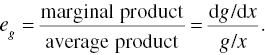
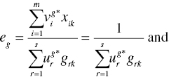
First, let us consider that there is a functional form [![]() ] between a desirable output (g) and an input (x). Then, we measure the degree of desirable output‐based scale elasticity (eg) as follows:
] between a desirable output (g) and an input (x). Then, we measure the degree of desirable output‐based scale elasticity (eg) as follows:
In a similar manner, this chapter considers that cost (c) is expressed by a function of a desirable output (g). The degree of cost‐based scale elasticity (ec) is measured by

Using the two scale elasticity measures, each DMU is classified by the following rule:

On the other hand, the input‐based scale elasticity measures are classified by the following rule:

In the above case, the relationship between the degree of scale elasticity and the type of RTS is same as the cost‐based classification of ec.
Figure 8.1 visually classifies the three types (i.e., increasing, constant, decreasing) of RTS by considering a desirable output‐based model. The figure has two coordinates for x and g. Such a visual description is our convenience. A counter line, connecting {A}–{B}–{C}–{D}, depicts an efficiency frontier. A production possibility set locates within the south‐east region from the efficiency frontier. Paying attention to DMU {B}, for example, Figure 8.1 depicts the three types of slopes and intercepts of a supporting hyperplane.

FIGURE 8.1 Three types of RTS and supporting hyperplanes
Accordingly, Figure 8.1 classifies the three types of desirable output‐based RTS on DMU {B} by the sign of an intercept (σ) as follows:
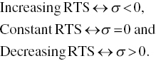

FIGURE 8.2 Type of cost‐based RTS and supporting hyperplane
In a similar manner, Figure 8.2 depicts the three types of RTS that are classified by the cost model. As depicted in the figure, the three types of RTS are characterized by the sign of the intercept (σ) of a supporting hyperplane on a production possibility set that locates within the north‐west region from an efficiency frontier that consists of the four DMUs {A, B, C, D}. The classification becomes opposite to the case of production‐based RTS. The classification is summarized as follows:

Here, it is important to describe four concerns. First, the sign of scale elasticity and the sign of the intercept are based on an input‐oriented RM(v) that is equivalent to the case of the cost model, where RM(v) stands for a radial model under variable RTS. See Chapter 4. Second, RM(c) can assume constant RTS by setting ![]() in the formulation where RM(c) stands for a radial model under the assumption. Third, the scale elasticity is defined by a single desirable output in production economics. DEA can easily extend it to the case of multiple desirable outputs. In the case, the concept, corresponding to “scale elasticity,” is referred to as “scale economies.” Finally, production economics assumes that all DMUs are efficient so that the scale elasticity is measured on an efficiency frontier. In contrast, DEA does not need such an assumption because inefficient DMUs are projected onto the efficiency frontier. Hence, a slack adjustment is necessary for determining the type and magnitude of RTS.
in the formulation where RM(c) stands for a radial model under the assumption. Third, the scale elasticity is defined by a single desirable output in production economics. DEA can easily extend it to the case of multiple desirable outputs. In the case, the concept, corresponding to “scale elasticity,” is referred to as “scale economies.” Finally, production economics assumes that all DMUs are efficient so that the scale elasticity is measured on an efficiency frontier. In contrast, DEA does not need such an assumption because inefficient DMUs are projected onto the efficiency frontier. Hence, a slack adjustment is necessary for determining the type and magnitude of RTS.
A difficulty associated with the proposed DEA‐based RTS measurement is that it contains a possibility in which an infinite number of σ may occur at efficient DMUs such as {A, B, C, D}, all of which consist of vertexes of an efficiency frontier. Such an occurrence is depicted in Figure 8.3. The figure visually describes an occurrence of an infinite number of supporting hyperplanes on DMU {B} and these related intercepts in the case of cost‐based RTS. Therefore, it is necessary for us to examine an upper bound (![]() ) and a lower bound (
) and a lower bound (![]() ) to determine the scale elasticity measures (eg and ec) and to determine the type of RTS by conventional DEA.
) to determine the scale elasticity measures (eg and ec) and to determine the type of RTS by conventional DEA.
FIGURE 8.3 Occurrence of multiple supporting hyperplanes
8.3 PRODUCTION‐BASED RTS MEASUREMENT
As discussed in Section 8.2, the location of a supporting hyperplane determines the type of RTS. Therefore, it is necessary for us to characterize the supporting hyperplane in a data space of multiple inputs and desirable outputs.
As mentioned previously, the RTS measurement is determined by the location of a supporting hyperplane. As a result, we must face an occurrence of multiple supporting hyperplanes, as depicted in Figure 8.3. In the case of RM(v), the upper and lower bounds of the intercept is determined by
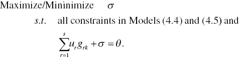
Model (8.18) can be specifically expressed as follows:

Both the primal model (4.4) and the dual model (4.5) are incorporated together in Model (8.18), along with the condition ![]() on optimality. The condition is necessary because the objective value of the primal formulation should equal that of the dual model on optimality. Therefore, the condition needs to be incorporated into Model (8.18).
on optimality. The condition is necessary because the objective value of the primal formulation should equal that of the dual model on optimality. Therefore, the condition needs to be incorporated into Model (8.18).
The upper (![]() ) and lower (
) and lower (![]() ) bounds of σ is identified by maximization or minimization of Model (8.18). It is true that the measurement of upper and lower bounds by Model (8.18) has more constraints than Model (4.5), so being computationally more time‐consuming than Model (4.5). However, the measurement by Model (8.18) is more reliable than that of Model (4.5) in terms of determining the upper (
) bounds of σ is identified by maximization or minimization of Model (8.18). It is true that the measurement of upper and lower bounds by Model (8.18) has more constraints than Model (4.5), so being computationally more time‐consuming than Model (4.5). However, the measurement by Model (8.18) is more reliable than that of Model (4.5) in terms of determining the upper (![]() ) and lower (
) and lower (![]() ) bounds. Thus, there is a tradeoff between them.
) bounds. Thus, there is a tradeoff between them.
To reduce the computational burden, this chapter may approximate Model (8.18) as follows:

Model (8.19) is formulated in the manner that the degree of operational efficiency (OE: ![]() ) on the k‐th DMU, which is determined by Model (4.4), is incorporated in the dual model, or Model (4.5). The upper (under maximization) and lower (under minimization) bounds of σ are obtained after the degree of OE is incorporated into Model (8.19). Thus, Model (8.19) consists of two stages for computation for Model (4.4) and (8.19). Here, IE represents a group of inefficient DMUs that are not on the efficiency frontier. The DMU group (J) stands for all DMUs to be measured by DEA. The group of J‐IE contains DMUs in which clearly inefficient (dominated) DMUs are eliminated from all ones (J). See Chapter 5 for a mathematical definition on J and that of IE.
) on the k‐th DMU, which is determined by Model (4.4), is incorporated in the dual model, or Model (4.5). The upper (under maximization) and lower (under minimization) bounds of σ are obtained after the degree of OE is incorporated into Model (8.19). Thus, Model (8.19) consists of two stages for computation for Model (4.4) and (8.19). Here, IE represents a group of inefficient DMUs that are not on the efficiency frontier. The DMU group (J) stands for all DMUs to be measured by DEA. The group of J‐IE contains DMUs in which clearly inefficient (dominated) DMUs are eliminated from all ones (J). See Chapter 5 for a mathematical definition on J and that of IE.
Model (8.19) has an important feature to be noted here. That is, the dual‐related constraints are also dropped from Model (8.19). It is easily imagined that the computational time to solve Model (8.19) is much less than Model (8.18) because of both less constraints related to inefficient DMUs and no constraints related to the primal and dual formulations. However, the reduced computational effort provides only an approximated range on the intercept, so having a limited classification capability in determining the type of RTS.
After obtaining ![]() and
and ![]() from Model (8.18) or (8.19), the type of input‐based RTS is classified by the following rule:
from Model (8.18) or (8.19), the type of input‐based RTS is classified by the following rule:

As specified in the classification rule (8.20), the input‐oriented RM(v) exhibits increasing RTS on the k‐th DMU if the upper and lower bounds of the intercept are both positive in these signs. In contrast, if they are negative, then the DMU exhibits decreasing RTS. The constant RTS is found on the DMU if the upper bound is positive and the lower bound is negative. The definition on constant RTS is different from production economics because it uses a smooth curve for a production function. In contrast, DEA does not use such a smooth production curve. Such is indeed a strength (i.e., no assumption on a production function) but simultaneously a drawback (i.e. the upper and lower bounds). Thus, DEA is not associated with uniqueness, so suffering from multiple solutions on RTS.
Here, it is necessary to mention that Equations (8.20) is for the input‐based RM(v). The classification becomes opposite in the case when the desirable output‐based RM(v) is employed by DEA. That is,

Note that if we drop the assumption on uniqueness from an intercept (σ) from Equations (8.5), it becomes Equations (8.21). Similarly, the uniqueness changes from Equations (8.6) to Equations (8.21).
8.4 COST‐BASED RTS MEASUREMENT
By shifting our interest from the production‐based RTS measurement to the cost‐based RTS measurement, this chapter starts with Proposition 8.2 which characterizes the location of a supporting hyperplane in a data domain on cost and desirable outputs.
To determine the type of cost‐based RTS, this chapter measures the upper and lower bounds of σ by the following model:

More specifically, Model (8.33) is rewritten by the following formulation:

To reduce our computational burden, this chapter approximates Model (8.33) by the following formulation:

The set (IE) is a group of operationally inefficient DMUs. The minimum cost (![]() ) of the k‐th DMU, measured by Model (4.34), is incorporated in Model (8.34). The model determines the upper (
) of the k‐th DMU, measured by Model (4.34), is incorporated in Model (8.34). The model determines the upper (![]() ) and lower (
) and lower (![]() ) bounds of σ on the estimated cost minimum. As discussed in Section 8.3, Model (8.34) also provides an approximation method to determine the type of RTS.
) bounds of σ on the estimated cost minimum. As discussed in Section 8.3, Model (8.34) also provides an approximation method to determine the type of RTS.
The type of RTS, using the two bounds, is classified by the following rule:

8.5 SCALE EFFICIENCIES AND SCALE ECONOMIES
After returning to the scale economies discussed in Chapter 4, this chapter discusses analytical relationships between production and cost‐based scale efficiencies and scale economies (i.e., RTS).
Proposition 8.3 indicates that a ratio between AEc (allocative and scale efficiency) and AEv (allocative efficiency) indicates the relationship between PSE (production‐based scale efficiency) and CSE (cost‐based scale efficiency). A difficulty in empirical studies is that PSE and CSE can provide qualitative information on scale efficiency measures. However, they cannot provide any quantitative information on scale economies, or a magnitude of RTS.
Hereafter, it is necessary for us to measure the degree of scale economies in multiple components of the two production factors. Here, let eg be the elasticity on production in an input‐oriented model and ec be the elasticity on cost. The two elasticity measures in the case of multiple components are defined as follows:

In the above two equations, the subscripts g and c are added to each dual variable to distinguish between variables obtained from the production model and those from the cost model.
The theoretical relationship between Equations (8.36) and (8.37) is summarized as follows:
As discussed previously, it is possible to drop the assumption on a unique optimal solution on σg *. In the case, let the upper and lower bounds of σg * be ![]() and
and ![]() , then Equation (8.39) can be specified in terms of RTS as follows:
, then Equation (8.39) can be specified in terms of RTS as follows:

In a similar manner, Equation (8.40) is used for the cost‐based RTS as follows:

Applicability:
This chapter does not document an illustrative application of the proposed approach because Chapter 20 will discuss how to measure the type and magnitude of RTS for DEA environmental assessment.
8.6 SUMMARY
This chapter discussed how to measure the type and degree of RTS in a conventional framework of DEA production and cost analyses. The measurement on RTS has often suffered from an occurrence of the three types of multiple solutions. The first one is an occurrence of multiple projections and the second one is an occurrence of multiple reference sets. See Chapter 7, which discusses an occurrence of such multiple solutions. The last one, discussed in this chapter, is an occurrence of multiple intercepts (σ). This chapter considered a range of multiple intercepts by assuming both a unique projection and a unique reference set.
Dual relationships between production‐based RTS and cost‐based RTS were also discussed in this chapter. In Section II, Chapter 20 will extend the concept of RTS into damages to scale (DTS) and Chapter 23 will further extend it to returns to damage (RTD) and damages to return (DTR). Thus, this chapter may serve as conceptual and methodological bases for such a new type of scale economies for DEA environmental assessment.
At the end of this chapter, it is important for us to note that DEA does not assume any functional form to express a production function or a cost function. If we are interested in measuring only a level of efficiency, the unique feature may become a methodological benefit, indeed. However, if we pay attention to the measurement of RTS, the unique feature often becomes a methodological drawback. For example, scale elasticity and scale economies often become very large at the level of infinite. Thus, as discussed in Chapters 22 and 23, DEA environmental assessment needs to restrict multipliers (dual variables) without any prior information. Such a new approach will be discussed as “explorative analysis” in those two chapters.