
24
DISPOSABILITY UNIFICATION
24.1 INTRODUCTION
To measure the level of “corporate sustainability” of organizations in the private sector, this chapter 1 discusses how to unify natural and managerial disposability concepts under radial and non‐radial measurements. See Chapter 15 for a description of corporate sustainability. The proposed approach provides us four unified efficiency measures related to natural disposability and/or managerial disposability. These unified efficiency measures serve as a computational basis for identifying a new type of scale efficiency measures, none of which has been discussed in previous chapters, including Chapter 18.
After theoretically discussing the proposed scale efficiency measures, this chapter applies the proposed approach to examine the level of corporate sustainability among petroleum firms in the United States. The petroleum firms are generally classified into two categories. One of the two categories includes a group of “integrated companies,” which have a large supply chain for spanning both upstream and downstream functions in the US petroleum industry. The other category includes “independent companies” that focus on the upstream function in their business operations.
As an application of the proposed approach, this chapter examines whether the integrated companies outperform the independent companies, because a large supply chain incorporated into the former group provides them with a scale merit in their operations and gives a business opportunity to directly contact consumers2 and identify their opinions on the operation of petroleum firms. Thus, it is easily imagined that a large supply chain can enhance the level of corporate sustainability in the US petroleum industry. Moreover, vertical integration between upstream and downstream may be a promising business trend for better performance in the petroleum industry. This chapter on US industry and Chapter 16 on world industry explore different aspects and structures regarding the petroleum business. See Chapter 13 for a description of the current trend on oil and gas businesses in the world.
The remainder of this chapter is organized as follows. Section 24.2 discusses underlying concepts for disposability unification that are incorporated in the proposed radial and non‐radial approaches. Section 24.3 describes non‐radial measurement under natural, managerial and natural and managerial disposability concepts. Section 24.4 describes radial measurement under the three types of disposability concepts. Section 24.5 discusses a computational flow for disposability unification. Section 24.6 applies the proposed non‐radial and radial approaches to evaluate the unified (environmental and operational) performance of US petroleum companies. Section 24.7 summarizes this chapter.
24.2 UNIFICATION BETWEEN DISPOSABILITY CONCEPTS
Disposability Unification: Returning to Stage III of Figure 15.6, Figure 24.1 visually describes two functional forms in the horizontal axis (x) and in the vertical axis (g and b). One of the two efficiency frontiers, the upper line, expresses the convex relationship between the input (x) and the desirable output (g). The other efficiency frontier indicates a similar (convex) relationship between the input (x) and an undesirable output (b).
FIGURE 24.1 Disposability unification (stage III)
The importance of Figure 15.6 is that it visually describes the three stages (Stages I, II and III) of disposability unification. Figure 24.1 duplicates only the last stage (Stage III) for the unification of natural and managerial disposability concepts. This chapter unifies these disposability concepts based upon Stage III of Figure 15.6.
As identified from the left‐hand side of Figure 24.1, the two efficiency frontiers have an increasing trend of the desirable output (g) and the undesirable output (b) along with an enhanced input (x). The rationale for the shape similarity is because the undesirable output is the “byproduct” of the desirable output. However, as shown on the right‐hand side of Figure 24.1, the two frontiers have different structures. That is, the efficiency frontier for an undesirable output increases and then decreases with input enhancement. As discussed in Chapter 21, such a case occurs under DC, or eco‐technology innovation, for pollution reduction. Thus, the final stage of disposability unification must attain the status of Stage III for the proposed unification, as depicted in both Figure 15.6 and Figure 24.1 because the unification between natural and managerial disposability concepts serves as part of the important process of DEA environmental assessment.
In discussing the proposed disposability unification, it is necessary for us to reorganize Figure 24.1 in the x and g & b space. For this purpose, Figure 24.2 visually specifies the necessary condition for the proposed unification. Figure 24.2 visually assumes that the two types of outputs (g and b) increase with increased input (x). The input change, not listed on the figure, increases the desirable output (g) but decreases the undesirable output (b) from a certain point after eco‐technology is introduced into the operation of an organization. To describe the situation more clearly, Figure 24.2 shows a supporting line that we can identify on the efficiency frontier between g and b. For example, the line (a–c) indicates no occurrence of DC. The line (d–e) shows weak DC that indicates the starting situation on DC. The line (f–h) indicates strong DC, corresponding to the occurrence of eco‐technology innovation on an undesirable output. See Chapter 23 for a detailed description of the three types of DC. In the case of multiple components of the three production factors, the occurrence of strong DC, or the negative slope of the supporting hyperplane, implies that an increase of the input vector leads to an increase in some components of the desirable output vector, but simultaneously decreases some components of an undesirable output vector without worsening the other components. In the disposability unification, it is necessary for us, hereafter, to incorporate such a possible occurrence of strong DC in the proposed formulations.

FIGURE 24.2 Desirable congestion for eco‐technology innovation (a) The three supporting lines (a–c, d–e and f–h) indicate no, weak and strong DC, respectively. The line indicates supporting hyperplanes if it includes an input (x). The figure drops the input for our visual description. (b) It is possible to depict the figure by b on the horizontal axis and g on the vertical axis. In the case, the right‐hand side indicates the occurrence of undesirable congestion (UC). See Chapter 21 for a detailed description on UC. UC is a conventional concept of congestion.
24.3 NON‐RADIAL APPROACH FOR DISPOSABILITY UNIFICATION
UENM under Variable RTS and DTS: Returning to Chapter 16 (non‐radial measurement), this chapter first utilizes a non‐radial model that incorporates the unification of natural and managerial disposability concepts (e.g., Goto et al., 2014). The proposed model is designed to measure the level of unified efficiency under natural and managerial disposability (UENM) of the k‐th DMU.
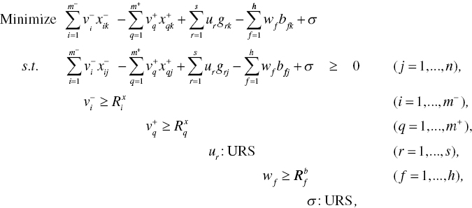
As mentioned in Chapter 16, the k‐th DMU needs to decrease some input(s) and increase some desirable outputs to improve its operational performance under natural disposability. In contrast, the DMU may increase the inputs to improve its environmental performance under managerial disposability. To satisfy the two conflicting requirements, the proposed non‐radial model separates inputs into two categories according to the two disposability concepts. Then, unification of the two disposability concepts uses the following non‐radial (NR) model:

The number of original m inputs are newly separated into ![]() (under natural disposability) and
(under natural disposability) and ![]() (under managerial disposability) in the model in Equation (24.1) in the manner that it maintains m =
(under managerial disposability) in the model in Equation (24.1) in the manner that it maintains m =![]() +
+ ![]() . One of the two input categories uses inputs whose slacks (
. One of the two input categories uses inputs whose slacks (![]() for i = 1,…,
for i = 1,…, ![]() ) are formulated under natural disposability. For example, the number of employees belongs to the input category. The minus in the number of inputs in the first category produces a better performance under natural disposability. The other category contains inputs whose slacks (
) are formulated under natural disposability. For example, the number of employees belongs to the input category. The minus in the number of inputs in the first category produces a better performance under natural disposability. The other category contains inputs whose slacks (![]() for q = 1,…,
for q = 1,…, ![]() ) are formulated under managerial disposability. For example, the amount of capital investment for eco‐technology innovation belongs to the input category. Another example is R&D expenditure. The amount of capital investment is used to attain technology innovation that is important for enhancing the level of production activity and that of environmental protection. The more inputs in the second category produce the better performance under managerial disposability because of green technology development.
) are formulated under managerial disposability. For example, the amount of capital investment for eco‐technology innovation belongs to the input category. Another example is R&D expenditure. The amount of capital investment is used to attain technology innovation that is important for enhancing the level of production activity and that of environmental protection. The more inputs in the second category produce the better performance under managerial disposability because of green technology development.
The level of UENM regarding the k‐th DMU under variable RTS and DTS is determined by

where all slack variables are determined on the optimality of Model (24.1). The equation within the parenthesis, obtained Model (24.1), indicates the level of unified inefficiency under the two disposability concepts. The degree of UENM is obtained by subtracting the level of inefficiency from unity as specified in Equation (24.2).
Model (24.1) has the following dual formulation:

Here, ![]() (i = 1,…,
(i = 1,…, ![]() ),
), ![]() (q = 1,…,
(q = 1,…, ![]() ), ur (r = 1,…, s) and wf (f = 1,…, h) are all dual variables related to the first, second, third and fourth groups of constraints in Model (24.1), respectively. The dual variable (σ), which is unrestricted (URS), is obtained from the last equation of Model (24.1).
), ur (r = 1,…, s) and wf (f = 1,…, h) are all dual variables related to the first, second, third and fourth groups of constraints in Model (24.1), respectively. The dual variable (σ), which is unrestricted (URS), is obtained from the last equation of Model (24.1).
An important feature of Model (24.1) is that it incorporates natural and managerial disposability in such a manner that inputs and two types of outputs are classified by the two disposability concepts. In the previous chapters, these disposability concepts are equally treated in the evaluation of UENM.
Problem of Model (24.3): The supporting hyperplane, obtained by Model (24.3), becomes ![]() in a simple case where three production factors have a single component. The simple case is for our descriptive convenience. This chapter considers that
in a simple case where three production factors have a single component. The simple case is for our descriptive convenience. This chapter considers that ![]() stands for an amount for eco‐technology investment, for example. The supporting hyperplane indicates
stands for an amount for eco‐technology investment, for example. The supporting hyperplane indicates ![]() where all the dual variables, except σ, are positive. The dual variable (σ) is unrestricted in sign. It is easily thought that the supporting hyperplane does not fit with our expectation. For instance, an increase in the input (
where all the dual variables, except σ, are positive. The dual variable (σ) is unrestricted in sign. It is easily thought that the supporting hyperplane does not fit with our expectation. For instance, an increase in the input (![]() ) decreases the undesirable output because of
) decreases the undesirable output because of ![]() . The sign should be opposite. The following three conditions are necessary for us to make the supporting hyperplane fit with our expectation to apply DEA to performance analysis for energy and environment. First, if
. The sign should be opposite. The following three conditions are necessary for us to make the supporting hyperplane fit with our expectation to apply DEA to performance analysis for energy and environment. First, if ![]() increases or decreases, then b increases or decreases because
increases or decreases, then b increases or decreases because ![]() is the input under natural disposability. Second, if
is the input under natural disposability. Second, if ![]() increases or decreases, then b decreases or increases because
increases or decreases, then b decreases or increases because ![]() indicates the input under managerial disposability (e.g., eco‐technology investment). Thus, the two expectations clearly indicate that the unknown parameter (
indicates the input under managerial disposability (e.g., eco‐technology investment). Thus, the two expectations clearly indicate that the unknown parameter (![]() ) should be positive and the other (
) should be positive and the other (![]() ) should be negative in their signs, respectively. Finally, both u and σ should be unrestricted in these signs to incorporate the possible occurrence of DC, as depicted in Figure 24.2, where the slope of the supporting hyperplane is determined by u and the intercept is determined by σ. Consequently, the supporting hyperplane should be
) should be negative in their signs, respectively. Finally, both u and σ should be unrestricted in these signs to incorporate the possible occurrence of DC, as depicted in Figure 24.2, where the slope of the supporting hyperplane is determined by u and the intercept is determined by σ. Consequently, the supporting hyperplane should be ![]() in the simple case.
in the simple case.
UENM(DC): To reorganize Model (24.3) in such a manner that it can fit with Figure 24.2, Sueyoshi and Goto (2014b) proposed the following non‐radial model in which the k‐th DMU can simultaneously attain the status of natural and managerial disposability along with the possible occurrence of desirable congestion (DC):
where vi (i = 1,…, ![]() ), vq (q = 1,…,
), vq (q = 1,…, ![]() ), ur (r = 1,…, s) and wf (f = 1,…, h) are parameters to express the direction of the supporting hyperplane measured by Model (24.4). The dual variable (σ), which is unrestricted (URS), indicates the intercept of the expected supporting hyperplane.
), ur (r = 1,…, s) and wf (f = 1,…, h) are parameters to express the direction of the supporting hyperplane measured by Model (24.4). The dual variable (σ), which is unrestricted (URS), indicates the intercept of the expected supporting hyperplane.
Model (24.4), which is a dual model, has the following primal (dual’s dual) formulation that unifies the two disposability concepts:
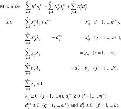
Model (24.5) has two unique features in the structure. One of the two features is that all the inputs are classified into two categories, as mentioned previously. The first category includes a group of inputs whose slacks (![]() for i = 1,…,
for i = 1,…, ![]() ) are formulated under natural disposability. The other category contains a group of inputs whose slacks (
) are formulated under natural disposability. The other category contains a group of inputs whose slacks (![]() for q = 1,…,
for q = 1,…, ![]() ) are formulated under managerial disposability. The other unique feature is that the constraints regarding a desirable output vector
) are formulated under managerial disposability. The other unique feature is that the constraints regarding a desirable output vector ![]() are expressed by equality because they do not have any slacks. In contrast, the other groups of constraints are expressed by inequality because they have slacks in Model (24.5). The existence of slacks indicates the status of inequality.
are expressed by equality because they do not have any slacks. In contrast, the other groups of constraints are expressed by inequality because they have slacks in Model (24.5). The existence of slacks indicates the status of inequality.
The unified efficiency under natural and managerial disposability, or ![]() , of the k‐th DMU is measured by
, of the k‐th DMU is measured by

where all slack variables are determined on the optimality of Model (24.5). The equation within the parenthesis, obtained from the optimality of Model (24.5), indicates the level of unified inefficiency under natural and managerial disposability. The level of unified efficiency is obtained by subtracting the level of inefficiency from unity under the occurrence of DC, or eco‐technology innovation, on undesirable outputs. It is important to note that Models (24.4) and (24.5) under non‐radial measurement, corresponding to Stage III of Figure 15.6.
UENM(DC) under Constant RTS and DTS: Model (24.5) may drop ![]() from the formulation as follows:
from the formulation as follows:
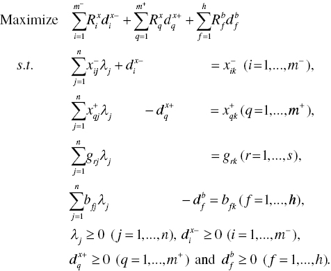
Model (24.7) drops ![]() from the formulation. Then, Equation (24.6) measures the level of
from the formulation. Then, Equation (24.6) measures the level of ![]() under constant RTS and DTS as follows:
under constant RTS and DTS as follows:
where all slacks are determined on the optimality of Model (24.7). The subscript c stands for constant RTS and DTS, so not the subscript v in Equation (24.8).
Scale Efficiency under Natural and Managerial Disposability: After obtaining the two types of UENM(DC) for the k‐th DMU, this chapter uses
to determine the level of scale efficiency in the case of non‐radial models. The scale efficiency indicates the level at which each DMU effectively operates by considering the operational size. Thus, the degree of scale efficiency can be considered as a level of efficiency for size utilization under the possible occurrence of eco‐technology innovation.
At the end of this section, it is important to note that the magnitude control factor (MCF: ε) is usually incorporated into the proposed non‐radial models. See Chapter 16 which discusses the use of MCF in the non‐radial approach. Since Chapter 16 has not used the MCF in its empirical study on petroleum firms, this chapter does not incorporate it in the proposed formulations, in order to maintain empirical consistency between Chapter 16 and this chapter.
24.4 RADIAL APPROACH FOR DISPOSABILITY UNIFICATION
UENM under variable RTS and DTS: Since Chapter 17 has already discussed Stage I of Figure 15.6, this chapter starts with Stage II for radial measurement. First, shifting our description from a non‐radial (Section 24.3) to a radial approach, this chapter follows the previous research of Sueyoshi and Goto (e.g., Sueyoshi and Goto 2012b, 2014a) that proposed the following radial (R) model that corresponds to Model (24.1):

Model (24.10) combines Models (17.5) and (17.10) by a straightforward unification. The level of ![]() regarding the k‐th DMU under variable RTS and DTS is determined by
regarding the k‐th DMU under variable RTS and DTS is determined by

where all slacks are determined on the optimality of Model (24.10). The equation within the parentheses, obtained from the optimality of Model (24.10), indicates the level of unified inefficiency. The UENM is obtained by subtracting the level of inefficiency from unity.
The dual formulation of Model (24.10) becomes as follows:

As discussed for UENM measured by the non‐radial approach, Models (24.10) and (24.12) have a difficulty in measuring technology innovation, as well. A description on the rationale in Section 24.3 is applicable to Models (24.10) and (24.12).
UENM(DC): To discuss the structure of the supporting hyperplane, as depicted in Figure 24.2, this chapter reorganizes Model (24.12) whose hyperplane becomes ![]() in the case where three production factors have a single component. The corresponding formulation of Model (24.12), satisfying the requirement on the case of multiple components, becomes as follows:
in the case where three production factors have a single component. The corresponding formulation of Model (24.12), satisfying the requirement on the case of multiple components, becomes as follows:

Along with the slight modification, Model (24.13) drops ![]() from the second constraint of Model (24.12). The rationale is that
from the second constraint of Model (24.12). The rationale is that ![]() may be infeasible because ur is unrestricted in the sign so that the dual variable cannot become negative, or the equation becomes infeasible in the worst case. To avoid such a computational difficulty, this chapter reorganizes Model (24.12) with a structure like Model (24.13).
may be infeasible because ur is unrestricted in the sign so that the dual variable cannot become negative, or the equation becomes infeasible in the worst case. To avoid such a computational difficulty, this chapter reorganizes Model (24.12) with a structure like Model (24.13).
The primal (dual’s dual) formulation of Model (24.13) becomes as follows:

Model (24.14) corresponds to Model (24.5) in the non‐radial measurement. The level of ![]() regarding the k‐th DMU under variable RTS and DTS is determined by
regarding the k‐th DMU under variable RTS and DTS is determined by

where the inefficiency score and all slack variables are determined by the optimality of Model (24.14). The equation within the parentheses, obtained from Model (24.14), indicates the level of unified inefficiency. The degree of ![]() is obtained by subtracting the level of inefficiency from unity. Here, the magnitude of the inefficiency score (ξ*) is determined by desirable outputs in Model (24.14) because these outputs are byproducts of desirable outputs. The influence of undesirable outputs exists as slacks on undesirable outputs
is obtained by subtracting the level of inefficiency from unity. Here, the magnitude of the inefficiency score (ξ*) is determined by desirable outputs in Model (24.14) because these outputs are byproducts of desirable outputs. The influence of undesirable outputs exists as slacks on undesirable outputs ![]() , as specified in Equation (24.15). It is important to note that Models (24.13) and (24.14) under radial measurement correspond to Stage III of Figure 15.6.
, as specified in Equation (24.15). It is important to note that Models (24.13) and (24.14) under radial measurement correspond to Stage III of Figure 15.6.
Meanwhile, under constant RTS and DTS, the level of ![]() regarding the k‐th DMU is determined by
regarding the k‐th DMU is determined by

The degree of ![]() on the k‐th DMU under constant RTS and DTS is determined by
on the k‐th DMU under constant RTS and DTS is determined by
All the slack variables used in Equation (24.17) are determined by the optimality of Model (24.16).
Scale Efficiency under Natural and Managerial Disposability: After obtaining the two types of UENM(DC), this chapter measures
as the level of scale efficiency in the case of radial measurement.
24.5 COMPUTATIONAL FLOW FOR DISPOSABILITY UNIFICATION
Figure 24.3 visually describes the computational flow for disposability unification and efficiency measurement. Although this chapter uses non‐radial models for our empirical study, this description can be applied to the radial framework.

FIGURE 24.3UENM(DC) and efficiency measures (a) It is possible for us to apply the proposed approach to both radial and non‐radial measurements. Therefore, this chapter does not specify R (radial) and NR (non‐radial) in the figure.
As depicted in Figure 24.3, the proposed approach measures the level of unified efficiency (UE). See Chapters 16 and 17 on UE measurement. As discussed in the two chapters, we measure UE under natural disposability (UEN) and UE under managerial disposability (UEM). After measuring UE, UEN and UEM, the proposed approach combines two disposability concepts for a unified efficiency measure (UENM). By unifying them, this chapter considers two conditions related to the occurrence of congestion. One of the two conditions is that it is possible for us to measure UENM under no occurrence of undesirable congestion (UC). The other condition is that we can consider the possible occurrence of desirable congestion (DC), or eco‐technology innovation on undesirable outputs, to measure the level of UENM(DC). The rationale on the first condition is that this chapter is interested in measuring the level of scale efficiency (SENM) on US petroleum companies. In this case, it is necessary for us to assume that no UC occurs in the transportation system from upstream to downstream. As a result, this chapter can determine the degree of SENM(DC). Meanwhile, the rationale on the second condition is because this chapter is interested in the performance assessment of US petroleum companies under a possible occurrence of eco‐technology innovation and its related managerial challenge.
Figure 24.4 visually describes the computation of SENM(DC) in the horizontal axis (x: input) and the vertical axis (g: desirable output; b: undesirable output). The efficiency frontier for the desirable output is a piece‐wise linear contour line ({A}–{B}–{C}–{D}–{E}) and that of the undesirable output is the contour line ({F}–{G}–{H}–{I}–{J}–{K}). The upper contour line has an increasing shape because it is structured by no occurrence of UC, while the other (lower) one has an increasing and decreasing shape because it is structured by the possible occurrence of DC, or eco‐technology innovation. Based upon the type of RTS and DTS, this chapter classifies the efficiency frontier for the desirable output into two cases. One of the two cases is the contour line ({A}–{B}–{C}–{D}–{E}) under variable RTS. The other case is the straight line from the origin (O) to L that is structured by constant RTS.

FIGURE 24.4SENM(DC) measurement (a) RTS: returns to scale; DTS: damages to scale; DC: desirable congestion. (b) DMU {P} is projected onto N on the contour line segments {A}–{B}–{C}–{D}–{E} (the efficiency frontier for the desirable output under variable RTS). Meanwhile, it is projected onto L on the line from the origin O to L. The level of efficiency is determined by the distance between the observed point and the projected point. After disposability unification, the distance is measured by the desirable output. (c) The line segments, or {F}–{G}–{H}–{I}–{J}–{K}, consist of the efficiency frontier for the undesirable output. The frontier is shaped by variable DTS and the possible occurrence of desirable congestion (DC), or eco‐technology innovation. (d) This figure incorporates the possible occurrence of DC, but excludes UC. As a result, the frontier for desirable output has an increasing shape and the frontier for undesirable output has an increasing and decreasing shape. This figure incorporates the assumption that the undesirable output is a byproduct of the desirable output. Without this assumption, the efficiency frontier has a concave shape, not a convex shape as depicted in this figure. See Figure 15.6.
Assuming that the undesirable output is a byproduct of the desirable output, this chapter measures the magnitude of UENM(DC)v on the observed DMU{P} by dividing the distance between {P} and Q by the distance between N and Q under variable RTS. Meanwhile, the magnitude of UENM(DC)c is measured by the distance between {P} and Q divided by that between L and Q under constant RTS. Consequently, the degree of SENM(DC) is measured by

The degree indicates the ratio between distance N to Q divided by that between L to Q. The assumption on “byproduct” makes it possible to measure the degree of SENM(DC) based upon the magnitude of desirable outputs. See Models (24.14) and (24.16).
24.6 US PETROLEUM INDUSTRY
24.6.1 Data
This chapter utilizes a data set on US oil and natural gas production companies, all of which are listed in the New York Stock Exchange (NYSE) Energy Index (2013)3. The index covers 82 independent producers and 20 integrated companies. This chapter restricts the proposed approach to petroleum companies4 whose operations are in the United States. The amount of their greenhouse gas (GHG) emissions is obtained from the EPA’s GHG Reporting Program (2013)5. This program required facilities emitting more than 25,000 metric tons of CO2 equivalents per year to submit reports on GHG emissions from 2010. The sources covered by the program account for 85–90% of the total GHG emission in the United States. The emission data set is reported at the facility level. Each company may operate multiple oil and gas projects in different regions. This chapter extracts the emission data from all onshore oil/gas production sites and then aggregates them at corporate level.
Data Accessibility: The supplementary section of Sueyoshi and Wang (2014b) contains the whole data set used in this study.
Each company’s emission is closely related to its drilling activity. Therefore, this chapter extracts the number of wells drilled by a company from the annual report. In alignment with the emission data, the drilled wells used in this chapter count only those drilled onshore in the United States. We also obtain the three‐year average for 2010–2012 on acquisition, finding and development (AFD) expenses from Ernst Young (2013)6. The AFD expenses reflect each companies’ abilities to access and obtain petroleum reserves, which indirectly affect their GHG emission. A higher acquisition cost is generally paid for easy accessibility to resources which require less effort to drill, hence incurring a lower emission. A higher finding and development cost may imply more intensive exploration, hence producing more emissions from exploration. Finally, this chapter collects the companies’ financial and operational data from the COMPUSTAT database. The data set used in this chapter is summarized below in detail.
- GHG Emission: This measures the amount of emissions from each firm’s onshore production, including not only CO2 but also methane (CH4) and nitrous oxide (N2O). The cost of adapting pollution prevention practices and the effectiveness of pollution prevention as a strategy for reducing emissions may vary with the scale of current emission.
- Number of Employees: This is regarded as a proxy for corporate size. Larger firms may have more resources to adapt GHG mitigation practices.
- Capital Expenditure: This is included to indicate the operating liquidity of a firm. Firms with higher capital expenditure may invest more in GHG mitigation.
- R&D Expense: This is a measure of a firm’s technology capacity and serves as a proxy for technology innovation. It is expected that firms with higher R&D expense is more likely to acquire and implement efficient emission control technology.
- Total Assets: This includes current assets, property, plant and equipment, all of which are used as another proxy for corporate size.
- Net Number of Wells Drilled: This gives the number of wells drilled by a company for the calendar year, accounting for the fractional working interest owned by the company in each well. For instance, a 50% interest in a well is counted as 0.5 well.
- Revenue: This is income received from the sale of oil and gas and indicates the operational size of the business.
- Acquisition, Finding and Development (AFD) Expense: This is calculated as the sum of proved reserve acquisition cost and the finding and development cost. Specifically, the proved reserve acquisition cost is calculated as the reserve purchasing cost divided by the reserve purchased. The finding and development cost is calculated as the unproved reserve acquisition cost, exploration and development expenditures relative to the added reserve. Overall, this chapter computes the sum of AFD costs as the aggregate measure of each company’s ability to obtain access to per barrel of oil equivalent (BOE) resources.
This chapter utilizes the amount of total revenue as a desirable output and the amount of GHG emission as an undesirable output. The five inputs under natural disposability include the number of employees, an amount of capital expenditure, a total amount of assets, the number of net wells drilled, and an amount of total AFD expense. The other input under managerial disposability is an amount of R&D expenditure.
In collecting the data set, this chapter removed companies with data missing from any of the relevant fields. Eventually, this chapter obtained a set of 50 companies (n = 50), including 43 independent companies and seven integrated companies. The data set consists of roughly half of all production companies in the NYSE Energy Index. Meanwhile, the total emission from these 50 companies is 82.3 MMT7 emissions from the entire onshore production segment in the United States. Here, MMT stands for methylcyclopentadienyl manganese tricarbonyl.
The descriptive statistics of the data set used for this chapter are listed in Sueyoshi and Wang (2014b). According their study, integrated companies are larger than independent companies in all data fields, on average. The GHG emissions by integrated firms have an average of 6849.6230 thousand tons, being 8.8 times the average emission of 775.4225 thousand tons produced by independent companies. The largest emission of 24,529 thousand tons comes from Exxon Mobil, whereas EnCana Corporation has the smallest emission of 110 thousand tons. The integrated companies drill 468 wells on average, 36% more than the independent companies. However, the most active driller, Occidental Petroleum Corporation (1411.2 net wells drilled) is an independent company.
24.6.2 Unified Efficiency Measures
Table 24.1 documents the five efficiency measures, along with the p‐value of the t‐test at the bottom, to confirm whether integrated oil companies outperform independent ones. These unified efficiency scores are measured by the non‐radial approach. For example, UE, UEN, UEM, UENM and UENM(DC) are solved by Models (16.1), (16.6), (16.12), (24.1) and (24.5), respectively. Thus, they correspond to ![]() ,
, ![]() ,
, ![]() ,
, ![]() and
and ![]() , respectively. As mentioned previously, this chapter uses only the non‐radial measurement, not the radial measurement, to maintain consistency with the research effort of Chapter 16 that compared national and international companies.
, respectively. As mentioned previously, this chapter uses only the non‐radial measurement, not the radial measurement, to maintain consistency with the research effort of Chapter 16 that compared national and international companies.
TABLE 24.1 Unified efficiency measures: non‐radial approach
(a) Source: Sueyoshi and Wang (2014b). (b) Avg., Max., Min. and S.D. stand for average, minimum, maximum, and standard deviation, respectively.
| Company Name | UE | UEN | UEM | UENM | UENM(DC) |
| Independent companies | |||||
| Anadarko Petroleum Corporation | 1.0000 | 0.7495 | 1.0000 | 1.0000 | 1.0000 |
| Antero Resources LLC | 1.0000 | 1.0000 | 0.7837 | 1.0000 | 1.0000 |
| Apache Corporation | 1.0000 | 0.7484 | 0.8878 | 0.9390 | 1.0000 |
| Berry Petroleum Company | 1.0000 | 1.0000 | 0.6758 | 0.9312 | 1.0000 |
| BHP Billiton Group | 1.0000 | 1.0000 | 1.0000 | 1.0000 | 1.0000 |
| Bill Barrett Corporation | 0.9999 | 0.9627 | 0.7163 | 0.9591 | 0.9904 |
| Cabot Oil & Gas Corporation | 1.0000 | 1.0000 | 0.6473 | 1.0000 | 1.0000 |
| Chesapeake Energy Corporation | 1.0000 | 0.7335 | 0.8467 | 0.8112 | 1.0000 |
| Cimarex Energy Co. | 0.9584 | 0.9683 | 0.7488 | 0.9713 | 0.9773 |
| Concho Resources | 1.0000 | 0.9156 | 0.8873 | 0.9196 | 0.9218 |
| Conoco Phillips | 1.0000 | 0.7910 | 0.7811 | 1.0000 | 1.0000 |
| CONSOL Energy Inc. | 0.9991 | 1.0000 | 0.8400 | 0.9760 | 0.9766 |
| Continental Resources, Inc. | 1.0000 | 0.9438 | 0.7977 | 0.9457 | 0.9495 |
| Denbury Resources Inc. | 0.9998 | 1.0000 | 0.8991 | 0.9758 | 0.9758 |
| Devon Energy Corporation | 1.0000 | 0.8070 | 0.6644 | 0.9479 | 1.0000 |
| EnCana Corporation | 1.0000 | 1.0000 | 1.0000 | 1.0000 | 1.0000 |
| Energen Corporation | 0.9999 | 0.9467 | 0.8391 | 0.9474 | 0.9503 |
| EOG Resources, Inc. | 1.0000 | 0.8622 | 0.7984 | 0.8836 | 0.8899 |
| EP Energy LLC | 1.0000 | 0.9725 | 0.7805 | 1.0000 | 1.0000 |
| EQT Corporation | 0.9967 | 0.9639 | 0.8401 | 0.9760 | 0.9781 |
| EXCO Resources, Inc. | 1.0000 | 0.9723 | 0.8253 | 0.9724 | 0.9999 |
| Forest Oil Corporation | 0.9277 | 0.9134 | 0.8418 | 0.9136 | 0.9281 |
| Laredo Petroleum Holdings, Inc. | 0.9997 | 1.0000 | 0.8886 | 1.0000 | 1.0000 |
| Linn Energy, LLC | 1.0000 | 1.0000 | 0.7266 | 0.9363 | 0.9444 |
| National Fuel Gas Company | 0.9824 | 0.9088 | 1.0000 | 0.9008 | 0.9015 |
| Newfield Exploration Company | 0.9552 | 0.9266 | 0.8115 | 0.9300 | 0.9350 |
| Noble Energy, Inc. | 1.0000 | 0.8978 | 0.7896 | 0.9520 | 1.0000 |
| Occidental Petroleum Corporation | 1.0000 | 0.6949 | 1.0000 | 0.8167 | 0.8192 |
| PDC Energy, Inc. | 1.0000 | 0.9878 | 0.7750 | 1.0000 | 1.0000 |
| Pioneer Natural Resources Company | 1.0000 | 0.8931 | 0.7334 | 0.9244 | 0.9398 |
| Plains E & P Company | 1.0000 | 1.0000 | 1.0000 | 1.0000 | 0.9142 |
| QEP Resources, Inc. | 0.9809 | 0.9410 | 0.7821 | 0.9410 | 0.9462 |
| Quicksilver Resources, Inc. | 0.9998 | 1.0000 | 0.8719 | 1.0000 | 1.0000 |
| Range Resources Corporation | 0.9999 | 0.9464 | 0.9061 | 1.0000 | 1.0000 |
| Rosetta Resources Inc. | 1.0000 | 1.0000 | 0.8031 | 1.0000 | 1.0000 |
| SandRidge Energy, Inc. | 1.0000 | 0.8932 | 0.6766 | 0.8917 | 1.0000 |
| SM Energy Company | 1.0000 | 0.9551 | 0.6941 | 0.9619 | 1.0000 |
| Southwestern Energy Company | 1.0000 | 1.0000 | 0.9359 | 1.0000 | 1.0000 |
| Swift Energy Inc. | 0.9998 | 0.9750 | 0.9152 | 0.9785 | 1.0000 |
| Talisman Energy Inc. | 0.9767 | 0.9146 | 0.8075 | 0.9230 | 0.9269 |
| Ultra Petroleum Corporation | 1.0000 | 1.0000 | 1.0000 | 1.0000 | 1.0000 |
| Whiting Petroleum Corporation | 0.9485 | 0.9295 | 0.8398 | 1.0000 | 1.0000 |
| WPX Energy, Inc. | 0.9797 | 0.9311 | 0.7222 | 0.9402 | 0.9488 |
| Avg. | 0.9931 | 0.9313 | 0.8321 | 0.9574 | 0.9724 |
| Max. | 1.0000 | 1.0000 | 1.0000 | 1.0000 | 1.0000 |
| Min. | 0.9277 | 0.6949 | 0.6473 | 0.8112 | 0.8192 |
| S.D. | 0.0163 | 0.0825 | 0.1022 | 0.0473 | 0.0407 |
| Integrated companies | |||||
| BP PLC | 1.0000 | 1.0000 | 1.0000 | 1.0000 | 1.0000 |
| Chevron Corporation | 1.0000 | 1.0000 | 1.0000 | 1.0000 | 1.0000 |
| Exxon Mobil Corporation | 1.0000 | 1.0000 | 1.0000 | 1.0000 | 1.0000 |
| Hess Corporation | 1.0000 | 0.8498 | 0.7055 | 1.0000 | 1.0000 |
| Marathon Oil Corporation | 1.0000 | 1.0000 | 0.6733 | 1.0000 | 1.0000 |
| Murphy Oil Corporation | 1.0000 | 1.0000 | 0.8192 | 1.0000 | 1.0000 |
| Royal Dutch Shell PLC | 1.0000 | 1.0000 | 1.0000 | 1.0000 | 1.0000 |
| Avg. | 1.0000 | 0.9785 | 0.8854 | 1.0000 | 1.0000 |
| Max. | 1.0000 | 1.0000 | 1.0000 | 1.0000 | 1.0000 |
| Min. | 1.0000 | 0.8498 | 0.6733 | 1.0000 | 1.0000 |
| S.D. | 0.0000 | 0.0568 | 0.1496 | 0.0000 | 0.0000 |
| P‐value (Welch’s t‐test) | 0.0085 | 0.0849 | 0.3937 | 0.0000 | 0.0001 |
In Table 24.1, the worst performers among the independent companies are Forest Oil in UE, Occidental Petroleum in UEN, Cabot Oil and Gas Corporation in UEM, Chesapeake Energy Corporation in UENM and Occidental Petroleum in UENM(DC) on average efficiency. Among the integrated companies, the worst performers are Hess Corporation in UEN and Marathon Oil in UEM. All seven integrated companies have an efficiency of 1.0000 in UE, UENM and UENM(DC). Moreover, there are seven companies with an efficiency score of 1.0000 in all five measures, including three independent companies (i.e., Billiton, EnCana and Ultra Petroleum) and four integrated companies (i.e., BP, Chevron, Exxon Mobil and Royal Dutch Shell). On average, Occidental Petroleum and Chesapeake Energy have the lowest efficiency scores. The relatively low performance of both companies can be partly attributed to their significant stake in shale productions.
The development of shale wells releases more GHG, especially methane, than conventional wells due to hydraulic fracturing8. The EPA has issued new rules to reduce air emissions from hydraulic fracturing9. In addition, the low price of natural gas in recent years has also undermined their revenues.
Overall, the efficiency score of the independent petroleum companies are 0.9931 in UE, 0.9313 in UEN, 0.8321 in UEM, 0.9574 in UENM and 0.9724 in UENM(DC), on average, while the respective scores, on average, of the integrated companies are 1.0000, 0.9785, 0.8854, 1.0000 and 1.0000. Thus, on average, the integrated companies outperform the independent companies in terms of all five efficiency measures. The largest difference occurs in UEM and the smallest difference occurs in UE.
This chapter applied the t‐test to the efficiency scores of the integrated and independent companies. The results in the bottom row of the table indicate that the integrated companies have higher UE, UENM and UENM(DC) than the independent companies at the 1% significance level, and higher UEN at the 10% significance level. Therefore, we consider that firms with a supply chain outperform those without a supply chain. An exception can be found in the t‐test on UEM between the two groups because US environmental regulation is equally effective on the two types of petroleum firms.
The results in Table 24.1 also imply that the unified (operational and environmental) performance of US petroleum firms is positively affected by the size of their supply chains. In fact, the four most consistently efficient integrated companies have more branded retail outlets than the other integrated companies10. A larger retail network is associated with a higher visibility to consumers, hence resulting in higher market pressure on the unified performance. It can be conjectured that consumer pressure in the downstream spreads over the supply chain and has an impact on the performance of exploration and production in the upstream.
24.6.3 Scale Efficiency
As mentioned previously, the petroleum industry can be considered as a very large process industry from the exploration of oil and gas to the retail services for end users. Chakravarthy (1997)11 and Vachon and Klassen (2006)12 have discussed that petroleum firms may have increasing difficulties in planning and predicting their businesses when their corporate size grows. Thus, it is necessary for us to examine how they manage a unified performance from the perspective of their business size. In other words, it is expected that, since the integrated companies are much larger than the independent companies, their business operations are more difficult than that of the independent companies.
To investigate the magnitude of scale efficiency, this chapter measures a degree of UENM(DC) under the possible occurrence of DC. The degree of ![]() under variable RTS is measured by Model (24.5). The degree of
under variable RTS is measured by Model (24.5). The degree of ![]() under constant RTS is measured by Model (24.7) after dropping
under constant RTS is measured by Model (24.7) after dropping ![]() into the formulation. One important feature of these two efficiency measures is that both incorporate the possible occurrence of DC, or eco‐technology innovation, but exclude the occurrence of UC. The difference can be found in the type of RTS in their formulations.
into the formulation. One important feature of these two efficiency measures is that both incorporate the possible occurrence of DC, or eco‐technology innovation, but exclude the occurrence of UC. The difference can be found in the type of RTS in their formulations.
After obtaining the two measures for each DMU, this chapter measures the degree of scale efficiency: SENM(DC) by Equation (24.9). The scale efficiency measures how each DMU effectively operates by considering the operational size. Thus, the magnitude of SENM(DC) indicates the level of efficiency in the effective size utilization of each DMU operation.
Table 24.2 summarizes UENM(DC)v, UENM(DC)c and SENM(DC) regarding all independent and integrated petroleum companies. Here, the three unified efficiencies are measured by Models (24.5) and (24.7) along with Equation (24.9), respectively. The SENM of independent firms is 0.9864 and that of integrated companies is 1.0000 on average. The t‐test confirms at the 1% significance that the integrated companies outperform the independent companies in terms of their size utilization. This result implies that the integrated companies may have more managerial difficulty, along with an increase in their operational size, than the independent companies. However, by carefully controlling their large supply chains from exploration to retail services, the integrated companies can effectively increase their unified (operational and environmental) performance, so being able to enhance the level of corporate sustainability.
TABLE 24.2 Scale efficiency measures: non‐radial approach
(a) Source: Sueyoshi and Wang (2014b).
| Company Name | UENM(DC)v | UENM(DC)c | Scale Efficiency (DC) |
| Independent companies | |||
| Anadarko Petroleum Corporation | 1.0000 | 1.0000 | 1.0000 |
| Antero Resources LLC | 1.0000 | 1.0000 | 1.0000 |
| Apache Corporation | 1.0000 | 1.0000 | 1.0000 |
| Berry Petroleum Company | 1.0000 | 1.0000 | 1.0000 |
| BHP Billiton Group | 1.0000 | 1.0000 | 1.0000 |
| Bill Barrett Corporation | 0.9904 | 0.9875 | 0.9970 |
| Cabot Oil & Gas Corporation | 1.0000 | 1.0000 | 1.0000 |
| Chesapeake Energy Corporation | 1.0000 | 0.8884 | 0.8884 |
| Cimarex Energy Co. | 0.9773 | 0.9693 | 0.9917 |
| Concho Resources | 0.9218 | 0.9094 | 0.9865 |
| Conoco Phillips | 1.0000 | 1.0000 | 1.0000 |
| CONSOL Energy Inc. | 0.9766 | 0.9601 | 0.9830 |
| Continental Resources, Inc. | 0.9495 | 0.9395 | 0.9894 |
| Denbury Resources Inc. | 0.9758 | 0.9576 | 0.9814 |
| Devon Energy Corporation | 1.0000 | 1.0000 | 1.0000 |
| EnCana Corporation | 1.0000 | 1.0000 | 1.0000 |
| Energen Corporation | 0.9503 | 0.9410 | 0.9902 |
| EOG Resources, Inc. | 0.8899 | 0.8817 | 0.9907 |
| EP Energy LLC | 1.0000 | 1.0000 | 1.0000 |
| EQT Corporation | 0.9781 | 0.9665 | 0.9881 |
| EXCO Resources, Inc. | 0.9999 | 0.9693 | 0.9694 |
| Forest Oil Corporation | 0.9281 | 0.9279 | 0.9999 |
| Laredo Petroleum Holdings, Inc. | 1.0000 | 0.9666 | 0.9666 |
| Linn Energy, LLC | 0.9444 | 0.9404 | 0.9958 |
| National Fuel Gas Company | 0.9015 | 0.8868 | 0.9836 |
| Newfield Exploration Company | 0.9350 | 0.9276 | 0.9921 |
| Noble Energy, Inc. | 1.0000 | 1.0000 | 1.0000 |
| Occidental Petroleum Corporation | 0.8192 | 0.8102 | 0.9890 |
| PDC Energy, Inc. | 1.0000 | 1.0000 | 1.0000 |
| Pioneer Natural Resources Company | 0.9398 | 0.9386 | 0.9988 |
| Plains E & P Company | 0.9142 | 0.8965 | 0.9806 |
| QEP Resources, Inc. | 0.9462 | 0.9378 | 0.9912 |
| Quicksilver Resources, Inc. | 1.0000 | 0.9847 | 0.9847 |
| Range Resources Corporation | 1.0000 | 1.0000 | 1.0000 |
| Rosetta Resources Inc. | 1.0000 | 1.0000 | 1.0000 |
| SandRidge Energy, Inc. | 1.0000 | 0.9168 | 0.9168 |
| SM Energy Company | 1.0000 | 0.9899 | 0.9899 |
| Southwestern Energy Company | 1.0000 | 0.9462 | 0.9462 |
| Swift Energy Inc. | 1.0000 | 0.9387 | 0.9387 |
| Talisman Energy Inc. | 0.9269 | 0.9154 | 0.9876 |
| Independent companies | |||
| Ultra Petroleum Corporation | 1.0000 | 1.0000 | 1.0000 |
| Whiting Petroleum Corporation | 1.0000 | 1.0000 | 1.0000 |
| WPX Energy, Inc. | 0.9488 | 0.9457 | 0.9967 |
| Avg. | 0.9724 | 0.9591 | 0.9864 |
| Max. | 1.0000 | 1.0000 | 1.0000 |
| Min. | 0.8192 | 0.8102 | 0.8884 |
| S.D. | 0.0407 | 0.0444 | 0.0233 |
| Integrated companies | |||
| BP PLC | 1.0000 | 1.0000 | 1.0000 |
| Chevron Corporation | 1.0000 | 1.0000 | 1.0000 |
| Exxon Mobil Corporation | 1.0000 | 1.0000 | 1.0000 |
| Hess Corporation | 1.0000 | 1.0000 | 1.0000 |
| Marathon Oil Corporation | 1.0000 | 1.0000 | 1.0000 |
| Murphy Oil Corporation | 1.0000 | 1.0000 | 1.0000 |
| Royal Dutch Shell PLC | 1.0000 | 1.0000 | 1.0000 |
| Avg. | 1.0000 | 1.0000 | 1.0000 |
| Max. | 1.0000 | 1.0000 | 1.0000 |
| Min. | 1.0000 | 1.0000 | 1.0000 |
| S.D. | 0.0000 | 0.0000 | 0.0000 |
| P‐value (Welch’s t‐test) | 0.0001 | 0.0000 | 0.0004 |
24.7 SUMMARY
To measure the level of corporate sustainability regarding energy companies, this chapter discussed how to unify natural and managerial disposability by radial and non‐radial measurements. The unified efficiency measures included ![]() ,
, ![]() ,
, ![]() and
and ![]() as well as two scale efficiency measures: SENM(DC)NR and SENM(DC)R.
as well as two scale efficiency measures: SENM(DC)NR and SENM(DC)R.
As an application, this chapter used the proposed non‐radial approach to examine the corporate sustainability of petroleum firms in the United States. Integrated companies have large supply chains for spanning both upstream and downstream functions. In contrast, independent companies have only the upstream function in their business operations. This empirical study found that the integrated companies outperformed the independent companies, because the large supply chain incorporated into the former group provided them with a scale merit in their operations and gave them a business opportunity to directly contact consumers. Consequently, this large supply chain can enhance the level of corporate sustainability in the US petroleum industry. Moreover, vertical integration in upstream and downstream may be a promising business trend toward better environmental performance in the petroleum industry.