
20
RETURNS TO SCALE AND DAMAGES TO SCALE
20.1 INTRODUCTION
The purpose of this chapter is to introduce an approach regarding how to measure returns to scale (RTS) and damages to scale (DTS) within a computational framework of DEA environmental assessment. Chapter 8 introduced concepts and methodologies regarding RTS within the conventional framework of DEA by assuming the non‐existence of undesirable outputs. As discussed in Chapter 15, an important feature of DEA environmental assessment is that it incorporates undesirable outputs in the computational framework. This chapter, as an extension of Chapter 8, discusses how to measure RTS under natural disposability and DTS under managerial disposability by considering both desirable and undesirable outputs in addition to inputs. This chapter provides a new computational aspect on environmental assessment which cannot be found in Chapter 8.
To discuss the practicality of the proposed approach, this chapter compares Japanese chemical and pharmaceutical firms by considering their energy utilization and environmental protection. This chapter will be further explored in Chapter 23.
The remainder of this chapter is organized as follows: Section 20.2 describes underlying concepts related to RTS and DTS. Section 20.3 discusses an approach on how to measure RTS and DTS by the non‐radial models. Section 20.4 extends it to the radial measurement. Section 20.5 applies the proposed DEA approach to compare between Japanese chemical and pharmaceutical firms in terms of the types of RTS and DTS along with unified efficiency measures. Section 20.6 summarizes this chapter.
20.2 UNDERLYING CONCEPTS
20.2.1 Scale Elasticity
Returning to Chapter 8, this chapter describes the measurement on scale elasticity (eg) between an input (x) and a desirable output (g) within DEA environmental assessment. Let us consider a simple case in which a supporting hyperplane is mathematically expressed by vx – ug + wb + σ = 0. For our descriptive convenience, all production factors consist of a single component. Here, the undesirable output (b) is additionally incorporated in the equation, which cannot be found in Chapter 8. Later, the supporting hyperplane is mathematically discussed in a case where each production factor has multiple components. The symbols v, u and w are parameters of a supporting hyperplane, indicating the degree of each slope regarding the supporting hyperplane. All the parameters are positive in their signs. An exception is σ that is unrestricted in the sign and indicates an intercept of the supporting hyperplane.
Using the supporting hyperplane, we obtain ![]() and
and ![]() . Consequently, the scale elasticity between g and x is measured by
. Consequently, the scale elasticity between g and x is measured by 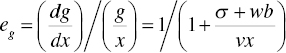 . The degree of the scale elasticity (eg) related to a desirable output is classified by σ and w by the following rule:

Here, it is important to note two concerns regarding Equation (20.1). One of the two concerns is that the parameter v should be strictly positive. In the other case (e.g., zero), it is difficult for us to determine the scale elasticity. That is, if v is zero, then eg becomes zero on a DMU to be examined. Thus, the input‐related dual variable, indicating the slope of a supporting hyperplane, should be positive, not zero, in the measurement of eg. The other concern is that eg is determined by not only σ but also the influence (wb) of the undesirable output. Such an influence on eg cannot be found in the conventional use of DEA, as discussed in Chapter 8, where eg is determined by only σ. Such is the difference between the two approaches.
Next, to describe the scale elasticity (eb) between an input and an undesirable output, let us consider that a supporting hyperplane is – vx – ug+ wb + σ = 0 where the three production factors consist of a single component. Then, we have ![]() and
and ![]() . Consequently, the scale elasticity related to an undesirable output is measured by
. Consequently, the scale elasticity related to an undesirable output is measured by 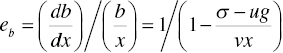 . The scale elasticity (eb) related to an input and an undesirable output is determined by σ and u as follows:

The above classification needs that the input‐related parameter v should be positive. Otherwise, it is difficult for us to measure the scale elasticity related to the undesirable output, as discussed previously. In the case of eb, the type is determined by not only σ but also ug, indicating an influence from a desirable output. This classification rule on ![]() is different from eg. See Equations (20.1) and (20.2).
is different from eg. See Equations (20.1) and (20.2).
Finally, it is important to add two concerns. One of the two concerns is that all parameters for a supporting hyperplane are expressed by dual variables and they are expected to be strictly positive in the elasticity measurement. An exception is σ because it indicates the intercept of a supporting hyperplane. The requirement on dual variables will be changed if we are interested in an occurrence of congestion. See Chapters 21and 23. The other concern is that the concept of “scale elasticity” regarding desirable and undesirable outputs discussed in this section is related to a single desirable output and a single undesirable output. However, the concept of “scale economies” and “scale damages,” which will be discussed in Sections 20.3 and 20.4, are related to multiple desirable and undesirable outputs. These concepts are measured by the proposed formulations for DEA environmental assessment.
20.2.2 Differences between RTS and DTS
Before analytically discussing RTS and DTS in the framework of radial and non‐radial models for DEA environmental assessment, this chapter needs to intuitively explain mathematical similarities and differences as well as their economic implications. They have opposite implications in many economic contexts concerning scale economies and scale damages. See Chapter 8 on scale economies. For example, increasing RTS under natural disposability implies that a unit increase in inputs produces desirable outputs more than their proportional increases without worsening undesirable outputs. This result indicates that, if a DMU increases its operational size, then it becomes more productive on desirable outputs under natural disposability. In this case, a large DMU may outperform small ones in operational performance. Thus, it is recommended that the DMU should increase its operational size to enhance the unified efficiency under natural disposability.
In contrast, in the case of managerial disposability, increasing DTS implies an opposite result in such a manner that a unit increase in inputs yields undesirable outputs more than their proportional increases without worsening desirable outputs. In other words, if a DMU increases its operational size, then it produces more pollution (so, more damage) than before the size increase. Thus, it is recommended that the DMU should decrease its operational size in order to improve the unified efficiency under managerial disposability. The relationship between RTS and DTS, along with corporate strategy on the operational size, is summarized in Table 20.1.
TABLE 20.1 Strategies measured by RTS and DTS
(a) A decrease in undesirable outputs is always the best DTS‐based strategy. The concept of most productive scale size (MPSS), often discussed in the DEA community, may exist in a conventional use of RTS. However, there is no such concept in DTS, corresponding to the MPSS in DEA environmental assessment. The best strategy is to produce no undesirable output. Thus, the concept of MPSS has a very limited implication in DEA environmental assessment. (b) Eco‐technology innovation is essential in reducing an amount of undesirable outputs if a firm has enough capital. If the firm does not have capital accumulation, it must decrease its operation size. See Sueyoshi and Goto (2014a).
| RTS | RTS‐based strategy | DTS | DTS‐based strategy |
| Increasing | It is recommended that a DMU should “increase” the current size. | Increasing | It is recommended that a DMU should “decrease” the current size. As an alternative, it is strongly recommended that the DMU should utilize eco‐technology innovation for environmental protection. |
| Constant | It is recommended that a DMU should “maintain” the current size. | Constant | It is not recommended, but acceptable, that a DMU can “maintain” the current size. As an alternative, it is recommended that the DMU should utilize eco‐technology innovation for environmental protection. |
| Decreasing | It is recommended that a DMU should “decrease” the current size. | Decreasing | It is not recommended, but acceptable, that a DMU can “increase” the current size. |
As summarized in Table 20.1, as an alternative strategy, the type of DTS suggests whether a DMU should introduce eco‐technology innovation within the operation. For example, an increasing DTS indicates that the DMU needs to introduce eco‐technology innovation to enhance its environmental performance. If the DMU has a large amount of capital accumulation, the investment for eco‐technology innovation is more practical than the size reduction in terms of enhancing environmental performance. The implication on increasing DTS may be applied to the case of constant DTS, as well, because it indicates an initial stage of increasing DTS (so, more pollution). In contrast, the eco‐technology innovation may be less important in the case of decreasing DTS because a size increase in inputs less proportionally produces undesirable outputs.
20.3 NON‐RADIAL APPROACH
20.3.1 Scale Economies and RTS under Natural Disposability
Returning to Chapter 16, we can find the following complementary slackness conditions (CSCs) between Models (16.6) and (16.9) on optimality:
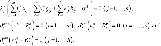
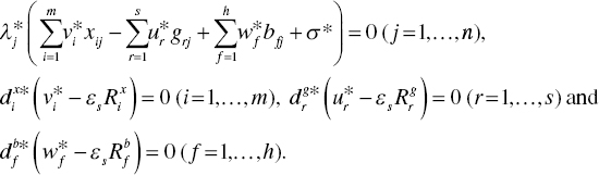
For the first step to determine the type of RTS, this chapter needs to specify the location of a supporting hyperplane in the case where the three production factors have multiple components because the hyperplane is directly related to identifying the RTS measurement. Analytically, a supporting hyperplane(s) of the k‐th DMU under natural disposability is expressed by ![]() , where dual variables, vi (i = 1,…,m), ur (r = 1,…,s) and wf (f = 1,…,h), are parameters for indicating the direction of a supporting hyperplane(s) and σ indicates an intercept of the supporting hyperplane. The parameters are all unknown. Therefore, it is necessary to determine them by the following equation:
, where dual variables, vi (i = 1,…,m), ur (r = 1,…,s) and wf (f = 1,…,h), are parameters for indicating the direction of a supporting hyperplane(s) and σ indicates an intercept of the supporting hyperplane. The parameters are all unknown. Therefore, it is necessary to determine them by the following equation:
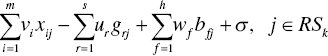
where RSk stands for a reference set of the k‐th DMU whose performance is measured by Model (16.6).
It is important to remind that Section 20.2 specifies the supporting hyperplane by vx – ug + wb + σ = 0 in the case of a single component of the three production factors. Meanwhile, Equation (20.4) specifies the hyperplane as ![]() in the case of their multiple components. Equation (20.4) can be easily obtained from the first group of CSCs, or Equations (20.3).
in the case of their multiple components. Equation (20.4) can be easily obtained from the first group of CSCs, or Equations (20.3).
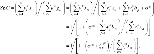
The concept of “scale economies (SEC)” corresponds to the scale electricity (eg) if the three production factors have multiple components. If the k‐th DMU is efficient in unified performance under natural disposability, then the degree of SEC is determined by
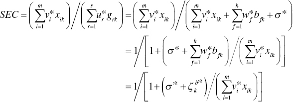
where ![]() . The variable implies an influence from undesirable outputs on the degree of SEC. Equation (20.5) incorporates
. The variable implies an influence from undesirable outputs on the degree of SEC. Equation (20.5) incorporates ![]() in the reformulation, indicating the degree of unified inefficiency in Model (16.9).
in the reformulation, indicating the degree of unified inefficiency in Model (16.9).
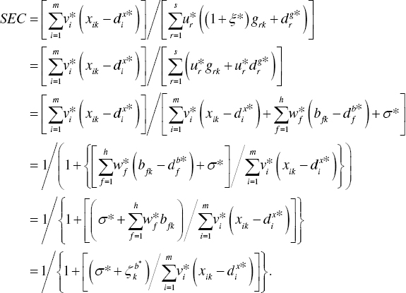
In contrast, if the k‐th DMU is inefficient in unified performance under natural disposability, then the inefficient DMU needs to be projected onto an efficiency frontier. In the case, the degree of SEC can be determined by

Equation (20.6) incorporates ![]()
![]() from the optimal objective value of Models (16.6) and (16.9). The reformulation in Equation (20.6) has three assumptions. First, the inefficient DMU has positive slacks on all production factors so that
from the optimal objective value of Models (16.6) and (16.9). The reformulation in Equation (20.6) has three assumptions. First, the inefficient DMU has positive slacks on all production factors so that ![]() for all i,
for all i, ![]() for all r and
for all r and ![]() for all f because of CSCs, expressed by Equation (20.3). Second, the observed inputs are larger than their slacks so that their differences are positive. Finally, Equation (20.6) considers
for all f because of CSCs, expressed by Equation (20.3). Second, the observed inputs are larger than their slacks so that their differences are positive. Finally, Equation (20.6) considers ![]() because this chapter is interested in the type of RTS on an efficiency frontier that is mainly determined by inputs and desirable outputs. Hence,
because this chapter is interested in the type of RTS on an efficiency frontier that is mainly determined by inputs and desirable outputs. Hence, ![]() is assumed for all f for our computational tractability, indicating that all slacks related to undesirable outputs are positive but very close to zero on the efficiency frontier. Here, the symbol
is assumed for all f for our computational tractability, indicating that all slacks related to undesirable outputs are positive but very close to zero on the efficiency frontier. Here, the symbol ![]() indicates such closeness between the two parts.
indicates such closeness between the two parts.
Assuming both a unique projection of an inefficient DMU onto an efficiency frontier and a unique reference set for the projected DMU, this chapter determines the upper and lower bounds of the dual variable (σ) and the influence factor (![]() ) from undesirable outputs by using the following model:
) from undesirable outputs by using the following model:

The first additional constraint indicates an influence factor from undesirable outputs. The second one is because the objective function of Model (16.6) equals that of Model (16.9) on optimality.
The upper bound (![]() ) and the lower bound (
) and the lower bound (![]() ) of the objective value are obtained from the maximization and minimization of Model (20.7), respectively. An optimal solution of Models (16.6) and (16.9) is feasible in Model (20.7) and vice versa.
) of the objective value are obtained from the maximization and minimization of Model (20.7), respectively. An optimal solution of Models (16.6) and (16.9) is feasible in Model (20.7) and vice versa.
Based upon these upper and lower bounds, the type of RTS of the k‐th DMU is determined by the following classification:

It is important to note that the surface of an efficiency frontier is a set of piece‐wise linear polygonal faces under variable RTS. Therefore, the constant RTS is defined by ![]() (positive) and
(positive) and ![]() (negative), thus covering the range shaped between decreasing and increasing RTS.
(negative), thus covering the range shaped between decreasing and increasing RTS.
20.3.2 Scale Damages and DTS under Managerial Disposability
To determine the degree and type of DTS under managerial disposability, this chapter describes the concept of scale damages (SDA). The degree of SDA depends upon the efficiency or inefficiency status of the k‐th DMU. If the DMU is efficient, then the degree of SDA is determined as follows:

The optimal condition, or ![]() , of Model (16.15) is incorporated into Equation (20.9) because the optimal objective value becomes zero when the DMU is efficient. All optimal dual variables are obtained from Model (16.15). The new variable
, of Model (16.15) is incorporated into Equation (20.9) because the optimal objective value becomes zero when the DMU is efficient. All optimal dual variables are obtained from Model (16.15). The new variable ![]() is incorporated as an influence factor of desirable outputs in Equation (20.9).
is incorporated as an influence factor of desirable outputs in Equation (20.9).
If the k‐th DMU is inefficient, then the DMU needs to be projected on an efficiency frontier. The degree of SDA can be determined on its projected point. That is,

Following the procedure similar to SEC in the previous subsection, the degree of SDA is reformulated as follows:

Assuming both a unique projection of an inefficient DMU onto an efficiency frontier and a unique reference set for the projected DMU, this chapter can determine the upper and lower bounds of the dual variable (σ) and the influence factor (![]() ) from desirable outputs by using the following model:
) from desirable outputs by using the following model:

The first additional constraint indicates the influence from desirable outputs. The second one is due to the condition that the objective function of Model (16.12) equals that of Model (16.15) on optimality.
The upper bound (![]() ) and the lower bound (
) and the lower bound (![]() ) of the objective value are obtained from the maximization and minimization of Model (20.12), respectively. An optimal solution of Models (16.12) and (16.15) is feasible in Model (20.12) and vice versa.
) of the objective value are obtained from the maximization and minimization of Model (20.12), respectively. An optimal solution of Models (16.12) and (16.15) is feasible in Model (20.12) and vice versa.
Based upon the upper and lower bounds, the type of DTS of the k‐th DMU is determined by the following classification:

20.4 RADIAL APPROACH
20.4.1 Scale Economies and RTS under Natural Disposability
The following CSCs always satisfy between Models (17.5) and (17.7) on optimality:
As discussed in Section 20.3, the location of a supporting hyperplane(s), in the case of multiple components of the three production factors, is directly associated with determining the type and degree of RTS. Analytically, the supporting hyperplane of the k‐th DMU under natural disposability is expressed by ![]() , where dual variables vi (i = 1,…, m), ur (r = 1,…, s) and wf (f = 1,…, h) are parameters for indicating the direction of a supporting hyperplane(s) and σ indicates an intercept of the supporting hyperplane. The parameters are all unknown. Therefore, they need to be determined by the following equations:
, where dual variables vi (i = 1,…, m), ur (r = 1,…, s) and wf (f = 1,…, h) are parameters for indicating the direction of a supporting hyperplane(s) and σ indicates an intercept of the supporting hyperplane. The parameters are all unknown. Therefore, they need to be determined by the following equations:

where RSk stands for a reference set of the k‐th DMU whose performance is measured by Model (17.5). A difference between the radial and non‐radial measures can be found in the second term ![]() of Equations (20.15).
of Equations (20.15).
It is important to note that Section 20.2.1 specifies the supporting hyperplane by vx – ug + wb + σ = 0 in the case of a single component of the three production factors. Meanwhile, Equation (20.15) specifies the supporting hyperplane as ![]() in the case of multiple components of the three production factors. Equation (20.15) can be easily obtained from the first group of CSCs, expressed by Equations (20.14).
in the case of multiple components of the three production factors. Equation (20.15) can be easily obtained from the first group of CSCs, expressed by Equations (20.14).
To measure the degree and type of RTS under natural disposability, this chapter classifies DMUs into two groups based upon their efficiency statuses. If the k‐th DMU is efficient in unified performance under natural disposability, then the degree of SEC for multiple components, corresponding to scale elasticity (eg) related to desirable outputs, is determined by
where ![]() . The variable implies an influence from undesirable outputs on the degree of SEC. Equation (20.16) incorporates
. The variable implies an influence from undesirable outputs on the degree of SEC. Equation (20.16) incorporates ![]() in the reformulation that indicates the status of efficiency in Model (17.7).
in the reformulation that indicates the status of efficiency in Model (17.7).
Meanwhile, if the k‐th DMU is inefficient in unified performance under natural disposability, then the inefficient DMU needs to be projected onto an efficiency frontier. In the case, the degree of SEC can be determined by
In Equation (20.17), ![]()
![]() is obtained from the optimal objective value of Models (17.5) and (17.7). Then, we incorporate
is obtained from the optimal objective value of Models (17.5) and (17.7). Then, we incorporate ![]() in the optimal condition because the k‐th DMU is projected onto the efficiency frontier and it becomes zero.
in the optimal condition because the k‐th DMU is projected onto the efficiency frontier and it becomes zero.
The reformulation in Equation (20.17) has the following three assumptions. First, the inefficient DMU has positive slacks on all production factors so that ![]() for all i,
for all i, ![]() for all r, and
for all r, and ![]() for all f. Second, the observed inputs are larger than their slacks so that their differences are positive. Finally, Equation (20.17) considers
for all f. Second, the observed inputs are larger than their slacks so that their differences are positive. Finally, Equation (20.17) considers ![]() because we are interested in the type of RTS that is mainly determined by inputs and desirable outputs. Hence,
because we are interested in the type of RTS that is mainly determined by inputs and desirable outputs. Hence, ![]() is assumed for all f for our computational tractability, indicating that all slacks related to undesirable outputs are positive but being very close to zero.
is assumed for all f for our computational tractability, indicating that all slacks related to undesirable outputs are positive but being very close to zero.
Assuming both a unique projection of an inefficient DMU onto an efficiency frontier and a unique reference set for the projected DMU, this study can determine the upper and lower bounds of the dual variable (σ) and the influence (![]() ) from undesirable outputs using the following model:
) from undesirable outputs using the following model:

The first additional constraint indicates the influence from undesirable outputs. The second additional constraint is because the objective function of Model (17.5) equals that of Model (17.7) on optimality.
The upper bound (![]() ) and the lower bound (
) and the lower bound (![]() ) of the objective value are obtained from the maximization and minimization of Model (20.18), respectively. An optimal solution of Models (17.5) and (17.7) is feasible in Model (20.18) and vice versa.
) of the objective value are obtained from the maximization and minimization of Model (20.18), respectively. An optimal solution of Models (17.5) and (17.7) is feasible in Model (20.18) and vice versa.
Based upon these upper and lower bounds, the type of RTS of the k‐th DMU is determined by the following classification:

20.4.2 Scale Damages and DTS under Managerial Disposability
Shifting our research interest from natural disposability to managerial disposability, where the first priority is environmental performance and the second priority is operational performance, this chapter determines SDA and DTS by the following manner: If the k‐th DMU is efficient in unified efficiency under managerial disposability, then the degree of SDA can be determined by
where ![]() . The variable implies the influence of desirable outputs on SDA.
. The variable implies the influence of desirable outputs on SDA.
Following the reformulation, similar to Equation (20.17), as discussed for SEC, if the k‐th DMU is inefficient in unified efficiency under managerial disposability, then the degree of SDA can be determined by

Assuming both a unique projection of an inefficient DMU onto an efficiency frontier and a unique reference set for the projected DMU, this chapter can determine the upper and lower bounds of the dual variable (σ) and the influence (![]() ) from desirable outputs by the following model:
) from desirable outputs by the following model:

The upper bound (![]() ) and the lower bound (
) and the lower bound (![]() ) of the objective value are obtained from the maximization and minimization of Model (20.22), respectively. An optimal solution of Models (17.10) and (17.12) is feasible in Model (20.22) and vice versa.
) of the objective value are obtained from the maximization and minimization of Model (20.22), respectively. An optimal solution of Models (17.10) and (17.12) is feasible in Model (20.22) and vice versa.
Based upon these upper and lower bounds, the type of DTS of the k‐th DMU is determined by the following classification:

Here, it is important to note two concerns. One of the two concerns is that the type of RTS under radial and non‐radial models may be determined by dropping the influence factor (![]() ) from undesirable outputs. In a similar manner, the type of DTS is determined without the influence factor (
) from undesirable outputs. In a similar manner, the type of DTS is determined without the influence factor (![]() ) from desirable outputs. The determination may be mainly measured by only the dual variable (σ*) that indicates the intercept of a supporting hyperplane. Such is just an approximation (i.e., quick and easy) method that may have computational practicality. The other concern is that this chapter assumes the uniqueness on a projection to an efficiency frontier and a reference set on the frontier. It is true that such an assumption may not be satisfied in the reality of DEA applications. In the case, it is necessary for us to incorporate SCSCs in the proposed approach to determine the type of RTS and DTS as discussed in Chapter 7.
) from desirable outputs. The determination may be mainly measured by only the dual variable (σ*) that indicates the intercept of a supporting hyperplane. Such is just an approximation (i.e., quick and easy) method that may have computational practicality. The other concern is that this chapter assumes the uniqueness on a projection to an efficiency frontier and a reference set on the frontier. It is true that such an assumption may not be satisfied in the reality of DEA applications. In the case, it is necessary for us to incorporate SCSCs in the proposed approach to determine the type of RTS and DTS as discussed in Chapter 7.
20.5 JAPANESE CHEMICAL AND PHARMACEUTICAL FIRMS
This chapter applies the proposed radial approach to assess the unified performance of Japanese chemical and pharmaceutical firms, both of which are included in the chemical industry under a general classification. Due to a page limit, we do not discuss the results on the non‐radial approach in this chapter. Including rubber and plastic products, the total shipment value of the chemical industry, as a whole, amounted to 40 trillion yen in 2010. This value accounted for 13.9% of the entire Japanese manufacturing industry and has increased 1.07 times since 1990. The number of employees in the industry was approximately 880,000 in 2010, which accounted for 11.5% in the entire manufacturing industry. The industry’s operating profit margin remained high, compared to the other manufacturing industries. The plant investment by the industry accounted for 11.6% of all manufacturing industries. All the numbers indicate that the chemical industry plays an important role for Japanese economy. See the information source that provides a detailed description on Japanese chemical industry.
The Japanese chemical industry was the third largest in global chemical shipments with US$ 338.2 billion in 2010 after China and the United States. However, the size of each company was small, compared to the other world‐class chemical companies. Currently, the production activities of these chemical firms produce various environmental problems, so that the Japanese government requires them to pay serious attention to the global warming and climate change and to reduce the amount of chemical substances. For example, the industry is the second largest emitter of CO2 in Japan following the steel industry, after allocating the amount of the industry’s indirect emissions. Thus, environmental consideration such as improved energy efficiency and environmental protection is an important business concern for the chemical industry. The total amount of energy is treated as an input in this chapter to incorporate the influence of such energy consumption on their unified efficiency measures. The tradeoff between business prosperity and environmental protection is very important for the industry, so indicating the research importance of this study. See Chapter 14 on the history of Japanese environmental issue.
In examining the unified efficiency measures of chemical firms, this chapter compares performance between two sub‐samples: pharmaceutical firms and the other chemical firms, because they have business similarities and both are classified as the chemical industry in a broad sense. The data set contains 31 Japanese chemical and pharmaceutical firms and it consists of four inputs: the amount of total assets (unit: million yen), the number of employees, the total amount of energy inputs (unit: Giga joule), and the total cost for environmental protection (unit: million yen) in order to produce a desirable output: total sales (unit: million yen), along with two undesirable outputs: the total amount of greenhouse gas emissions (unit: ton of CO2) and the total amount of waste discharges (unit: ton). The observed annual periods were from 2007 to 2010.
Data Accessibility:
Toyo Keizai Inc. has published the total amount of energy inputs, the total cost for environmental protection, the total amount of greenhouse gas emissions and the total amount of waste discharges. Other production factors have been obtained from Nippon Keizai Shinbun Inc.
This chapter selects representative companies in the chemical industry which provide all the necessary data from 2007 to 2010. Thus, the data set used for this chapter is structured in a balanced panel data that consists of 31 firms over these four years.
To measure the unified efficiency measures and the type of RTS and DTS in these firms, this chapter first pools all data sets together and treats it as a cross‐sectional data. Then, this chapter applies the proposed radial approach to the pooled data set.
The research of Sueyoshi and Goto (2014a) recorded that pharmaceutical firms outperformed chemical firms in terms of their average unified efficiency measures under natural and managerial disposability. This result implies that the former firms pay more attention to their operational and environmental performance than the latter firms.
As an extension of their work, Table 20.2 summarizes the upper bound (![]() ) and the lower bound (
) and the lower bound (![]() ) of 31 firms, both of which are obtained from Model (20.18). These upper and lower bounds determine the type of RTS. As listed at the bottom of Table 20.2, 28.6%, 23.8% and 47.6% of the chemical firms, respectively, exhibit increasing, constant and deceasing RTS. Meanwhile, 5.0%, 40.0% and 55.0% of the pharmaceutical firms exhibit increasing, constant and deceasing RTS. The two results imply that approximately 50% of firms (i.e., 47.6% of the chemical firms and 55.0% of the pharmaceutical firms) in the two groups of firms should reduce their corporate sizes to enhance their operational performance.
) of 31 firms, both of which are obtained from Model (20.18). These upper and lower bounds determine the type of RTS. As listed at the bottom of Table 20.2, 28.6%, 23.8% and 47.6% of the chemical firms, respectively, exhibit increasing, constant and deceasing RTS. Meanwhile, 5.0%, 40.0% and 55.0% of the pharmaceutical firms exhibit increasing, constant and deceasing RTS. The two results imply that approximately 50% of firms (i.e., 47.6% of the chemical firms and 55.0% of the pharmaceutical firms) in the two groups of firms should reduce their corporate sizes to enhance their operational performance.
TABLE 20.2 Returns to scale
(a) Source: Sueyoshi and Goto (2014a). (b) I, C and D stand for increasing, constant and decreasing RTS, respectively. (c) Max. and Min. indicate the upper and lower bounds of Model (20.18).
| No. | Year | 2007 | 2008 | 2009 | 2010 | ||||||||
| Company Name | Max | Min | Type of RTS | Max | Min | Type of RTS | Max | Min | Type of RTS | Max | Min | Type of RTS | |
| 1 | Kuraray | 0.2657 | 0.2657 | D | 0.3242 | 0.3242 | D | 0.3065 | 0.3065 | D | 0.0799 | 0.0799 | D |
| 2 | Asahi‐Kasei | –2.1553 | –2.1553 | I | –0.1114 | –0.1114 | I | 0.9593 | 0.9593 | D | 0.9763 | 0.9763 | D |
| 3 | Sumitomo Chemical Company | 1.1027 | 1.1027 | D | 1.0685 | 1.0685 | D | 1.1782 | 1.1782 | D | 1.0915 | 1.0915 | D |
| 4 | Tosoh | 0.2046 | –0.2148 | C | 0.0442 | 0.0442 | D | 0.1008 | 0.1008 | D | 0.0477 | 0.0477 | D |
| 5 | Tokuyama Corporation | 0.0053 | 0.0053 | D | 0.0052 | 0.0052 | D | 0.6460 | 0.6460 | D | 0.6447 | 0.6447 | D |
| 6 | Toagosei | 0.1335 | 0.1335 | D | –0.0740 | –0.0740 | I | –0.0851 | –0.0851 | I | –0.3053 | –0.3053 | I |
| 7 | Taiyo Nippon Sanso | 0.3645 | –0.7341 | C | 0.1232 | –0.5504 | C | –0.2891 | –0.2891 | I | –0.5691 | –0.5691 | I |
| 8 | Mitsui Chemicals | 0.9941 | –0.0502 | C | 0.0322 | 0.0322 | D | 0.4643 | 0.4643 | D | 0.4202 | 0.4202 | D |
| 9 | JSR | 0.0963 | 0.0963 | D | 0.1228 | 0.1228 | D | 0.1469 | 0.1469 | D | 0.1487 | 0.1487 | D |
| 10 | Tokyo Ohka Kogyo | –0.1179 | –0.1179 | I | –0.0814 | –0.0814 | I | –0.2965 | –0.2965 | I | –0.1612 | –0.1612 | I |
| 11 | Sekisui | 0.2852 | –0.0981 | C | 0.1036 | –0.1163 | C | 0.0185 | 0.0185 | D | 0.0061 | –0.1797 | C |
| 12 | Takiron | –0.2972 | –0.2972 | I | –0.2900 | –2.3289 | I | –0.2490 | –7.1154 | I | –0.1732 | –913.7409 | I |
| 13 | Hitachi Chemical | 0.3884 | –0.0349 | C | 0.1665 | 0.1665 | D | 0.2073 | 0.2073 | D | 0.2562 | –0.0501 | C |
| 14 | Nippon Kayaku | 0.0206 | –0.2459 | C | 0.1027 | 0.1027 | D | 0.0983 | 0.0983 | D | 0.0950 | 0.0950 | D |
| 15 | ADEKA | 0.8771 | –12.5532 | C | 0.0922 | 0.0922 | D | 0.0796 | 0.0796 | D | 0.0779 | 0.0779 | D |
| 16 | Sanyo Chemical Industries | 0.1210 | 0.1210 | D | 0.1240 | 0.1240 | D | 0.1418 | 0.1418 | D | 0.1327 | 0.1327 | D |
| 17 | Takeda Pharmaceutical Company | 0.9872 | –0.0872 | C | 0.9505 | –0.1137 | C | 0.9678 | –0.1163 | C | 0.9492 | –0.0712 | C |
| 18 | Astellas | 0.5544 | 0.5544 | D | 0.2480 | 0.2480 | D | 0.2946 | –0.0092 | C | 0.2440 | 0.2440 | D |
| 19 | Shionogi & Co. | 0.4644 | 0.4644 | D | 0.6310 | 0.6310 | D | 0.5743 | 0.5743 | D | 0.5156 | 0.5156 | D |
| 20 | Nippon Shinyaku | 0.2768 | 0.2768 | D | 0.3666 | –41.8633 | C | 0.4420 | –3.8724 | C | 0.4026 | –0.8512 | C |
| 21 | Chugai Pharmaceutical Co. | 0.7796 | –0.0565 | C | 0.5598 | 0.5598 | D | 0.7159 | –0.1570 | C | –0.0294 | –0.0294 | I |
| 22 | Eisai | 0.3155 | 0.3155 | D | 0.2116 | 0.2116 | D | 0.6646 | 0.1591 | D | 0.5347 | –0.1248 | C |
| 23 | Ono Pharmaceutical Co. | 0.6018 | –0.5896 | C | 0.5690 | –0.5402 | C | 0.3505 | 0.3505 | D | 0.5114 | 0.2259 | D |
| 24 | Tsumura & Co. | 0.0265 | 0.0265 | D | 0.0256 | 0.0256 | D | 0.0254 | 0.0254 | D | 0.0203 | 0.0203 | D |
| 25 | Kissei Pharmaceutical Co. | –1.8733 | –1.8733 | I | 0.5243 | –1.2030 | C | 0.3724 | –5.2633 | C | 0.5959 | –53.9556 | C |
| 26 | Daiichi Sankyo Co. | 0.5474 | 0.5474 | D | 0.5436 | 0.5436 | D | 0.5512 | 0.5512 | D | 0.4951 | 0.4951 | D |
| 27 | Nippon Paint | 0.6822 | –4.4053 | C | –0.0583 | –0.3759 | I | –0.1387 | –0.1387 | I | 0.0947 | –0.9554 | C |
| 28 | DIC | 0.1633 | 0.1633 | D | 0.1641 | 0.1641 | D | 0.9403 | –2.2286 | C | 0.6418 | –15.8280 | C |
| 29 | Shiseido | 0.6330 | –0.3238 | C | 0.6029 | –0.2516 | C | –0.0422 | –0.2301 | I | 0.6219 | –0.2727 | C |
| 30 | T. Hasegawa Co. | –0.7621 | –5.2836 | I | –1.0704 | –1.0704 | I | –0.9781 | –6.6281 | I | –1.0511 | –1.0511 | I |
| 31 | Arakawa Chemical Industries | 0.1578 | –1.6944 | C | 0.1502 | –5.1439 | C | –0.1640 | –0.1640 | I | –0.1953 | –0.1953 | I |
| Chemical firms | I | C | D | ||||||||||
| 28.6% | 23.8% | 47.6% | |||||||||||
| Pharmaceutical firms | I | C | D | ||||||||||
| 5.0% | 40.0% | 55.0% | |||||||||||
Table 20.3 summarizes the upper bound (![]() ) and lower bound (
) and lower bound (![]() ) of these firms, both of which are obtained from Model (20.22). These upper and lower bounds determine the type of DTS. The type of DTS, summarized in Table 20.3, is different from the type of RTS of Table 20.2. As listed at the bottom of Table 20.3, 59.5%, 8.3% and 32.1% of the chemical firms, respectively, exhibit increasing, constant and deceasing DTS. The result implies that 59.5% of chemical firms should reduce their sizes. As an alternative strategy, it is necessary for them to introduce new environmental technology for reducing their undesirable outputs. Meanwhile, 37.5%, 37.5% and 25.0% of the pharmaceutical firms exhibit increasing, constant and deceasing DTS. This result indicates that environmental strategy may depend upon each pharmaceutical firm.
) of these firms, both of which are obtained from Model (20.22). These upper and lower bounds determine the type of DTS. The type of DTS, summarized in Table 20.3, is different from the type of RTS of Table 20.2. As listed at the bottom of Table 20.3, 59.5%, 8.3% and 32.1% of the chemical firms, respectively, exhibit increasing, constant and deceasing DTS. The result implies that 59.5% of chemical firms should reduce their sizes. As an alternative strategy, it is necessary for them to introduce new environmental technology for reducing their undesirable outputs. Meanwhile, 37.5%, 37.5% and 25.0% of the pharmaceutical firms exhibit increasing, constant and deceasing DTS. This result indicates that environmental strategy may depend upon each pharmaceutical firm.
TABLE 20.3 Damages to scale
(a) Source: Sueyoshi and Goto (2014a). (b) I, C and D stand for increasing, constant and decreasing DTS, respectively. (c) Max. and Min. indicate the upper and lower bounds of Model (20.22).
| No. | Year | 2007 | 2008 | 2009 | 2010 | ||||||||
| Company Name | Max | Min | Type of DTS | Max | Min | Type of DTS | Max | Min | Type of DTS | Max | Min | Type of DTS | |
| 1 | Kuraray | 0.2171 | 0.2171 | I | 0.2366 | 0.2366 | I | 0.2430 | 0.2430 | I | 0.2367 | 0.2367 | I |
| 2 | Asahi‐Kasei | 4.9969 | 4.1855 | I | 66.5688 | –0.0447 | C | 0.0451 | 0.0451 | I | 0.0464 | 0.0464 | I |
| 3 | Sumitomo Chemical Company | 25.5812 | 0.1970 | I | 1.2689 | 0.5734 | I | 0.4082 | 0.4082 | I | 2.6965 | 0.0444 | I |
| 4 | Tosoh | 0.0175 | 0.0175 | I | 0.0364 | 0.0364 | I | 0.0365 | 0.0365 | I | 0.0349 | 0.0349 | I |
| 5 | Tokuyama Corporation | 0.0337 | 0.0337 | I | 0.0355 | 0.0355 | I | 0.0379 | 0.0379 | I | 0.0389 | 0.0389 | I |
| 6 | Toagosei | 0.1255 | 0.1255 | I | 1.5891 | 0.1758 | I | 0.5955 | 0.1044 | I | 0.1965 | 0.1965 | I |
| 7 | Taiyo Nippon Sanso | 2.8671 | –0.1710 | C | 2.6864 | –0.0788 | C | 0.5576 | 0.5576 | I | 3.5516 | 0.4821 | I |
| 8 | Mitsui Chemicals | 5.0876 | –0.1251 | C | 0.2701 | 0.0450 | I | 2.2791 | 0.3123 | I | 1.6088 | 0.0068 | I |
| 9 | JSR | 0.2988 | 0.2988 | I | 0.5582 | 0.5582 | I | 0.4740 | 0.4740 | I | 0.4380 | 0.4380 | I |
| 10 | Tokyo Ohka Kogyo | –0.2329 | –0.2329 | D | –0.2431 | –0.2431 | D | –0.2467 | –0.2467 | D | –0.2597 | –0.2597 | D |
| 11 | Sekisui | 7.6427 | 0.2580 | I | 4.5479 | 0.3013 | I | 8.4312 | 0.5311 | I | 0.9649 | 0.9649 | I |
| 12 | Takiron | –0.0490 | –0.0490 | D | –0.0548 | –0.0548 | D | –0.3452 | –0.3452 | D | –0.3685 | –0.3685 | D |
| 13 | Hitachi Chemical | 1.6540 | 1.6540 | I | 1.8062 | 1.8062 | I | 1.7153 | 1.7153 | I | 1.8216 | 1.8216 | I |
| 14 | Nippon Kayaku | –0.1328 | –0.1328 | D | –0.1001 | –0.1001 | D | –0.1247 | –0.1247 | D | –0.1223 | –0.1223 | D |
| 15 | ADEKA | 80.8672 | –0.9991 | C | 0.1503 | 0.1503 | I | –0.0202 | –0.0202 | D | –0.0378 | –0.0378 | D |
| 16 | Sanyo Chemical Industries | 0.7882 | 0.7882 | I | 0.3380 | 0.3380 | I | 0.3442 | 0.3442 | I | 0.9126 | 0.9126 | I |
| 17 | Takeda Pharmaceutical Company | 19.5288 | –0.0801 | C | 0.4972 | –0.1159 | C | 3.7713 | –0.4342 | C | 28.5277 | –0.4838 | C |
| 18 | Astellas | 0.5524 | 0.5524 | I | 0.3837 | 0.3837 | I | 0.9291 | 0.3824 | I | 0.7968 | 0.7968 | I |
| 19 | Shionogi & Co. | 1.0761 | 1.0761 | I | 1.1331 | 1.1331 | I | 1.0724 | 1.0724 | I | 1.1271 | 1.1271 | I |
| 20 | Nippon Shinyaku | –0.5162 | –0.5162 | D | –0.6310 | –0.6310 | D | 0.2010 | –0.9994 | C | 0.3054 | –0.2873 | C |
| 21 | Chugai Pharmaceutical Co. | 9.2419 | –0.5722 | C | 18.3903 | –0.3579 | C | 1.6448 | –0.4788 | C | 0.8475 | 0.8475 | I |
| 22 | Eisai | 18.3530 | 4.4302 | I | –0.2861 | –0.2861 | D | 30.3043 | –0.4729 | C | 12.3657 | –0.4714 | C |
| 23 | Ono Pharmaceutical Co. | 2.7906 | –0.5797 | C | 3.4447 | –0.9989 | C | 1.3170 | –0.1574 | C | 2.2281 | –0.5970 | C |
| 24 | Tsumura & Co. | 0.0071 | 0.0071 | I | –0.1634 | –0.1634 | D | –0.0734 | –0.0734 | D | –0.1711 | –0.1711 | D |
| 25 | Kissei Pharmaceutical Co. | –0.4758 | –0.4758 | D | –0.9009 | –0.9009 | D | –0.9033 | –0.9033 | D | –0.4981 | –0.4981 | D |
| 26 | Daiichi Sankyo Co. | 19.3410 | 0.9919 | I | 1.4865 | 1.4865 | I | 3.1658 | 1.2318 | I | 4.5196 | 0.5157 | I |
| 27 | Nippon Paint | 14.2178 | –0.5438 | C | –0.3302 | –0.3302 | D | –0.3564 | –0.3564 | D | –0.3727 | –0.3727 | D |
| 28 | DIC | 21.8292 | 0.3856 | I | 21.4282 | 0.4443 | I | 0.8378 | 0.8378 | I | 17.7840 | 0.5498 | I |
| 29 | Shiseido | –0.2859 | –0.2859 | D | –0.4029 | –0.4029 | D | 1.2788 | 1.2788 | I | 6.5949 | –0.5371 | C |
| 30 | T. Hasegawa Co. | –0.2777 | –0.2777 | D | –0.3264 | –0.3264 | D | –0.3602 | –0.3602 | D | –0.3212 | –0.3212 | D |
| 31 | Arakawa Chemical Industries | –0.0705 | –0.0705 | D | –0.0786 | –0.0786 | D | –0.0917 | –0.0917 | D | –0.0711 | –0.0711 | D |
| Chemical firms | I | C | D | ||||||||||
| 59.5% | 8.3% | 32.1% | |||||||||||
| Pharmaceutical firms | I | C | D | ||||||||||
| 37.5% | 37.5% | 25.0% | |||||||||||
20.6 SUMMARY
This chapter described how to determine the type of RTS under natural disposability and the type of DTS under managerial disposability by using both radial and non‐radial models. The proposed DEA approach incorporated strategic concepts on natural or managerial disposability, discussed in Chapter 15, into the proposed computational process. The proposed measurement provided us with empirical evidence on both the operational size of each DMU and how to guide its environmental strategy by eco‐technology innovation on undesirable outputs.
As an application, this chapter compared between Japanese chemical and pharmaceutical firms by their measures on RTS and DTS. This chapter identified two empirical findings. One of the two findings was that approximately 50% of firms (i.e., 47.6% of the chemical firms and 55.0% of the pharmaceutical firms) in the two groups should reduce their corporate sizes to enhance their operational performance. The other finding was that 59.5% of chemical firms should reduce their sizes to enhance their environmental performance. As an alternative strategy, it is recommended that they could introduce new environmental technology for reducing their undesirable outputs. Since Japanese chemical firms are relatively small in the global market, the resulting type of classification on RTS and DTS may become different if this chapter incorporates foreign firms (e.g., corporations in China, the United States and European nations) in the data sample used in this study. Therefore, although it is recommended in this chapter that the scale reduction for Japanese chemical and pharmaceutical firms, it does not immediately imply that they need to reduce their operation sizes in the global market. Rather, we recommend the introduction of eco‐technology innovation for improving their energy and environment performance as well as to increase their operational performance.