
25
COMMON MULTIPLIERS
25.1 INTRODUCTION
Returning to Chapter 7 (on SCSCs) and Chapter 11 (on DEA‐DA), this chapter1 discusses how to evaluate the performance of Japanese electric power companies by the combined use of DEA/SCSCs with DEA‐DA. Here, DEA/SCSCs implies DEA equipped with SCSCs.
This chapter discusses their performance assessment only under natural disposability so that we can exclude the undesirable outputs from the proposed application. This type of DEA application often exists in the assessment of an electric power industry. For example, renewable energy sources (e.g., solar and wind) and nuclear power do not produce GHGs such as CO2 when they generate electricity. Therefore, many people are interested in the full use of renewable energy. As an extension of Chapters 7 and 11, this chapter documents DEA assessment for ranking analysis whose result contains a single efficient DMU and the remaining others are inefficient.
From the perspective of DEA, the purpose of this chapter is to document how to overcome the following five difficulties, all of which are widely observed in its applications in energy sectors.
- Reducing the number of many efficient DMUs: A difficulty of DEA applications is that they usually produce many efficient DMUs in terms of operational efficiency (OE). For example, 90% of DMUs become efficient and the remaining 10% are inefficient. The result is mathematically acceptable, but managerially problematic, because of so many efficient DMUs. This type of problem often occurs when many multipliers (i.e., dual variables) become zero on optimality. The occurrence of zero in multipliers implies that DEA does not fully utilize information on production factors in a data set, even if we use them as inputs and desirable outputs. To reduce the number of efficient DMUs, previous studies proposed various types of multiplier restrictions such as assurance region (AR) analysis (Thompson et al., 1986)2 and cone ratio (CR) approach (Charnes et al., 1989)3 as discussed in Chapter 4. See also Chapters 22 and 23 on a different type of multiplier restrictions, referred to as “explorative analysis.” The multiplier restrictions proposed in the previous studies often needed prior information, such as previous experience and empirical fact, to restrict multipliers in a specific range that fits with our expectation. A practical problem is that it is often difficult for us to access such prior information. As a result, DEA users have a difficulty in using conventional multiplier restrictions in a prescribed range as they expect. Furthermore, even if we can access such prior information, the multiplier restriction approaches (e.g, AR and CR) do not guarantee that DEA can always produce positive multipliers. In the worst case, they may produce an infeasible solution because of strict restriction on multipliers.
- Multiple Projections and Multiple Reference Sets: DEA often suffers from an occurrence of multiple projections and multiple reference sets. To overcome the difficulty, Sueyoshi and Sekitani (2007a, b, 2009)4–6 theoretically discussed the use of DEA combined with SCSCs. See Chapter 7 for a detailed discussion on SCSCs. They also discussed the occurrence of multiple reference sets and multiple projections that became very problematic in the measurement of RTS. See Chapter 8 on RTS. To deal with such a problem, their studies proposed the use of DEA/SCSCs. The use of SCSCs mathematically guarantees that it usually produces positive multipliers on efficient firms. However, the use of DEA/SCSCs does not guarantee that it can always reduce the number of efficient firms as required above.
- Common Multipliers: A conventional use of DEA cannot provide an industry‐wide evaluation by common multipliers (weights). Rather, it evaluates each DMU by relatively comparing its performance with efficient firms belonging to a reference set. Thus, DEA provides a limited scope on performance evaluation by paying attention to only efficient DMUs in a reference set. The performance evaluation, which we deal with in this chapter, expects the DEA result which contains a single efficient DMU and the remaining other inefficient ones. This type of research is necessary for performance assessment. For example, corporate leaders and policy makers usually do not care about the magnitude of efficiency scores on their organizations (i.e., DMUs). Rather, they do care about the rank of their organizations within their industries. Thus, it is important for us to discuss how to rank all DMUs by an industry‐wide assessment based upon common multipliers (weights). For such a purpose, this chapter proposes the use of DEA/SCSCs combined with DEA‐DA.
- Statistical Inference: A difficulty, even in a combined use between DEA/SCSCs and DEA‐DA, is that they do not have any statistical inference. That is a methodological drawback of DEA, compared with statistics and econometrics. After obtaining the efficiency scores of all DMUs, this chapter describes a use of a rank sum test to examine null hypotheses based upon their efficiency‐based ranks. The combined use between DEA/SCSCs and DEA‐DA, along with a rank sum test, may provide a new type of performance assessment and its related analytical capability. See Chapter 17 on the two rank sum tests (i.e., Mann–Whitney and Kruskal–Wallis rank sum tests).
- Efficiency Requirement: An efficiency score should locate between zero and one, where “zero” implies full inefficiency and “one” implies full efficiency. However, many DEA models such as radial and non‐radial models, as discussed in Chapter 6, do not satisfy the efficiency requirement. Exceptions are RAM, SBM and Russell measures. See Chapter 6 for mathematical proof on the claim. This chapter discusses how the newly proposed approach can obtain such efficiency scores with the efficiency requirement.
The remainder of this chapter has the following structure: Section 25.2 visually describes the computational structure of the proposed approach. Section 25.3 describes an analytical linkage between DEA/SCSCs and DEA‐DA. Section 25.4 describes a computational procedure concerning how to rank all DMUs and how to apply a rank sum test. Section 25.5 documents an illustrative example related to Japanese electric power industry. Section 25.6 provides a summary on this chapter.
25.2 COMPUTATIONAL FRAMEWORK
Figure 25.1 depicts a computational flow of the proposed approach. As mentioned previously, DEA usually produces many efficient DMUs because of many zeros in their multipliers (dual variables). Therefore, it is necessary for us to examine whether the type of difficulty occurs or not in DEA results. If the problem occurs, the proposed approach starts combining between primal and dual models in such a manner that the combination satisfies SCSCs and it may yield positive multipliers on efficient DMUs.

FIGURE 25.1 Computational flow of proposed approach (a) The incorporation of SCSCs into DEA is not necessary if the primal model incorporates data range adjustments on slacks, as found in radial and non‐radial measurements proposed by DEA environmental assessment. See Chapters in Section II. They can always produce positive multipliers (i.e., dual variables) so that the environmental assessment discussed in this book can fully utilize all production factors. Hence, the proposed approaches can omit the computational part on DEA/SCSCs and starts from the DMU classification by DEA‐DA. A problem is that the subjectivity of a user may be included in the range adjustments. The use of SCSCs can avoid such a difficulty related to a conventional use of DEA. See Chapter 7 on the use of SCSCs.
After the combination, the proposed approach needs to classify all DMUs into operationally efficient and inefficient groups by DEA/SCSCs. Then, we apply DEA‐DA to identify common multipliers on production factors. Using the rank of all DMUs based upon their efficiency measures, we can conduct a rank sum test to examine a null hypothesis regarding whether multiple groups or periods have a same distribution or not on their efficiency measures.
25.3 COMPUTATIONAL PROCESS
First, this chapter returns to Model (7.9) in Chapter 7 that proposed the following radial model equipped with SCSCs:

Since Chapter 7 describes Model (25.1) in detail, this chapter does not describe its unique features, here. However, the following two concerns are important for discussing the analytical feature of SCSCs from environmental assessment. One of the two concerns is that Model (25.1) does not incorporate undesirable outputs, as mentioned in chapters in Section II. It is not difficult for us to extend Model (25.1) into the environmental assessment that incorporates undesirable outputs within the computational framework. The other concern is that Model (25.1) does not incorporate εs because the small number is not necessary under the use of SCSCs. That is a purpose of SCSCs in DEA. All chapters, except this chapter, in Section II incorporate the data range adjustments on slacks in the objective function of formulations. In the case, the SCSCs are also not necessary because they always produce positive multipliers (i.e., dual variables). See Chapters 22 and 23 that extend the multiplier restriction into “exploration analysis” by which all multipliers are always positive, so belonging to our expected ranges without any prior information.
Mathematical Rationale on DEA/SCSCs:
Model (25.1) has methodological strengths and drawbacks. Table 25.1 compares DEA with DEA/SCSCs. Chapter 7 did not summarize such differences. As mentioned in Chapter 7, DEA often suffers from an occurrence of multiple reference sets and multiple projections. Model (25.1) can deal with such difficulties (i.e., multiple solutions) on efficient DMUs, but it does not directly solve the occurrence of multiple reference sets and multiple projections on inefficient DMUs. An important feature of Model (25.1) is that it can identify a unique reference set, often mathematically referred to as “a minimum face,” that can cover all possible reference sets on an efficiency frontier onto which each inefficient DMU projects. Thus, Model (25.1) can identify a unique reference set on the minimum face for efficient DMUs. Moreover, even if multiple projections occur on an inefficient DMU, DEA/SCSCs can specify their projection ranges onto the minimum face. Thus, DEA/SCSCs can solve the uniqueness issue on inefficient DMUs by a projection onto the minimum face.
TABLE 25.1 Differences between DEA and DEA/SCSCs
| DEA | DEA/SCSCs | |
| Sign of multipliers (dual variables) | Multipliers may be positive or zero in their signs. The sign of many multiples is often zero. The occurrence of zero in multipliers implies that DEA evaluation does not utilize information on all production factors. Hence, the conventional use of DEA restricts multipliers by a non‐Archimedean small number. | All multipliers of efficient DMUs are always positive in their signs in Model (25.1). The assessment by DEA/SCSCs can fully utilize information on all production factors. |
| Multiplier restriction | DEA needs multiplier restriction methods such as CR and AR. Such multiplier restriction methods proposed in the conventional DEA studies do not guarantee that all multipliers are always positive. | Model (25.1) does not need any multiplier restriction method. |
| Prior information | Multiplier restriction methods proposed in the previous DEA studies need prior information (e.g., experience) for the restriction. Consequently, the restriction is subjective so that different individuals use different restrictions, so producing different results on DEA performance assessment. | Model (25.1) restricts multipliers based upon the mathematical property of SCSCs. Consequently, the restriction is unique, not depending upon prior information. |
| Multiple reference sets and multiple projections | DEA often suffers from an occurrence of multiple reference sets and multiple projections. | Model (25.1) can uniquely identify a single reference set onto which an inefficient DMU is projected. |
| Reduction in the number of efficient DMUs | The multiplier restriction methods incorporated into DEA may reduce the number of efficient DMUs. | Model (25.1) cannot reduce the number of efficient DMUs. |
Besides the description in Table 25.1, this chapter considers DEA as an identification process of an efficiency frontier because the efficiency measure of all DMUs is determined by comparing their performance with DMUs on the frontier. The efficiency frontier consists of only DMUs whose efficiency scores are unity and all slacks are zero in radial and non‐radial measurements. The requirement (i.e., zero in all the slacks) is very helpful in understanding the importance of SCSCs. To explain it in detail, let us consider Equations (7.7) and (7.8), which are ![]() for all i = 1,…, m and
for all i = 1,…, m and ![]() for all r = 1,…, s. Since all the efficient DMUs have zero in their slacks, the two groups of equations immediately indicate
for all r = 1,…, s. Since all the efficient DMUs have zero in their slacks, the two groups of equations immediately indicate ![]() for all i and
for all i and ![]() for all r on optimality. Thus, the incorporation of SCSCs implies that multipliers become positive on efficient DMUs.
for all r on optimality. Thus, the incorporation of SCSCs implies that multipliers become positive on efficient DMUs.
The incorporation of SCSCs does not guarantee whether inefficient DMUs have positive multipliers because they have at least one positive slack variable(s). Such a result may not be important in Model (25.1) because inefficient DMUs do not consist of an efficiency frontier. Even if we drop an inefficient DMU(s) from the computation of DEA, such elimination does not influence the whole DEA evaluation of the other DMUs. Furthermore, when DEA projects an inefficient DMU onto an efficiency frontier, the SCSCs restrict its projection in such a manner that all multipliers of the inefficient DMU become positive on the efficiency frontier. Thus, the projection of the inefficient DMU is always restricted on a reduced range, or the minimum face, shaped by the SCSCs.
After classifying all DMUs into efficient and inefficient groups by Model (25.1), the proposed approach identifies a supporting hyperplane between the two groups. Returning to Chapter 8, we can specify the supporting hyperplane by ![]() where
where ![]() and
and ![]() are parameters for indicating the direction of a supporting hyperplane and σ indicates the intercept of the supporting hyperplane. The parameters are all unknown and need to be measured by
are parameters for indicating the direction of a supporting hyperplane and σ indicates the intercept of the supporting hyperplane. The parameters are all unknown and need to be measured by  ,
, ![]() , where RSk stands for a reference set of the k‐th DMU.
, where RSk stands for a reference set of the k‐th DMU.
The above concern implies how the reference set of the k‐th DMU characterizes the location of a supporting hyperplane(s). In the case, the uniqueness of a reference set is important in identifying the supporting hyperplane. Hence, this chapter fully utilizes SCSCs for DEA assessment because of the above mathematical rationale. Moreover, it is possible for us to change the location of the supporting hyperplane to separate efficient and inefficient DMUs as a discriminant hyperplane. Therefore, this chapter needs to describe the locational change of the discriminant hyperplane by using DEA‐DA.
Acknowledging the importance of SCSCs in terms of identifying the supporting hyperplane, this chapter mentions that the proposed use of DEA/SCSCs has still another type of difficulty in reducing the number of efficient DMUs. To deal with the difficulty, this chapter proposes to use the following new approach that is an extended version of previous radial and non‐radial approaches:
- Step 1: Using results from Model (25.1), we classify all DMUs into efficient (E) and inefficient (IE) groups.
- Step 2: Apply the following DEA‐DA model to the two groups (E and IE):
Here, M is a prescribed large number and ε is a prescribed small number. It is necessary for us to prescribe the two numbers before solving Model (25.2). The objective function minimizes the total number of incorrectly classified DMUs by counting a binary variable (μj). In the classification, the efficient DEA group (E) has more priority than the inefficient group (IE). Therefore, Model (25.2) adds M to the efficient group in the objective of Model (25.2). The discriminant score is expressed by
 (
( ) and
) and  (
( ), respectively, after changing their locations from the left hand side to the right hand side of Model (25.2). The sign of σ is not important because it is unrestricted. The small number (ε) is incorporated into the right hand side of Model (25.2) in order to avoid a case where an observation(s) exists on the estimated discriminant function. All the DMUs on desirable outputs and inputs connect to each other by a discriminant function, which we consider as the supporting hyperplane in DEA. Unknown weights vi for i = 1, …, m and ur for r = 1, …, s are determined by the minimization of incorrect classifications. The last two constraints indicate that all the variables (vi for i = 1, …, m, and ur for r = 1, …, s) are positive so that the discriminant function is a full model. Thus, Model (25.2) incorporates the constraints
  to “normalize” weight estimates in the manner that all weights are expressed by a positive percentage and the sum of all weights is unity. Such a change depends upon the degree of freedom between the number of observations and that of weights.
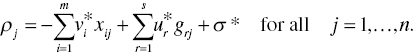
 - Step 3: After applying Model (25.2) to the data set, this chapter obtains an optimal solution and compute the following score for the j‐th DMU:(25.3)
- Step 4: Using the ρj scores, this chapter computes their adjusted efficiency scores by the following procedure:
- Find the maximum and minimum values of ρ by
 and
and  .
. - Find the range between them by
- (b-1) Range (A) =
 if
if  is non‐negative or
 - (b-2) Range (B) =
 if
if  is negative.
- (b-1) Range (A) =
- The adjusted efficiency score for the j‐th DMU is determined by
- (c-1) Efficiency = [
 ]/[range (A)] if
  is non‐negative or
 - (c-2) Efficiency = /[range(B)] if
 is negative.
- (c-1) Efficiency = [
- Find the maximum and minimum values of ρ by

The following five concerns are important in describing the combined use between DEA‐DA and DEA/SCSCs. First, Figure 25.2 visually describes the relationship between a supporting line obtained from Model (25.1) and a discriminant line determined by Model (25.2). The figure contains three efficient DMUs and the remaining inefficient DMUs. The symbol ○ stands for an efficient DMU and the symbol × stands for an inefficient DMU. For our visual convenience, the figure consists of a single input (x) on a horizontal axis and a single desirable output (g) on a vertical axis. The line s–s′ indicates a supporting line passing on DMU{B} and the line is expressed by ![]() . Meanwhile, the line d–d′ indicates a discriminant line between efficient and inefficient DMUs. Both the supporting line and the discriminant line are different in their analytical features. In the proposed approach, we consider that the supporting hyperplane determined by DEA can serve as a discriminant function for DEA‐DA by shifting an intercept of the supporting line, as depicted in Figure 25.2. This is just an idea without any mathematical rationale. Second, Model (25.2) incorporates a unique feature originated from DEA. That is, DEA/SCSCs, structured by Model (25.1), provides information for distinguishing between the efficient (E) and inefficient (IE) groups. The proposed approach classifies all DMUs into two groups under the condition that Model (25.2) minimizes the number of misclassification. Third, the research of Sueyoshi and Goto (2009a, b)7,8 has used DEA‐DA as a methodology for bankruptcy and financial assessments by applying the two models. See Chapter 11. Their studies have used one of the two models for identifying an overlap between default and non‐default groups. The other model classifies all observations belonging to the overlap. This chapter does not follow their research direction, rather making a direct linkage between DEA/SCSCs and DEA‐DA. That is, this chapter uses a “standard” model, or Model (25.2), in order to classify DMUs in efficient and inefficient groups based upon their operational performance, or efficiency scores. See Chapter 11 for a description on the standard model. Thus, the proposed combination can measure the operational performance of DMUs. Fourth, since the proposed approach combines DEA/SCSCs with DEA‐DA, it can provide a single criterion (i.e., an industry‐wide evaluation by common multipliers) to assess the performance of all DMUs. Such a unique feature can drastically reduce the number of efficient DMUs so that we can identify a single best DMU and the remaining others with some level of inefficiency. Finally, the adjusted efficiency score of all DMUs locates between zero and unity so that it satisfies the efficiency requirement as discussed in Chapter 6.
. Meanwhile, the line d–d′ indicates a discriminant line between efficient and inefficient DMUs. Both the supporting line and the discriminant line are different in their analytical features. In the proposed approach, we consider that the supporting hyperplane determined by DEA can serve as a discriminant function for DEA‐DA by shifting an intercept of the supporting line, as depicted in Figure 25.2. This is just an idea without any mathematical rationale. Second, Model (25.2) incorporates a unique feature originated from DEA. That is, DEA/SCSCs, structured by Model (25.1), provides information for distinguishing between the efficient (E) and inefficient (IE) groups. The proposed approach classifies all DMUs into two groups under the condition that Model (25.2) minimizes the number of misclassification. Third, the research of Sueyoshi and Goto (2009a, b)7,8 has used DEA‐DA as a methodology for bankruptcy and financial assessments by applying the two models. See Chapter 11. Their studies have used one of the two models for identifying an overlap between default and non‐default groups. The other model classifies all observations belonging to the overlap. This chapter does not follow their research direction, rather making a direct linkage between DEA/SCSCs and DEA‐DA. That is, this chapter uses a “standard” model, or Model (25.2), in order to classify DMUs in efficient and inefficient groups based upon their operational performance, or efficiency scores. See Chapter 11 for a description on the standard model. Thus, the proposed combination can measure the operational performance of DMUs. Fourth, since the proposed approach combines DEA/SCSCs with DEA‐DA, it can provide a single criterion (i.e., an industry‐wide evaluation by common multipliers) to assess the performance of all DMUs. Such a unique feature can drastically reduce the number of efficient DMUs so that we can identify a single best DMU and the remaining others with some level of inefficiency. Finally, the adjusted efficiency score of all DMUs locates between zero and unity so that it satisfies the efficiency requirement as discussed in Chapter 6.
FIGURE 25.2 Visual difference between supporting line and discriminant line (a) The O indicates efficient DMUs and the X indicates inefficient DMUs. The two groups correspond to G1 and G2, respectively, in all formulations of Chapter 11. A supporting line (s–s′) can be expressed by the supporting hyperplane in the case where production factors have multiple components. In a similar manner, a supporting line (d–d′) becomes a discriminant hyperplane in the multiple components.
25.4 RANK SUM TEST
To examine a null hypothesis regarding whether multiple groups or periods have a same distribution in their efficiency measures, this chapter uses the Kruskal–Wallis rank sum test9. Since the appendix of Chapter 17 describes the rank sum test in detail, this chapter does not discuss it further here.
25.5 JAPANESE ELECTRIC POWER INDUSTRY
25.5.1 Underlying Concepts
The Japanese industry was previously referred to as “Japan Inc.,” which western nations used to admire and feared because the Japanese government (i.e., the Ministry of Economy, Trade and Industry; METI) coordinated all industrial firms like a single entity in order to pursue the national mid‐ and long‐term goals (Johnson 1982)10. The current reality is different from the past. The electric power industry, as a major energy utility industry, could not escape from regulation changes by the Japanese government. It was true that the Japanese government historically had a strong influence on the management of all electric power firms so that they had similarity in their operations before the disaster of Fukushima Daiichi nuclear power plant on 11 March 2011. See Chapter 26 that discusses Japanese future strategy concerning a fuel mix after the disaster by comparing it with other industrial nations.
Along with energy globalization, the Japanese government changed the direction of its energy policy toward market liberalization. According to the Federation of Electric Power Companies of Japan (2010)11, Japan has chosen to liberalize the electric power market. In March 2000, the government partly liberalized the retail market so that power producers and suppliers could sell electricity to extra‐high voltage users with a demand of ≥ 2000 kW. From April 2005, Japan expanded the scope of liberalization to all high‐voltage users whose demand was ≥ 50 kW. Meanwhile, all consumers in a regulated market continued to receive electricity supplied by each regional electric power company. In April 2016, full retail competition began in Japan and all consumers are now eligible to choose their electricity suppliers. Thus, this liberalization introduced competition among electric power firms, but provided each electric power company with business freedom in which each firm can operate under less regulation than before liberalization.
Based upon the changes in regulation discussed above, this chapter raises the following two policy issues on the Japanese electric power industry. One of the two issues is whether liberalization in 2005 has influenced the operational performance of the Japanese electric power industry. The other question is whether Japanese electric power firms have exhibited a difference in their operations since liberalization in 2005.
The null hypothesis originating from the first issue is that liberalization has not yet provided a major impact on the performance of the electric power industry because Japan has suffered from economic stagnation. The null hypothesis from the second one is that business freedom after liberalization has not yet produced different business strategies among the electric power firms due to a time lag of deregulation effects after the strong governmental regulation, previously characterized by “Japan Inc.”
It is important to note that electricity prices for regulated consumers are subject to public control. Government regulatory agencies commonly employ a “fair rate of return” criterion. After a firm subtracts its operating expense from gross revenue, the remaining net revenue should be sufficient to compensate the firm for its investment in plant and equipment. If the rate of return (computed as the ratio of net revenue to the value of plant and equipment; the rate base) is judged excessive, political pressure suggests the electric power firm should reduce its electricity prices. In contrast, if the rate is too low, then the firm may increase its prices. Because of the price setting mechanism, or rate of return regulation, the electric power firms tend to be motivated to over‐invest on plant and equipment, often leading to an augmented rate base to produce higher revenue. This type of over‐investment under regulation is often referred to as the “Averch–Johnson Effect” (Averch and Johnson, 1962)12. Based upon the above concern, this chapter is interested in the efficient use of assets in Japanese electric power firms. Therefore, we use assets from generation to distribution as input measures in the proposed DEA evaluation.
Averch–Johnson effect:
Their study discussed the economic implication of regulation, often referred to as the “Averch–Johnson effect”. The concept implies that regulated companies tend to engage in an excessive amount of capital accumulation to expand the volume of their profits under no competition. As a result, there is a strong incentive to over‐invest in their facilities in order to increase their profits overall. Their investments often go beyond any optimal efficiency point for capital, so producing a high level of inefficiency within their firms because of large excess facilities (i.e., assets). The concept has served as a policy basis to promote the liberalization of the electric power industry in many industrial nations.
25.5.2 Empirical Results
Sueyoshi, T. and Goto, M. (2012e) provides descriptive statistics on the data set on Japanese electric power firms used for this chapter.
Data Accessibility:
The data source is Handbook of Electric Power Industry (2010).
The Japanese electric power industry consists of nine investor‐owned utility firms with regional monopoly, which are listed from A to I in this chapter. One electric power company (i.e., Okinawa) is much smaller than the other firms in terms of operation size and so it is excluded from our research for this chapter. The observed period is from 2005 to 2009. This chapter measures the performance of the nine electric power firms by examining two outputs and five inputs.
The two desirable outputs are the total amount of electricity sold and the total number of customers. The five inputs are total generation asset, total transmission asset, total distribution asset, total operation cost without labor cost, and number of employees. As mentioned previously, the electric power industry is a large capital‐intensive industry. Therefore, this chapter pays attention to the total assets related to generation, transmission and distribution.
Table 25.2 summarizes DEA efficiency scores and multipliers (i.e., dual variables) of the nine Japanese electric power firms from 2005 to 2009, measured by original radial formulations, or Models (7.1) and (7.2). In similar manner, Table 25.3 summarizes their efficiency scores and multipliers measured by the proposed formulation, or Model (25.1).
TABLE 25.2 Efficiency and multipliers measured by Model (7.1) or (7.2)
(a) Source: Sueyoshi and Goto (2012e). (b) The results in the table are not acceptable because many multipliers (dual variables) are zero on efficient and inefficient DMUs. (c) A conventional use of DEA has limited practicality because of zero on multipliers on efficient DMUs.
| Company | Year | Efficiency | v1 | v2 | v3 | v4 | v5 | w1 | w2 |
| A | 2005 | 1.000 | 0.052405 | 0.000000 | 0.000000 | 0.102977 | 0.707550 | 0.000000 | 0.012166 |
| A | 2006 | 1.000 | 0.000000 | 0.104444 | 0.000000 | 0.177168 | 0.000000 | 0.000000 | 0.390412 |
| A | 2007 | 1.000 | 0.181738 | 0.000000 | 0.000000 | 0.092883 | 0.000000 | 0.256390 | 0.000000 |
| A | 2008 | 1.000 | 0.304661 | 0.000000 | 0.000000 | 0.009537 | 0.000000 | 0.179208 | 0.058398 |
| A | 2009 | 1.000 | 0.011953 | 0.350108 | 0.000000 | 0.000000 | 0.000000 | 0.000000 | 0.403690 |
| B | 2005 | 0.894 | 0.000000 | 0.000000 | 0.000000 | 0.005551 | 0.756328 | 0.040160 | 0.067629 |
| B | 2006 | 0.907 | 0.000000 | 0.000000 | 0.000000 | 0.001548 | 0.805956 | 0.038891 | 0.068280 |
| B | 2007 | 0.930 | 0.000000 | 0.092301 | 0.000000 | 0.000000 | 0.116702 | 0.118264 | 0.000259 |
| B | 2008 | 0.910 | 0.000000 | 0.093871 | 0.000000 | 0.000000 | 0.118686 | 0.120275 | 0.000263 |
| B | 2009 | 0.904 | 0.000000 | 0.095861 | 0.000000 | 0.000000 | 0.121202 | 0.122824 | 0.000269 |
| C | 2005 | 1.000 | 0.000000 | 0.000000 | 0.000000 | 0.023921 | 0.000000 | 0.023408 | 0.013826 |
| C | 2006 | 1.000 | 0.000000 | 0.000000 | 0.000000 | 0.023658 | 0.000000 | 0.130132 | 0.176102 |
| C | 2007 | 1.000 | 0.000827 | 0.000000 | 0.000000 | 0.000552 | 0.248777 | 0.012417 | 0.021457 |
| C | 2008 | 1.000 | 0.000000 | 0.000000 | 0.000000 | 0.000000 | 0.263762 | 0.012416 | 0.021675 |
| C | 2009 | 1.000 | 0.000000 | 0.000000 | 0.000000 | 0.000146 | 0.260741 | 0.000000 | 0.034596 |
| D | 2005 | 1.000 | 0.000000 | 0.000000 | 0.000000 | 0.059656 | 0.000000 | 0.079572 | 0.000000 |
| D | 2006 | 0.999 | 0.000000 | 0.000000 | 0.003864 | 0.014780 | 0.437473 | 0.038298 | 0.044606 |
| D | 2007 | 1.000 | 0.021665 | 0.000000 | 0.091193 | 0.000000 | 0.000000 | 0.068436 | 0.000000 |
| D | 2008 | 0.982 | 0.000000 | 0.061589 | 0.000000 | 0.000000 | 0.077871 | 0.078913 | 0.000173 |
| D | 2009 | 1.000 | 0.005958 | 0.024601 | 0.000000 | 0.035223 | 0.000000 | 0.084607 | 0.000000 |
| E | 2005 | 1.000 | 0.000000 | 0.000000 | 0.095255 | 0.216685 | 0.000000 | 0.332414 | 0.000000 |
| E | 2006 | 1.000 | 0.000000 | 0.000000 | 0.639116 | 0.000000 | 0.000000 | 0.254385 | 0.000000 |
| E | 2007 | 1.000 | 0.000000 | 0.000000 | 0.000000 | 0.000000 | 2.168727 | 0.227359 | 0.000000 |
| E | 2008 | 1.000 | 0.035502 | 0.000000 | 0.000000 | 0.000000 | 1.767454 | 0.000000 | 0.000000 |
| E | 2009 | 1.000 | 0.099992 | 0.000000 | 0.337524 | 0.000000 | 0.000000 | 0.000000 | 0.000000 |
| F | 2005 | 1.000 | 0.000000 | 0.000000 | 0.000000 | 0.051262 | 0.000000 | 0.050163 | 0.029630 |
| F | 2006 | 1.000 | 0.000000 | 0.000000 | 0.057198 | 0.019448 | 0.021290 | 0.062008 | 0.023033 |
| F | 2007 | 1.000 | 0.052227 | 0.000000 | 0.000000 | 0.017464 | 0.000000 | 0.077052 | 0.000000 |
| F | 2008 | 1.000 | 0.090512 | 0.000000 | 0.000000 | 0.000000 | 0.000000 | 0.049586 | 0.016209 |
| F | 2009 | 1.000 | 0.011883 | 0.000000 | 0.023242 | 0.032656 | 0.000000 | 0.010662 | 0.068193 |
| G | 2005 | 0.986 | 0.029930 | 0.000000 | 0.065278 | 0.067728 | 0.000000 | 0.157934 | 0.000000 |
| G | 2006 | 0.995 | 0.029379 | 0.000000 | 0.064077 | 0.066481 | 0.000000 | 0.155028 | 0.000000 |
| G | 2007 | 1.000 | 0.000000 | 0.062152 | 0.000000 | 0.069051 | 0.000000 | 0.172274 | 0.000000 |
| G | 2008 | 1.000 | 0.147117 | 0.043827 | 0.000000 | 0.000000 | 0.000000 | 0.144048 | 0.000000 |
| G | 2009 | 1.000 | 0.181192 | 0.000000 | 0.000000 | 0.014172 | 0.000000 | 0.128710 | 0.025773 |
| H | 2005 | 0.968 | 0.044823 | 0.000000 | 0.373325 | 0.008442 | 0.000000 | 0.000000 | 0.181610 |
| H | 2006 | 0.982 | 0.045415 | 0.000000 | 0.378256 | 0.008554 | 0.000000 | 0.000000 | 0.184009 |
| H | 2007 | 1.000 | 0.072656 | 0.000000 | 0.230278 | 0.061851 | 0.000000 | 0.274037 | 0.000000 |
| H | 2008 | 1.000 | 0.296245 | 0.000000 | 0.000000 | 0.039946 | 0.000000 | 0.000000 | 0.000000 |
| H | 2009 | 1.000 | 0.023711 | 0.000000 | 0.018924 | 0.221782 | 0.000000 | 0.000000 | 0.000000 |
| I | 2005 | 1.000 | 0.000000 | 0.000000 | 0.000000 | 0.096034 | 0.000000 | 0.119767 | 0.000000 |
| I | 2006 | 1.000 | 0.009365 | 0.000000 | 0.000000 | 0.029605 | 0.478150 | 0.068282 | 0.047391 |
| I | 2007 | 1.000 | 0.000000 | 0.027350 | 0.000000 | 0.043449 | 0.172383 | 0.097154 | 0.022450 |
| I | 2008 | 0.980 | 0.000000 | 0.000000 | 0.084605 | 0.010472 | 0.268581 | 0.029272 | 0.089285 |
| I | 2009 | 1.000 | 0.000000 | 0.047703 | 0.002675 | 0.048504 | 0.000000 | 0.121934 | 0.007735 |
TABLE 25.3 Efficiency and multipliers measured by Model (25.1)
(a) Source: Sueyoshi and Goto (2012e). (b) The results in the table are acceptable because all multipliers (dual variables) are not zero on efficient DMUs. The small number (0.000000) on efficient DMUs is not zero, rather a very small positive number near zero.
| Company | Year | Efficiency | v1 | v2 | v3 | v4 | v5 | w1 | w2 |
| A | 2005 | 1.000 | 0.020589 | 0.020589 | 0.020589 | 0.205510 | 0.020589 | 0.020589 | 0.020589 |
| A | 2006 | 1.000 | 0.030997 | 0.180855 | 0.030997 | 0.076683 | 0.030997 | 0.030997 | 0.343905 |
| A | 2007 | 1.000 | 0.212801 | 0.030879 | 0.030879 | 0.030879 | 0.032612 | 0.212636 | 0.042047 |
| A | 2008 | 1.000 | 0.281227 | 0.010920 | 0.010920 | 0.010920 | 0.010920 | 0.010920 | 0.266833 |
| A | 2009 | 1.000 | 0.008955 | 0.233598 | 0.008955 | 0.008955 | 0.465536 | 0.008955 | 0.342835 |
| B | 2005 | 0.894 | 0.000000 | 0.000000 | 0.000000 | 0.005551 | 0.756328 | 0.040160 | 0.067629 |
| B | 2006 | 0.907 | 0.000000 | 0.000000 | 0.000000 | 0.001548 | 0.805956 | 0.038891 | 0.068280 |
| B | 2007 | 0.930 | 0.000000 | 0.092301 | 0.000000 | 0.000000 | 0.116702 | 0.118264 | 0.000259 |
| B | 2008 | 0.910 | 0.000000 | 0.093871 | 0.000000 | 0.000000 | 0.118686 | 0.120275 | 0.000263 |
| B | 2009 | 0.904 | 0.000000 | 0.095861 | 0.000000 | 0.000000 | 0.121202 | 0.122824 | 0.000269 |
| C | 2005 | 1.000 | 0.003604 | 0.003604 | 0.003604 | 0.015883 | 0.003604 | 0.103387 | 0.003604 |
| C | 2006 | 1.000 | 0.005017 | 0.005017 | 0.005017 | 0.013032 | 0.005017 | 0.071624 | 0.005017 |
| C | 2007 | 1.000 | 0.007384 | 0.007384 | 0.007384 | 0.007384 | 0.007384 | 0.059211 | 0.007384 |
| C | 2008 | 1.000 | 0.007331 | 0.007331 | 0.007331 | 0.007331 | 0.007331 | 0.326043 | 1.662427 |
| C | 2009 | 1.000 | 0.008137 | 0.008137 | 0.008137 | 0.008137 | 0.008137 | 0.029476 | 0.008137 |
| D | 2005 | 1.000 | 0.008687 | 0.008687 | 0.008687 | 0.033062 | 0.064660 | 0.073988 | 0.008687 |
| D | 2006 | 0.999 | 0.000000 | 0.000000 | 0.003864 | 0.014780 | 0.437473 | 0.038298 | 0.044606 |
| D | 2007 | 1.000 | 0.015089 | 0.015089 | 0.015089 | 0.015089 | 0.106649 | 0.062646 | 0.015089 |
| D | 2008 | 0.982 | 0.000000 | 0.061589 | 0.000000 | 0.000000 | 0.077871 | 0.078913 | 0.000173 |
| D | 2009 | 1.000 | 0.003337 | 0.025259 | 0.003337 | 0.032882 | 0.019294 | 0.082014 | 0.003337 |
| E | 2005 | 1.000 | 0.001888 | 0.001888 | 0.076872 | 0.218989 | 0.001888 | 0.223883 | 0.001888 |
| E | 2006 | 1.000 | 0.006930 | 0.006930 | 0.578665 | 0.006930 | 0.006930 | 0.135157 | 0.006930 |
| E | 2007 | 1.000 | 0.026240 | 0.026240 | 0.067217 | 0.026240 | 1.213160 | 0.227573 | 0.026240 |
| E | 2008 | 1.000 | 0.022238 | 0.003629 | 0.003629 | 0.003629 | 1.842313 | 0.003629 | 0.003629 |
| E | 2009 | 1.000 | 0.047431 | 0.047431 | 0.276749 | 0.047431 | 0.047431 | 0.047431 | 0.047431 |
| F | 2005 | 1.000 | 0.007234 | 0.007234 | 0.007234 | 0.034732 | 0.007234 | 0.069788 | 0.007234 |
| F | 2006 | 1.000 | 0.000000 | 0.000000 | 0.057198 | 0.019448 | 0.021290 | 0.062008 | 0.023033 |
| F | 2007 | 1.000 | 0.014110 | 0.009961 | 0.044080 | 0.009961 | 0.009961 | 0.071218 | 0.009961 |
| F | 2008 | 1.000 | 0.059312 | 0.006611 | 0.006611 | 0.006611 | 0.006611 | 0.070733 | 0.008646 |
| F | 2009 | 1.000 | 0.017083 | 0.017083 | 0.017083 | 0.017083 | 0.017083 | 0.047993 | 0.027522 |
| G | 2005 | 0.986 | 0.029930 | 0.000000 | 0.065278 | 0.067728 | 0.000000 | 0.157934 | 0.000000 |
| G | 2006 | 0.995 | 0.029379 | 0.000000 | 0.064077 | 0.066481 | 0.000000 | 0.155028 | 0.000000 |
| G | 2007 | 1.000 | 0.011597 | 0.107709 | 0.036126 | 0.011597 | 0.011597 | 0.164278 | 0.011597 |
| G | 2008 | 1.000 | 0.101499 | 0.027131 | 0.007173 | 0.007173 | 0.225675 | 0.146395 | 0.007173 |
| G | 2009 | 1.000 | 0.130249 | 0.029342 | 0.013232 | 0.016041 | 0.013232 | 0.152194 | 0.013232 |
| H | 2005 | 0.968 | 0.044823 | 0.000000 | 0.373325 | 0.008442 | 0.000000 | 0.000000 | 0.181610 |
| H | 2006 | 0.982 | 0.045415 | 0.000000 | 0.378256 | 0.008554 | 0.000000 | 0.000000 | 0.184009 |
| H | 2007 | 1.000 | 0.073384 | 0.001701 | 0.235524 | 0.057579 | 0.001701 | 0.272226 | 0.001701 |
| H | 2008 | 1.000 | 0.268158 | 0.025509 | 0.025509 | 0.025509 | 0.025509 | 0.173476 | 0.025509 |
| H | 2009 | 1.000 | 0.067221 | 0.043482 | 0.173092 | 0.071447 | 0.043482 | 0.043482 | 0.043482 |
| I | 2005 | 1.000 | 0.011169 | 0.011169 | 0.011169 | 0.068065 | 0.011169 | 0.041992 | 0.095030 |
| I | 2006 | 1.000 | 0.015797 | 0.014339 | 0.014339 | 0.041511 | 0.152344 | 0.097341 | 0.025754 |
| I | 2007 | 1.000 | 0.001499 | 0.028885 | 0.001499 | 0.041744 | 0.159008 | 0.100652 | 0.018739 |
| I | 2008 | 0.980 | 0.000000 | 0.000000 | 0.084605 | 0.010472 | 0.268581 | 0.029272 | 0.089285 |
| I | 2009 | 1.000 | 0.002684 | 0.039986 | 0.002684 | 0.049386 | 0.031303 | 0.117319 | 0.011446 |
Comparing Table 25.2 with Table 25.3 provides us with the following two methodological implications. One of the two implications is that all efficient and inefficient firms contain zero in their multipliers in Table 25.2. However, as found in Table 25.3, the multipliers of efficient firms are all positive but those of inefficient firms contain zero. The results indicate that SCSCs change efficient DMUs to avoid their multipliers from being zero, but making them positive. Results produced by DEA/SCSCs can fully utilize information on the production factors of efficient DMUs, but not that of inefficient ones. The other implication is that even if DEA incorporates SCSCs, the combination still produces many efficient DMUs as summarized in Table 25.3. This indicates that the approach of DEA/SCSCs needs to improve the empirical effectiveness on performance assessment by combining it with DEA‐DA in order to provide common multipliers.
Table 25.4 documents the efficiency scores of Japanese electric power companies, measured by a conventional use of Model (7.1), and their adjusted efficiency scores measured by the proposed approach (DEA/SCSCs combined with DEA‐DA). The proposed approach produces their adjusted efficiency scores on [0, 1] so that they satisfy the efficiency requirement. In the proposed approach, the sixth electric power company {F} was the best performer (an adjusted efficiency score is 1 and rank is 1) in 2009. The second electric power company {B} was the worst performer (an adjusted efficiency score is 0 and rank is 45) in 2009. Thus, these results indicated that there was a single best performer and the remaining other firms were inefficient from the industry‐wide perspective.
TABLE 25.4 Efficiency (DEA) and adjusted efficiency (proposed approach)
(a) Source: Sueyoshi and Goto (2012e). (b) The proposed approach measures the adjusted efficiency. This chapter sets M = 100 and ε = 0.001 for the computation of DEA‐DA, or Model (25.2). The resulting multipliers are ![]() w2 = 0.3251
w2 = 0.3251![]()
| Company | Year | Efficiency | Adjusted Efficiency | Rank |
| A | 2005 | 1.000 | 0.342 | 22 |
| A | 2006 | 1.000 | 0.351 | 20 |
| A | 2007 | 1.000 | 0.356 | 19 |
| A | 2008 | 1.000 | 0.334 | 23 |
| A | 2009 | 1.000 | 0.330 | 24 |
| B | 2005 | 0.894 | 0.108 | 42 |
| B | 2006 | 0.907 | 0.118 | 40 |
| B | 2007 | 0.930 | 0.026 | 43 |
| B | 2008 | 0.910 | 0.005 | 44 |
| B | 2009 | 0.904 | 0.000 | 45 |
| C | 2005 | 1.000 | 0.168 | 33 |
| C | 2006 | 1.000 | 0.344 | 21 |
| C | 2007 | 1.000 | 0.578 | 9 |
| C | 2008 | 1.000 | 0.666 | 6 |
| C | 2009 | 1.000 | 0.891 | 4 |
| D | 2005 | 1.000 | 0.471 | 11 |
| D | 2006 | 0.999 | 0.556 | 10 |
| D | 2007 | 1.000 | 0.653 | 7 |
| D | 2008 | 0.982 | 0.421 | 16 |
| D | 2009 | 1.000 | 0.427 | 15 |
| E | 2005 | 1.000 | 0.168 | 34 |
| E | 2006 | 1.000 | 0.201 | 26 |
| E | 2007 | 1.000 | 0.194 | 27 |
| E | 2008 | 1.000 | 0.188 | 29 |
| E | 2009 | 1.000 | 0.194 | 28 |
| F | 2005 | 1.000 | 0.640 | 8 |
| F | 2006 | 1.000 | 0.776 | 5 |
| F | 2007 | 1.000 | 0.898 | 3 |
| F | 2008 | 1.000 | 0.934 | 2 |
| F | 2009 | 1.000 | 1.000 | 1 |
| G | 2005 | 0.986 | 0.116 | 41 |
| G | 2006 | 0.995 | 0.167 | 37 |
| G | 2007 | 1.000 | 0.168 | 35 |
| G | 2008 | 1.000 | 0.182 | 30 |
| G | 2009 | 1.000 | 0.216 | 25 |
| H | 2005 | 0.968 | 0.160 | 39 |
| H | 2006 | 0.982 | 0.167 | 38 |
| H | 2007 | 1.000 | 0.176 | 31 |
| H | 2008 | 1.000 | 0.173 | 32 |
| H | 2009 | 1.000 | 0.168 | 36 |
| I | 2005 | 1.000 | 0.373 | 18 |
| I | 2006 | 1.000 | 0.420 | 17 |
| I | 2007 | 1.000 | 0.464 | 12 |
| I | 2008 | 0.980 | 0.445 | 14 |
| I | 2009 | 1.000 | 0.450 | 13 |
Table 25.4 also provides an interesting difference between the conventional use of DEA and the proposed approach. To explain such a difference, let us see the efficiency and adjusted efficiency scores of company {E}, for example. The electric power company {E}, being smaller than the other firms, has produced unity (efficiency score = 1) in the conventional efficiency measures from 2005 to 2009. Therefore, the use of DEA evaluates company {E} as an efficient electric power firm. In contrast, the proposed approach has evaluated company {E} as 0.168 (2005), 0.201 (2006), 0.194 (2007), 0.188 (2008) and 0.194 (2009) on its adjusted efficiency scores. The result indicates that company {E} is inefficient. Such an evaluation difference is because the proposed approach has an industry‐wide assessment by common multipliers. In contrast, the conventional use of DEA does not have such an analytical capability for performance assessment. Thus, the proposed approach overcomes a methodological drawback of DEA, often observed in many previous studies.
Using the adjusted efficiency scores in Table 25.4, this chapter conducts the rank sum test on two null hypotheses. The first null hypothesis is whether liberalization in 2005 has not yet influenced the operational performance of Japanese electric power industry. The H statistic, measured by Equation (17.A3) in the appendix of Chapter 17, becomes 1.641 (which is less than 9.49: the χ2 score at the 5% significance level under four degrees of freedom). Thus, this chapter cannot reject the null hypothesis, so confirming that liberalization has not yet produced any major change in the Japanese electric power industry after 2005. The result also supports the statistical validity of our computational procedure in which this chapter pools data sets from 2005 to 2009 and treats them as a single data set.
The second null hypothesis is whether Japanese electric power firms have shown a same result on their operational performance even after liberalization. The H statistic, measured by Equation (17.A3) in Chapter 17, becomes 38.282 (which is larger than 20.09: the χ2 score at the 1% significance level under eight degrees of freedom). Thus, this chapter can reject the null hypothesis, so accepting the alternative hypothesis that Japanese electric power firms have taken different strategies in their operations so that they have produced different results in their efficiency measures.
25.6 SUMMARY
This chapter proposed a new type of approach to incorporate the following five analytical necessities into DEA. First, the proposed approach could reduce the number of efficient DMUs, not depending upon conventional multiplier restriction methods (e.g., CR and AR). Second, the proposed approach could provide a unique reference set and a unique projection. Third, the proposed approach provided an industry‐wide evaluation by common multipliers. The proposed performance analysis provided a single efficient DMU and other inefficient ones. Fourth, the proposed approach could rank all DMUs so that it could connect to a statistical inference, or a rank sum test. Finally, the adjusted efficiency scores measured by the proposed approach located between zero and one, where “zero” implied full inefficiency and “one” implied full efficiency.
This chapter applied the proposed approach to investigate the business change of Japanese electric power industry after liberalization in 2005. The application identified two policy implications. One of the two implications was that liberalization did not influence the operational performance of the Japanese electric power industry because the Japanese economy suffered from an economic stagnation in the observed annual periods which resulted in a lower electricity demand growth than before. The other was that Japanese electric power firms exhibited different results on their operational performance after liberalization. Thus, liberalization provided them with business freedom so that the electric power firms gradually took different business strategies after 2005.