
10
NETWORK COMPUTING
10.1 INTRODUCTION
This chapter1 proposes a computing architecture that is computationally structured by multi‐stage parallel processes to enhance its algorithmic efficiency in solving various DEA problems. Most of previous computations were traditionally performed by a computer with a single processor without much thought for computational efficiency and time savings. The computational approach proposed in this chapter may not produce a computational benefit for small DEA problems or one‐time applications. However, when a problem becomes very large (e.g., more than a few thousand DMUs), the traditional approach for computation becomes painfully insufficient and very time‐consuming2. The proposed computational scheme is useful in dealing with such large DEA problems, including DEA environmental assessment.
The purpose of this chapter is to document how network computing technology can be linked to DEA performance evaluation on spreadsheet software. It is expected that the proposed network computing can solve large problems with a considerably reduced central processing unit (CPU) time. It is true that we do not have any question on the modern use of personal computers (PCs) for DEA. Their technology development is amazing and very effective. However, it is important for us to discuss how to connect multiple PCs for handling a large problem such as a bootstrap approach that needs many re‐sampling processes in order to outline the shape of an efficiency frontier and statistical inferences. It is easily envisioned that the proposed DEA network computing can add a new computational perspective to DEA theory and practicality.
The remainder of this chapter is organized as follows: Section 10.2 describes the proposed DEA computer architecture for network computing. An input‐oriented RM(v) is used for our description of this chapter. All descriptions of RM(v) are applicable to other radial and non‐radial models discussed in previous chapters. Section 10.3 discusses algorithmic strategies that are incorporated into the proposed network computing. The computational performance is examined by a large‐scale simulation study. Section 10.4 summarizes such simulation results obtained from previous research effort (Sueyoshi and Honma, 2003). A concluding summary is discussed in Section 10.5.
10.2 NETWORK COMPUTING ARCHITECTURE
To develop the DEA network computing approach in a distributed computer environment, this chapter discusses (a) organizing a group of PCs as a network computing system located within an organization and (b) cloud computing3 in the larger context through Internet where we can access various network technologies for interconnecting PCs. The proposed network computing approach can be easily extended into a geographically much larger computer network via the Internet. See Hayashi and Sueyoshi (1994) for a historical perspective regarding the history of Internet development.
Client–Server Environment:
Many computations are usually implemented in a client–server environment in modern computer technology. A typical example is a super computer, in which the proposed algorithmic approach can easily fit with its computation scheme. In the client‐server computing paradigm, a computing entity, called a “client,” requests services (e.g., instructions regarding which DMU is to be evaluated and how to solve DEA problems). There are usually multiple clients in a network paradigm. Another computing entity called a “server,” running on some other computer, provides the various services requested by many clients. The communication network provides a means of conveying information back and forth between multiple clients and the server. Figure 10.1 illustrates such a client–server environment.
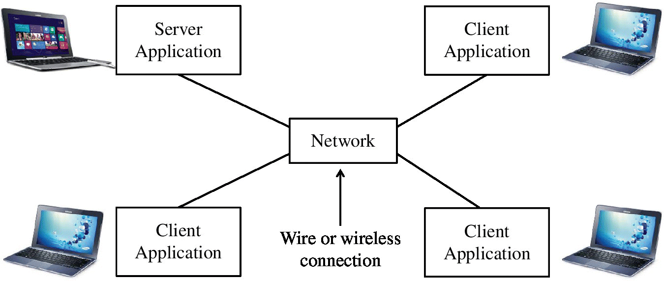
FIGURE 10.1 Client–server environment (star configuration)
Network Environment:
Each PC is connected to a hub that generally supports multiple PCs in a star configuration, as depicted in Figure 10.1. DEA results are transmitted through transmission control protocol/Internet protocol (TCP/IP). The TCP/IP allows interconnected PCs to be able to exchange information freely (e.g., DMUs to be evaluated, their inputs, desirable outputs and efficiency results) with each other as if these PCs were all directly connected together to each other. See Martin (1994) and Taniguchi (1998) that provided a detailed technical description on TCP/IP.
The architecture of TCP/IP has multiple layers. An application (upper) layer, in which the server prepares each data set, transforms the data set into digital signals, usually called “packets.” All the packets are shifted to a transport layer that provides a data delivery service. The application (bottom) layer exchanges messages through the transport layer that examines whether the data set is properly transformed into carrying packets. The TCP adds a header (i.e., information regarding what is being transmitted to the destination PC) to each packet at the transport layer.
These packets with TCP headers are shifted to the network layer where an IP header (i.e., the IP address of the source PC and that of the destination PC) is added to each carrying packet. Here, the IP header indicates a destination address that recognizes and specifies where each data set should be delivered in a computer network. The data set with TCP/IP headers is then shifted to the data link layer that controls all devices for network connection. The data link layer functions at the hub that transmits packets through the computer network. Thus, a hierarchical process of TCP/IP is established for network computing. See the research presented by Sueyoshi and Honma (2003) that visually discussed the hierarchical process of TCP/IP for network computing.
10.3 NETWORK COMPUTING FOR MULTI‐STAGE PARALLEL PROCESSES
10.3.1 Theoretical Preliminary
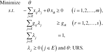
To describe the proposed network computing, this chapter starts with a description of the analytical structure, assuming that there are n DMUs. They are denoted by ![]() in this chapter. It is also assumed that no rank deficit occurs in the data domain for inputs and desirable outputs, as discussed in Chapter 2. Under these assumptions, DEA measures the level of efficiency on a specific DMU {k}, whose performance (Xk, Gk) is measured by the following input‐oriented model, or RM(v), which slightly reorganizes Model (4.4) as follows:
in this chapter. It is also assumed that no rank deficit occurs in the data domain for inputs and desirable outputs, as discussed in Chapter 2. Under these assumptions, DEA measures the level of efficiency on a specific DMU {k}, whose performance (Xk, Gk) is measured by the following input‐oriented model, or RM(v), which slightly reorganizes Model (4.4) as follows:

A difference between Models (4.4) and (10.1) is that the latter expresses a set of all DMUs by J for our descriptive convenience. As discussed in Chapter 4, the optimal θ* score of Model (10.1) indicates the level of operational efficiency (OEV) under variable RTS. In Model (10.1), ![]() and zero in all slacks indicates the state of full efficiency. In the other case, (e.g.,
and zero in all slacks indicates the state of full efficiency. In the other case, (e.g., ![]() and at least one positive slack) represents some level of inefficiency. For our descriptive convenience, Model (10.1) drops slacks from the objective function. As discussed in Chapters 4 and 5, there are seemingly efficient DMUs with
and at least one positive slack) represents some level of inefficiency. For our descriptive convenience, Model (10.1) drops slacks from the objective function. As discussed in Chapters 4 and 5, there are seemingly efficient DMUs with ![]() , but these DMUs belong to an inefficient DMU set (later referred to as IF and IF′ in this chapter) that contains a positive slack(s) on optimality. Chapter 4 considers that such a DMU is inefficient because of the existence of a positive slack(s).
, but these DMUs belong to an inefficient DMU set (later referred to as IF and IF′ in this chapter) that contains a positive slack(s) on optimality. Chapter 4 considers that such a DMU is inefficient because of the existence of a positive slack(s).
The development of network computing fully utilizes previous research results on the DEA special algorithm, first documented in Sueyoshi (1990, 1992). To briefly explain his algorithm, before extending it into the proposed network computing, this chapter starts with a description of the DMU classification, returning to Chapter 5. Here, it is important to note that Chapter 5 uses the DMU classification to describe differences between the Debreu–Farrell (radial) and the Pareto–Koopmans (non‐radial) measurements. Meanwhile, this chapter uses the DMU classification to describe an algorithm development on network computing.
According to the DMU classification discussed in Chapter 5, the whole set (J), representing all the DMUs, is first separated into the following two subsets Jd and Jn:
Equation (10.2) indicates that DMU j ' clearly outperforms DMU j where at least one inequality strictly satisfies the concept of “dominance.” A rationale for supporting Equation (10.2) is that the DMU j becomes clearly inefficient since the omission of such a clearly inefficient DMU group does not influence the whole assessment process of DEA. Thus, it is easily imagined that the inefficient DMU(s) should be eliminated at the beginning of DEA algorithm to reduce the whole computational burden. Of course, the performance of the clearly inefficient DMU(s) is evaluated, after all the other DMUs are evaluated, in the proposed algorithm.
Using Equation (10.2), the whole DMU set is separated into the following two DMU subsets:

Here, Jd is considered as a “dominated DMU set,” while Jn is the complement set for representing a “non‐dominated DMU set” (![]() ). As discussed in Chapter 5, the two DMU subsets are further classified as follows:
). As discussed in Chapter 5, the two DMU subsets are further classified as follows:
where

where the symbols (![]() and
and ![]() ) means “all” and “some,” respectively.
) means “all” and “some,” respectively.
Before describing the proposed network computing, the following conditions are necessary for the above DMU classification:
- First, all DMUs in E, E′ and IF′ have
 on optimality.
 - Second, differences among the three groups can be specified as follows: An occurrence of alternate optima (multiple solutions) may be found in E′ and IF′. In contrast, an optimal solution is unique for E.
- Third, the DMU(s) in IF′ has at least one positive slack on optimality, while the DMUs in E and E′ have no slack. Hence, a conclusive classification can be obtained by both searching for alternate optima and applying the second‐stage test using the additive model.
- Finally, the following computational processes are necessary for separation among E, E′ and IF′:
- Step 1: Solve Model (10.1) to obtain the optimal solution of DMU {k}. Then, the additive model is applied to DMU {k}. If the objective of the additive model is positive, then the DMU belongs to IF′. Meanwhile, if the objective is zero (so, all slacks are zero), the DMU belongs to either E or E′ and go to Step 2.
- Step 2: If
 is a non‐basic variable and its reduced cost is zero in the final tableau, then DMU {k} has alternate optima (so, multiple solution). In the case, it belongs to E′. Meanwhile, if
  is a basic variable, then the optimal solution of DMU {k} is unique and therefore, it belongs to E.
All the DMUs in IE and IF are “clearly inefficient” in terms of the dominance and non‐dominance relationship. So, the two groups consist of the dominated DMU set (Jd). Meanwhile, IE′ indicates a group of inefficient but non‐dominated DMUs. Alternate optima may occur on the three DMU groups (IF, IE and IE′).
Here, it is important to note that Sueyoshi and Chang (1989, p. 207) and Sueyoshi (1990, p. 250; 1992, p. 146) used the concept of dominance and non‐dominance in their algorithmic developments in order to identify the clearly inefficient (i.e., dominated) group of DMU(s) in the framework of radial and non‐radial models.
10.3.2 Computational Strategy for Network Computing
The development of the proposed network computing uses the following three major computation strategies:
- Strategy 1: When a data set becomes large (e.g., more than 1000 DMUs), the formulation can be expressed by the revised simplex tableau for Model (10.1) that consists of a long column (related to DMUs) and a relatively short row (related to inputs and desirable outputs). Therefore, it is easily imagined that the column reduction technique becomes an effective computation strategy4.
- Strategy 2: The DEA efficiency measurement of each DMU is determined by comparing its production achievement with an efficiency frontier (comprising efficient DMUs in
 ). Therefore, an effective DEA algorithm can identify the efficiency frontier in the early stage.
 - Strategy 3: The computational task is achieved in a distributed computing environment. The network computing reduces the computational load of each PC, and consequently reduces the total computation time to solve all DMUs. However, the use of network computing has a negative effect on the total computation time. That is, the total number of information exchanges (regarding optimal solution and DMUs to be solved) among PCs needs to be reduced because each information exchange needs a preparatory time to write an address to which information is transmitted. Many information exchanges among PCs may result in a considerable time loss.
10.3.3 Network Computing in Multi‐Stage Parallel Processes
Figure 10.2, obtained from Sueyoshi and Honma (2003), visually describes an algorithmic flow of the proposed network computing architecture. As depicted in the figure, the proposed computation is broken down into three stages. To explain the figure, we consider a computing environment in which a single server and z clients (c = 1,…, z) are connected to each other through the network, where c stands for the c‐th client PC.
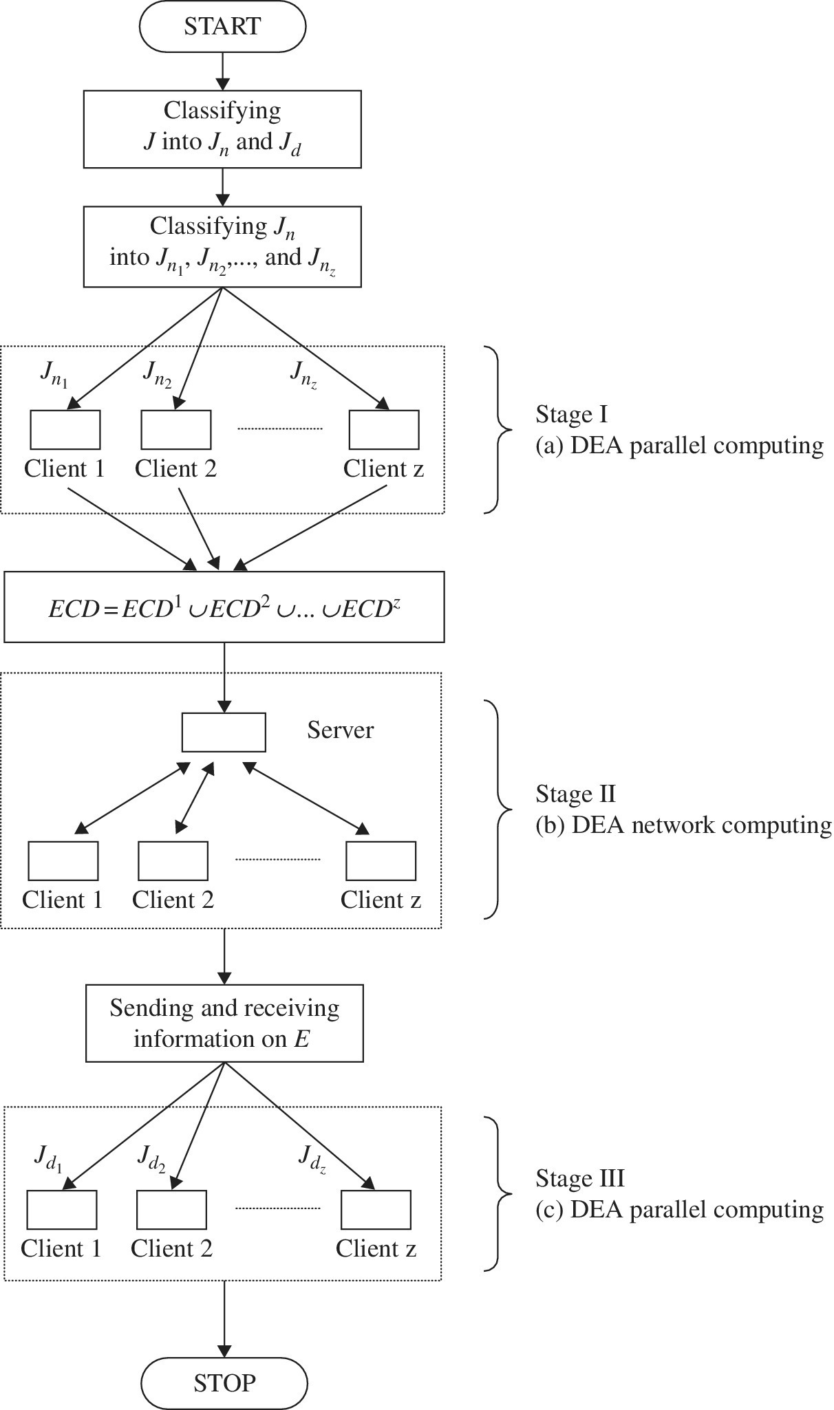
FIGURE 10.2 Computational strategy for network computing.
(a) Source: Sueyoshi and Honma (2003)
(b) This chapter reorganizes it for our description. ECD stands for efficiency candidates, which are a group of DMUs that may belong to  .
.
Preparatory:
Using Equation (10.2), a server classifies J (a whole DMU set) into Jn (a non‐dominated DMU set) and Jd (a dominated DMU set).
Stage I (Parallel computing for Jn):
A server randomly separates Jn into its subgroups (![]() ) and transmits information regarding which DMUs (
) and transmits information regarding which DMUs (![]() ) should be solved by the c‐th client. The number of DMUs in
) should be solved by the c‐th client. The number of DMUs in ![]() is referred to as a “block.” After evaluating all the DMUs in
is referred to as a “block.” After evaluating all the DMUs in ![]() , the c‐th client informs the server which DMUs become E‐candidates (ECD), implying that these DMUs may belong to
, the c‐th client informs the server which DMUs become E‐candidates (ECD), implying that these DMUs may belong to ![]() . The client solves only a subset of Jn. Therefore, the proposed algorithm is currently unable to make any decision regarding whether these E‐candidates are really efficient or inefficient because such are determined by the final evaluation. Here, the following subset (ECDc) is defined:
. The client solves only a subset of Jn. Therefore, the proposed algorithm is currently unable to make any decision regarding whether these E‐candidates are really efficient or inefficient because such are determined by the final evaluation. Here, the following subset (ECDc) is defined:
which indicates a set of the E‐candidates identified by the c‐th client. At the end of Stage I, the server can identify a whole set of E‐candidates as follows:
The ECD maintains the relationship such as ![]() . The CPU time of the c‐th client depends upon the number of DMUs in each subset (
. The CPU time of the c‐th client depends upon the number of DMUs in each subset (![]() ). The smaller the number becomes, the shorter the CPU time becomes at the c‐th client.
). The smaller the number becomes, the shorter the CPU time becomes at the c‐th client.
Stage II (Network computing for Jn):
The server sends all the clients information regarding which DMUs belong to ECD. Each client (e.g., the c‐th client) measures the efficiency measure of DMUs, belonging to ![]() , by using ECD. In this case, the simplex tableau contains the λ columns related to DMUs in ECD, not J (the whole DMU set). The columns related to inefficient DMUs are eliminated from the tableau. The set (E) is identified at the end of Stage II. Such DEA results are all transmitted to the server.
, by using ECD. In this case, the simplex tableau contains the λ columns related to DMUs in ECD, not J (the whole DMU set). The columns related to inefficient DMUs are eliminated from the tableau. The set (E) is identified at the end of Stage II. Such DEA results are all transmitted to the server.
Stage III (Parallel computing for Jd):
The sever sends all the clients information regarding which DMUs belong to E. The server separates Jd into its subgroups (![]() ) and then transmits information regarding which DMUs (
) and then transmits information regarding which DMUs (![]() ) should be solved by the c‐th client (c = 1,…, z). The client returns these DEA results to the server.
) should be solved by the c‐th client (c = 1,…, z). The client returns these DEA results to the server.
A computational flow of DEA network computing depicted in Figure 10.2 can be found in Barr and Durchholtz (1997). The approach is referred to as “hierarchical decomposition (HD)” that can be considered as three‐staged, parallel processes for partitioning a whole data set into blocks that are processed independently for DEA efficiency measurement. The premise is that if a DMU is inefficient within a block, then it is inefficient for any superset, including the whole DMU set. The inefficient DMUs are excluded from technology matrixes at the next stage. The process proceeds to aggregate blocks that are used for identification of efficient DMUs. A major difference between theirs (i.e., Barr and Durchholtz, 1997) and the proposed approach can be found in the fact that the latter is implemented in a client–server parallel system on modern computer technology.
10.3.3.1 Stage I (Parallel Computing for Jn )
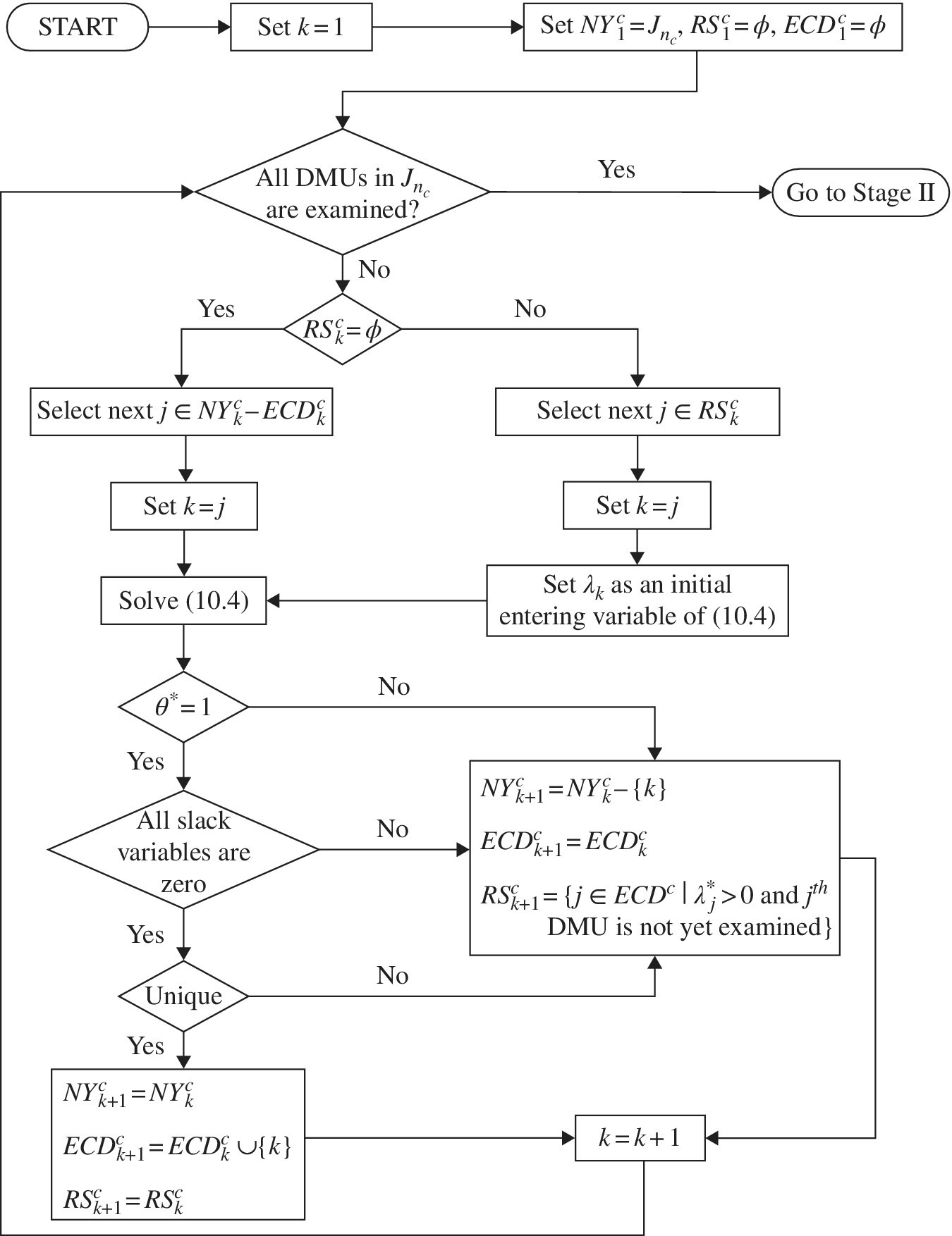
FIGURE 10.3 Stage I (parallel computing for Jn (a) Source: Sueyoshi and Honma (2003)). This chapter reorganizes it for our description. (b) NY: a group of DMUs which are “not yet” examined at the current stage.
Figure 10.3, obtained from Sueyoshi and Honma (2003), visually provides a detailed outline regarding Stage I. After receiving information on ![]() from the server, the c‐th client (c = 1,…, z) starts the following algorithmic process.
from the server, the c‐th client (c = 1,…, z) starts the following algorithmic process.
- Step 1: Set k = 1, where “k” is the number of steps and k = 1 implies the initial step. Note that the k‐th step has a one to one correspondence to the k‐th DMU to be currently evaluated by DEA. Thus, “k” indicates not only the step but also the order of DMU (J). Set
 ,
,  and
and  , where the symbol “φ” stands for an empty set. The superscript “c” indicates the c‐th client, as mentioned previously, and the subscript “1” stands for the first step.
 - Step k: Assuming that client c currently evaluates the k‐th DMU (so, the k‐th step), this study defines the following three subsets:

The first subset (
 ) is a subset of the E‐candidate set (ECDc) at the k‐th step of the c‐th client. The second subset (
 ) indicates
  plus a group of DMUs whose DEA efficiencies are “not yet” examined at the k‐th step of the c‐th client. The third set (
 ) indicates a reference set for
  . Before evaluating DMUs in
  , the proposed algorithm can predict that they belong to ECDc. Therefore, these DEA solutions are expressed by
  , all slacks are zero and they are unique.
Here, set k = j (![]() ), where
), where ![]() is a subset whose DMUs have not yet been examined by the c‐th client. Then, the OEV of the k‐th DMU is measured by the following model that is formulated by slightly modifying Model (10.1):
is a subset whose DMUs have not yet been examined by the c‐th client. Then, the OEV of the k‐th DMU is measured by the following model that is formulated by slightly modifying Model (10.1):

It is clear that ![]() gradually diminishes the size as the algorithm proceeds.
gradually diminishes the size as the algorithm proceeds. ![]() is observed at the last step of Stage I. The completion of the above algorithmic process indicates the end of Stage I.
is observed at the last step of Stage I. The completion of the above algorithmic process indicates the end of Stage I.
10.3.3.2 Stage II (Network Computing for Jn )
After receiving these DEA results from all the clients, Stage II starts the network computing in which both the server and the clients operate together through a network system in order to resume measuring the efficiency of all the DMUs in Jn. Figures 10.4 and 10.5, obtained from Sueyoshi and Honma (2003), visually describe the algorithmic process of the server and that of the c‐th client (c = 1,…, z), respectively.

FIGURE 10.4 Stage II (network computing for Jn (a) Source: Sueyoshi and Honma (2003)). This chapter reorganizes it for our description.

FIGURE 10.5 Network computing at the c‐th client.
(a) Source: Sueyoshi and Honma (2003)
This chapter reorganizes it for our description.
Server:
- Step 1: The server first sets
 ,
,  and
and  .
. - Step k:
- The server examines whether all the DMUs in Jn are evaluated.
- The server selects a client (e.g., the c‐th client) that is on standby, waiting for a job order from the server.
- After confirming whether the database of the c‐th client is updated, the server sends information on the k‐th DMU (
 ), along with ECDk, Ek and RSk, to the c‐th client.
 - The k‐th DMU is solved by the c‐th client. The server then receives information regarding DEA results on the DMU,
 ,
,  and
and  .
. - The database within the server is updated whenever DEA results are transmitted from the c‐th client.
The above computational process of the server is repeated until all the DMUs in ![]() are evaluated by DEA.
are evaluated by DEA.
The c‐th Client (c = 1, 2,…, z):
- Step 1: The c‐th client receives information on the k‐th DMU along with
 ,
,  and
and  from the server and updates its database.
 - Step k: The c‐th client measures the efficiency of the k‐th DMU (
 ) by(10.5)
The size of ECDk gradually diminishes as the algorithm proceeds and ![]() is observed at the last step of Stage II.
is observed at the last step of Stage II.
10.3.3.3 Stage III (Parallel Computing for Jd)
Figure 10.6 depicts the algorithmic process of Stage III. The server first separates Jd into z subsets such as ![]() The server transmits the c‐th client about information regarding which DMU {k} should be solved by the client.
The server transmits the c‐th client about information regarding which DMU {k} should be solved by the client.

FIGURE 10.6 Stage III (parallel computing for Jd at the c‐th client.
(a) Source: Sueyoshi and Honma (2003)
This chapter reorganizes it for our description.
The c‐th client measures the efficiency of DMU {k} (![]() ) by
) by
Since the revised simplex tableau has columns related to ![]() in Model (10.6), it is easily expected that the CPU time drastically reduces in particular when the number of inefficient DMUs is large because λj related to these DMUs are all omitted from Model (10.6). Moreover, z clients operate simultaneously under control of the server, so the total CPU time to solve all DMUs in Jd reduces as the number of clients increases. After each client solves Model (10.6), DEA results are transmitted to the server through the network. The completion of Stage III indicates the end of the whole computation of the proposed DEA network computing approach.
in Model (10.6), it is easily expected that the CPU time drastically reduces in particular when the number of inefficient DMUs is large because λj related to these DMUs are all omitted from Model (10.6). Moreover, z clients operate simultaneously under control of the server, so the total CPU time to solve all DMUs in Jd reduces as the number of clients increases. After each client solves Model (10.6), DEA results are transmitted to the server through the network. The completion of Stage III indicates the end of the whole computation of the proposed DEA network computing approach.
10.4 SIMULATION STUDY
A simulation study was applied to the proposed network computing, using artificially generated data sets. Four PCs were used for the simulation study. See Sueyoshi and Honma (2003) for the network configuration. Following the research efforts of Sueyoshi (1990, 1992) and Sueyoshi and Chang (1989), this chapter classified all DMUs into six different groups for the simulation study, which are specified as follows:
- First, efficient DMUs in E are designed to have the input vector X and the desirable output vector G whose components are generated by: x1 and x2 are selected from the uniform distribution of (3, 7),


- Second, efficient DMUs in Eʹ are generated as follows: two adjacent efficient DMUs, denoted by
 and
and  , are selected from the explicitly efficient DMU set (E) and then another type of efficient DMU in E′ is determined as a convex combination between (X,G) and (X′, G′) such as
  and
and  , where ω has values of (0, 1).
 - Third, inefficient DMUs in IE are generated as follows: the two adjacent efficient DMUs, or (X,G) and (X ′, G ′), are selected from E and then an input vector (
 ) of an inefficient DMU in IE is determined by
  , where ε is selected in a way that satisfies the following conditions:
  for i = 1, 2 and 3. Furthermore, three components of its desirable output vector are determined by
- Fourth, inefficient DMUs in IE ′ are generated as follows: two efficient DMUs, (X,G) and (X ′, G ′), are selected from E and then an input vector (
 ) of an inefficient DMU in IE ′ is determined by
  , where ε is selected in a way that satisfies the following conditions:
  , i = 1, 2 and 3. Furthermore, as specified for IE, the three components of the desirable output vector are determined by
- Fifth, after identifying an efficient DMU, denoted by (X,G), from E, we increase one component of the input vector to make an inefficient DMU in IF in either
 or
or  , where
  and
and  . Furthermore,
  is maintained for the desirable output vector.
 - Finally, two adjacent efficient DMUs, (X,G) and (X ′, G ′), are selected from E and then a DMU (X″, G ″) is determined by
 G″ = ωG + (1 − ω)G′. The input–output vector (
 ) of a DMU in IFʹ is determined by
  and
and  . Here,
  is maintained.
The above six DMU generations were repeated until we obtained the number of each DMU group needed for our simulation study. In this chapter, 3000 DMUs were generated for the first simulation and 10000 DMUs were generated for the second simulation.
The following additional two concerns are important in characterizing the proposed data generation process. One of the two concerns is that, as easily found in the structure of the proposed simulation, the number of input components is restricted to three and that of desirable output components are restricted to three (so, the number of these total dimensions is six) for generating the six different groups of DMUs. Of course, it is possible for us to generate these data sets by increasing the number of inputs and that of desirable outputs. However, in the case (more than three dimensions in an input vector or a desirable output vector), we cannot control the type of generated DMUs, as required by the proposed group classification. Consequently, it is difficult for us to examine how the percentage of efficient DMUs influences a speedup of the proposed network computing. Therefore, the proposed simulation study restricts the dimension of inputs plus desirable outputs to six. The other concern is that the proposed data generation started with the group (E) and then yielded the other groups of DMUs by extending E. To examine whether the data generation really produced such different groups, we reconfirmed all the generated DMUs by both searching for alternate optima and applying the second‐stage test by using the additive model.
The first simulation has examined how the CPU time of the proposed network computing approach is affected by a block size, a size of DMUs and a percentage of efficient DMUs. The structure of our simulation study can be summarized as follows:
- Number of DMUs: n = 1000, 1500, 2000, 2500 and 3000.
- Block size:
 = 50, 100, 150, 200, 250, 300, 350, 400, 450 and 500.
 - Percentage of efficient DMUs: pe = 10, 20, 30, 40 and 50%.
As indicated above, the structure of the first simulation study was a 5 × 10 × 5 factorial experiment in which each treatment had 200 replications, so totally 50000 (5 × 10 × 5 × 200) DEA evaluations were in the simulation study. Each replication produced a slightly different CPU time. Thus, we measured an average of these 200 replications on each treatment.
Table 10.1 compares CPU times of the proposed DEA network computing approach when the number of efficient DMUs ![]() is 20% of a whole DMU sample (J). The table lists CPU times used for the preparatory treatment for classifying J into Jn and Jd, Stage I (DEA parallel computing for Jn), Stage II (DEA network computing for Jn), and Stage III (DEA parallel computing for Jd), along with these total CPU times and average times (per DMU). Each average CPU time is listed within pointed parentheses (i.e., < >), next to each total CPU time. The unit of CPU time to be used for the proposed simulation study is the millisecond (MS), corresponding to 10–3 second. For example, see the two numbers 146817 and <48.94 > listed in the row label “Total” and a block size = 50 at the right‐hand side of Table 10.1. The two numbers indicate that 146817 MS, or 146.817 seconds, is necessary to complete a DEA efficiency measurement of 3000 DMUs on average. This implies that the proposed network computing approach needs, on average, 48.94 MS (=146 817/3000), or 0.04894 seconds to evaluate each DMU.
is 20% of a whole DMU sample (J). The table lists CPU times used for the preparatory treatment for classifying J into Jn and Jd, Stage I (DEA parallel computing for Jn), Stage II (DEA network computing for Jn), and Stage III (DEA parallel computing for Jd), along with these total CPU times and average times (per DMU). Each average CPU time is listed within pointed parentheses (i.e., < >), next to each total CPU time. The unit of CPU time to be used for the proposed simulation study is the millisecond (MS), corresponding to 10–3 second. For example, see the two numbers 146817 and <48.94 > listed in the row label “Total” and a block size = 50 at the right‐hand side of Table 10.1. The two numbers indicate that 146817 MS, or 146.817 seconds, is necessary to complete a DEA efficiency measurement of 3000 DMUs on average. This implies that the proposed network computing approach needs, on average, 48.94 MS (=146 817/3000), or 0.04894 seconds to evaluate each DMU.
TABLE 10.1 Comparison between CPU time and network computing
(a) Source: Sueyoshi and Honma (2003).
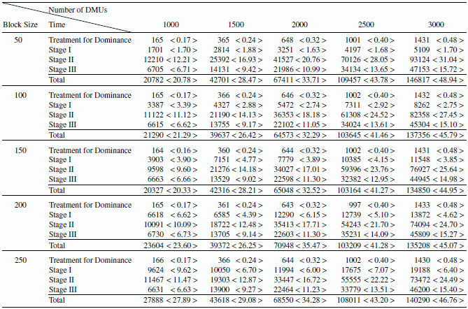
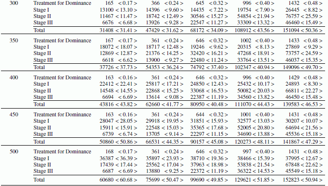
The finding of Table 10.1 is that the total CPU time is mutually affected by the number of DMUs. That is, the number of DMUs influences the total CPU time of the proposed network computing. CPU time is also influenced by a block size. This finding can be confirmed in the average CPU time, as well. For example, the average CPU time increases along with the number of DMUs, until the block size reaches 350. Similar CPU times are observed when the block size is 400. When the block size becomes more than 450, the average CPU time to measure 1000 DMUs is longer than that for 3000 DMUs. This result indicates that there may be an optimal combination between the block size and the number of DMUs in terms of minimizing the average CPU time.
Table 10.2 extends the simulation results of Table 10.1 by incorporating different percentages of efficient DMUs (pe = 10, 20, 30, 40 and 50%). The two numbers listed within curved, (), and square, [], brackets indicate the percentage of DMUs in E and E′, respectively. The finding of Table 10.2 is that the total CPU time reduces as the percentage of efficient DMUs decreases. The reduction of total CPU time occurs at any block size. This result is because the computational strategy incorporated into the network computing is effective when the number of efficient DMUs is small.
TABLE 10.2 Comparison between CPU time and network computing
(a) Source: Sueyoshi and Honma (2003).
| Efficient DMUs | Block Size | Number of DMUs | ||||
| 1000 | 1500 | 2000 | 2500 | 3000 | ||
| 10% (9%) [1%] | 50 | 14848 < 14.85 > | 30429 < 20.29 > | 47911 < 23.96 > | 67923 < 27.17 > | 96802 < 32.27 > |
| 100 | 15030 < 15.03 > | 28116 < 18.74 > | 45364 < 22.68 > | 64748 < 25.90 > | 87146 < 29.05 > | |
| 150 | 14556 < 14.56 > | 31381 < 20.92 > | 44313 < 22.16 > | 61994 < 24.80 > | 87549 < 29.18 > | |
| 200 | 16971 < 16.97 > | 28146 < 18.76 > | 49270 < 24.64 > | 65970 < 26.39 > | 84309 < 28.10 > | |
| 250 | 20302 < 20.30 > | 32542 < 21.69 > | 43480 < 21.74 > | 73151 < 29.26 > | 91180 < 30.39 > | |
| 300 | 24233 < 24.23 > | 36988 < 24.66 > | 47954 < 23.98 > | 61569 < 24.63 > | 98952 < 32.98 > | |
| 350 | 29503 < 29.50 > | 41510 < 27.67 > | 51680 < 25.84 > | 67282 < 26.91 > | 87083 < 29.03 > | |
| 400 | 35222 < 35.22 > | 45481 < 30.32 > | 59735 < 29.87 > | 73746 < 29.50 > | 88829 < 29.61 > | |
| 450 | 41475 < 41.48 > | 52826 < 35.22 > | 65888 < 32.94 > | 78328 < 31.33 > | 96826 < 32.28 > | |
| 500 | 48486 < 48.49 > | 60332 < 40.22 > | 73503 < 36.75 > | 84437 < 33.77 > | 103138 < 34.38 > | |
| 20% (18%) [2%] | 50 | 20782 < 20.78 > | 42701 < 28.47 > | 67411 < 33.71 > | 109457 < 43.78 > | 146817 < 48.94 > |
| 100 | 21290 < 21.29 > | 39637 < 26.42 > | 67573 < 33.79 > | 103645 < 41.46 > | 137356 < 45.79 > | |
| 150 | 20327 < 20.33 > | 42316 < 28.21 > | 65048 < 32.52 > | 103164 < 41.27 > | 134850 < 44.95 > | |
| 200 | 23604 < 23.60 > | 39372 < 26.25 > | 70948 < 35.47 > | 103209 < 41.28 > | 135208 < 45.07 > | |
| 250 | 27888 < 27.89 > | 43618 < 29.08 > | 68550 < 34.28 > | 108011 < 43.20 > | 140290 < 46.76 > | |
| 300 | 31408 < 31.41 > | 47429 < 31.62 > | 68172 < 34.09 > | 108912 < 43.56 > | 151094 < 50.36 > | |
| 350 | 37726 < 37.73 > | 54353 < 36.24 > | 74792 < 37.40 > | 102347 < 40.94 > | 149096 < 49.70 > | |
| 400 | 43816 < 43.82 > | 62660 < 41.77 > | 80950 < 40.48 > | 111070 < 44.43 > | 139583 < 46.53 > | |
| 450 | 50860 < 50.86 > | 66531 < 44.35 > | 90157 < 45.08 > | 120273 < 48.11 > | 141867 < 47.29 > | |
| 500 | 60680 < 60.68 > | 75699 < 50.47 > | 99690 < 49.85 > | 129621 < 51.85 > | 152823 < 50.94 > | |
| 30% (27%) [3%] | 50 | 25483 < 25.48 > | 52486 < 34.99 > | 90653 < 45.33 > | 128280 < 51.31 > | 191660 < 63.89 > |
| 100 | 27180 < 27.18 > | 51700 < 34.47 > | 87560 < 43.78 > | 121265 < 48.51 > | 186092 < 62.03 > | |
| 150 | 25951 < 25.95 > | 52756 < 35.17 > | 87069 < 43.53 > | 125601 < 50.24 > | 184184 < 61.39 > | |
| 200 | 29265 < 29.27 > | 53777 < 35.85 > | 94845 < 47.42 > | 124980 < 49.99 > | 190842 < 63.61 > | |
| 250 | 32758 < 32.76 > | 53532 < 35.69 > | 99627 < 49.81 > | 131770 < 52.71 > | 188523< 62.84 > | |
| 300 | 39562 < 39.56 > | 61934 < 41.29 > | 92144 < 46.07 > | 145174 < 58.07 > | 199530< 66.51 > | |
| 350 | 44296 < 44.30 > | 66396 < 44.26 > | 98644 < 49.32 > | 128710 < 51.48 > | 214637< 71.55 > | |
| 400 | 51410 < 51.41 > | 76415 < 50.94 > | 105775 < 52.89 > | 131985 < 52.79 > | 196409< 65.47 > | |
| 450 | 60300 < 60.30 > | 86044 < 57.36 > | 116584 < 58.29 > | 143271 < 57.31 > | 191095< 63.70 > | |
| 500 | 68605 < 68.61 > | 90255 < 60.17 > | 125068 < 62.53 > | 150331 < 60.13 > | 206448< 68.82 > | |
| 40% (36%) [4%] | 50 | 32781 < 32.78 > | 63527 < 42.35 > | 112737 < 56.37 > | 161993 < 64.80 > | 239979< 79.99 > |
| 100 | 33019 < 33.02 > | 63632 < 42.42 > | 114637 < 57.32 > | 162870 < 65.15 > | 235540< 78.51 > | |
| 150 | 33792 < 33.79 > | 69645 < 46.43 > | 116347 < 58.17 > | 158784 < 63.51 > | 242999< 81.00 > | |
| 200 | 36272 < 36.27 > | 76660 < 51.11 > | 115289 < 57.64 > | 162134 < 64.85 > | 243524< 81.17 > | |
| 250 | 40143 < 40.14 > | 67753 < 45.17 > | 125584 < 62.79 > | 172203 < 68.88 > | 233544< 77.85 > | |
| 300 | 46545 < 46.55 > | 76330 < 50.89 > | 118810 < 59.41 > | 186018 < 74.41 > | 248437< 82.81 > | |
| 350 | 52378 < 52.38 > | 81988 < 54.66 > | 119761 < 59.88 > | 183770 < 73.51 > | 263458< 87.82 > | |
| 400 | 59099 < 59.10 > | 92479 < 61.65 > | 129997 < 65.00 > | 174947 < 69.98 > | 271361< 90.45 > | |
| 450 | 67397 < 67.40 > | 100384 < 66.92 > | 134476 < 67.24 > | 184471 < 73.79 > | 253894< 84.63 > | |
| 500 | 77365 < 77.37 > | 111245 < 74.16 > | 145868 < 72.93 > | 191445 < 76.58 > | 248793< 82.93 > | |
| 50% (45%) [5%] | 50 | 38501 < 38.50 > | 85288 < 56.86 > | 140295 < 70.15 > | 209541 < 83.82 > | 300725 < 100.24 > |
| 100 | 39884 < 39.88 > | 85568 < 57.05 > | 136631 < 68.32 > | 205000 < 82.00 > | 304783 < 101.59 > | |
| 150 | 41898 < 41.90 > | 86034 < 57.36 > | 141340 < 70.67 > | 202782 < 81.11 > | 302465 < 100.82 > | |
| 200 | 41677 < 41.68 > | 91336 < 60.89 > | 142500 < 71.25 > | 199022 < 79.61 > | 304713 < 101.57 > | |
| 250 | 46185 < 46.19 > | 87041 < 58.03 > | 152233 < 76.12 > | 211760 < 84.70 > | 306125 < 102.04 > | |
| 300 | 53072 < 53.07 > | 89509 < 59.67 > | 153432 < 76.72 > | 220517 < 88.21 > | 312769 < 104.26 > | |
| 350 | 59667 < 59.67 > | 98272 < 65.51 > | 147141 < 73.57 > | 234573 < 93.83 > | 330784 < 110.26 > | |
| 400 | 64717 < 64.72 > | 107035 < 71.36 > | 155468 < 77.73 > | 216236 < 86.49 > | 347891 < 115.96 > | |
| 450 | 73847 < 73.85 > | 113568 < 75.71 > | 168643 < 84.32 > | 216536 < 86.61 > | 336072 < 112.02 > | |
| 500 | 83768 < 83.77 > | 126302 < 84.20 > | 173310 < 86.66 > | 227507 < 91.00 > | 323348 < 107.78 > | |
Next, we examined how the number of PCs (clients) influences the total CPU time. The structure of this simulation study may be summarized as follows:
- Number of DMUs: n = 1000, 1500, 2000, 2500, 3000, 5000, 7500, 10000
- Number of PCs: z = 1, 2, 3 and 4
- Percentage of efficient DMUs: pe = 10, 20, 30, 40 and 50%
Thus, the second simulation had the structure of an 8 × 4 × 5 factorial experiment in which each treatment had 200 replications, so that a total of 32000 (8 × 4 × 5 × 200) DEA evaluations were conducted for the whole simulation study.
The computational results of the second simulation study are documented in both Tables 10.3 and 10.4. Table 10.3 compares the CPU times of the proposed DEA network for computing when the block size is 50 and the percentage of efficient DMUs (![]() ) is 20%. Table 10.3 indicates that the total and average CPU times have an increasing trend, corresponding to the number of DMUs. However, the rate of the increasing trend diminishes as the number of PCs increases. For example, the average CPU time is 39.00 MS when two PCs are used for network computing and 1000 DMUs are evaluated by DEA. The corresponding average CPU time becomes 20.78 MS when the number of PCs increases from two to four. Such a change in the number of PCs reduces the average CPU time by 47% [= (1 – 20.78)/39.00]. The decrease in the total and average CPU times can be found in the DEA evaluation of all the numbers of DMUs listed in Table 10.3.
) is 20%. Table 10.3 indicates that the total and average CPU times have an increasing trend, corresponding to the number of DMUs. However, the rate of the increasing trend diminishes as the number of PCs increases. For example, the average CPU time is 39.00 MS when two PCs are used for network computing and 1000 DMUs are evaluated by DEA. The corresponding average CPU time becomes 20.78 MS when the number of PCs increases from two to four. Such a change in the number of PCs reduces the average CPU time by 47% [= (1 – 20.78)/39.00]. The decrease in the total and average CPU times can be found in the DEA evaluation of all the numbers of DMUs listed in Table 10.3.
TABLE 10.3 Comparison between CPU time and network computing
(a) Source: Sueyoshi and Honma (2003). (b) It was impossible to measure a CPU time of DEA problems that contained more than 2000 DMUs by a single PC.
| # of PCs | Treatment | Number of DMUs | |||||||
| 1000 | 1500 | 2000 | 2500 | 3000 | 5000 | 7500 | 10000 | ||
| 1 | Dominance Computation | 1731 | 2592 | 4506 | Unable to measure | ||||
| 65306 | 147293 | 253747 | |||||||
| TotalAverage (per DMU) | 67037 | 149885 | 258253 | ||||||
| 67.04 | 99.92 | 129.13 | |||||||
| 2 | Dominance | 160 | 360 | 661 | 991 | 1502 | 3425 | 7401 | 13049 |
| Stage I | 5428 | 7731 | 10315 | 12428 | 16644 | 14821 | 17545 | 27579 | |
| Stage II | 20068 | 37645 | 70821 | 110298 | 163505 | 425342 | 731999 | 1652507 | |
| Stage III | 13340 | 24154 | 29938 | 68899 | 78213 | 279081 | 520041 | 127200 | |
| TotalAverage (per DMU) | 38996 | 69890 | 111735 | 192616 | 259864 | 722669 | 1276986 | 1820335 | |
| 39.00 | 46.59 | 55.87 | 77.05 | 86.62 | 144.53 | 170.26 | 182.03 | ||
| 3 | Dominance | 161 | 360 | 661 | 992 | 1502 | 3425 | 7401 | 12859 |
| Stage I | 3615 | 5288 | 7031 | 9223 | 11046 | 9915 | 12037 | 18707 | |
| Stage II | 13679 | 26168 | 46787 | 76650 | 110539 | 284999 | 534725 | 1102184 | |
| Stage III | 9504 | 17054 | 27770 | 47068 | 53106 | 188431 | 358580 | 874748 | |
| TotalAverage (per DMU) | 26959 | 48870 | 82249 | 133933 | 176193 | 486770 | 912743 | 2008498 | |
| 26.96 | 32.58 | 41.12 | 53.57 | 58.73 | 97.35 | 121.70 | 200.85 | ||
| 4 | Dominance | 165 | 365 | 648 | 1001 | 1431 | 3415 | 7411 | 12978 |
| Stage I | 1701 | 2814 | 3251 | 4197 | 5109 | 7792 | 9704 | 14481 | |
| Stage II | 12210 | 25392 | 41527 | 70126 | 93124 | 217572 | 437154 | 821922 | |
| Stage III | 6705 | 14131 | 21986 | 34134 | 47153 | 134143 | 249633 | 609286 | |
| TotalAverage (per DMU) | 20781 | 42702 | 67412 | 109458 | 146817 | 362922 | 703902 | 1458667 | |
| 20.78 | 28.47 | 33.71 | 43.78 | 48.94 | 72.58 | 93.85 | 145.87 | ||
TABLE 10.4 Comparison between CPU time and network computing
(a) Source: Sueyoshi and Honma (2003).
| # of PCs | Efficient DMUs | Number of DMUs | |||||||
| 1000 | 1500 | 2000 | 2500 | 3000 | 5000 | 7500 | 10000 | ||
| 1 | 10%(9%)[1%] | 52981 < 52.98 > | 111793 < 74.53 > | 173579 < 86.79 > | Unable to measure | ||||
| 20%(18%)[2%] | 67037 < 67.04 > | 149885 < 99.92 > | 258253 < 129.13 > | ||||||
| 30%(27%)[3%] | 86165 < 86.17 > | 190187 < 126.79 > | 345827 < 172.91 > | ||||||
| 40%(36%)[4%] | 113827 < 113.83 > | 241089 < 160.73 > | 403125 < 201.56 > | ||||||
| 50%(45%)[5%] | 124577 < 124.58 > | 279396 < 186.26 > | 496588 < 248.29 > | ||||||
| 2 | 10%(9%)[1%] | 25477 < 25.48 > | 51494 < 34.33 > | 82378 < 41.19 > | 120704 < 48.28 > | 170625 < 56.88 > | 503604 < 100.72 > | 836894 < 111.59 > | 1723428 < 172.34 > |
| 20%(18%)[2%] | 38996 < 39.00 > | 69890 < 46.59 > | 111735 < 55.87 > | 192616 < 77.05 > | 259864 < 86.62 > | 722669 < 144.53 > | 1276986 < 170.26 > | 2965835 < 296.58 > | |
| 30%(27%)[3%] | 49712 < 49.71 > | 91792 < 61.19 > | 179208 < 89.60 > | 248467 < 99.39 > | 330075 < 110.03 > | 977576 < 195.52 > | 1962943 < 261.73 > | 3775659 < 377.57 > | |
| 40%(36%)[4%] | 59175 < 59.18 > | 121164 < 80.78 > | 243560 < 121.78 > | 348752 < 139.50 > | 514349 < 171.45 > | 1175961 < 235.19 > | 2418247 < 322.43 > | 5016553 < 501.66 > | |
| 50%(45%)[5%] | 78283 < 78.28 > | 180830 < 120.55 > | 274695 < 137.35 > | 392314 < 156.93 > | 612591 < 204.20 > | 1633409 < 326.68 > | 3120748 < 416.10 > | 6201888 < 620.19 > | |
| 3 | 10%(9%)[1%] | 17816 < 17.82 > | 38005 < 25.34 > | 56241 < 28.12 > | 84942 < 33.98 > | 113693 < 37.90 > | 343554 < 68.71 > | 599482 < 79.93 > | 1150714 < 115.07 > |
| 20%(18%)[2%] | 26959 < 26.96 > | 48870 < 32.58 > | 82249 < 41.12 > | 133933 < 53.57 > | 176193 < 58.73 > | 486770 < 97.35 > | 912743 < 121.70 > | 2008498 < 200.85 > | |
| 30%(27%)[3%] | 36592 < 36.59 > | 62339 < 41.56 > | 120724 < 60.36 > | 167281 < 66.91 > | 220928 < 73.64 > | 652588 < 130.52 > | 1284968 < 171.33 > | 2261692 < 226.17 > | |
| 40%(36%)[4%] | 42260 < 42.26 > | 84030 < 56.02 > | 163195 < 81.60 > | 233926 < 93.57 > | 345557 < 115.19 > | 786301 < 157.26 > | 1617486 < 215.66 > | 3202955 < 320.30 > | |
| 50%(45%)[5%] | 53617 < 53.62 > | 132356 < 88.24 > | 183553 < 91.78 > | 269397 < 107.76 > | 407455 < 135.82 > | 1081005 < 216.20 > | 2073321 < 276.44 > | 4171137 < 417.11 > | |
| 4 | 10%(9%)[1%] | 14848 < 14.85 > | 30429 < 20.29 > | 47911 < 23.96 > | 67923 < 27.17 > | 96802 < 32.27 > | 271420 < 54.28 > | 473561 < 63.14 > | 898112 < 89.81 > |
| 20%(18%)[2%] | 20782 < 20.78 > | 42701 < 28.47 > | 67411 < 33.71 > | 109457 < 43.78 > | 146817 < 48.94 > | 362922 < 72.58 > | 703902 < 93.85 > | 1458667 < 145.87 > | |
| 30%(27%)[3%] | 25483 < 25.48 > | 52486 < 34.99 > | 90653 < 45.33 > | 128280 < 51.31 > | 191660 < 63.89 > | 484437 < 96.89 > | 1033556 < 137.81 > | 1936935 < 193.69 > | |
| 40%(36%)[4%] | 32781 < 32.78 > | 63527 < 42.35 > | 112737 < 56.37 > | 161993 < 64.80 > | 239979 < 79.99 > | 602186 < 120.44 > | 1225402 < 163.39 > | 2509158 < 250.92 > | |
| 50%(45%)[5%] | 38501 < 38.50 > | 85288 < 56.86 > | 140295 < 70.15 > | 209541 < 83.82 > | 300725 < 100.24 > | 824235 < 164.85 > | 1470154 < 196.02 > | 3110954 < 311.10 > | |
Based upon this result, we may predict an extended case in which the total CPU time, incorporating more than four PCs in the network, becomes less than that of the four PCs. However, the reduction rate is less than that which occurs when the number of PCs is changed from three to four. Thus, it is expected that there is an optimal number of PCs for the proposed network computing that is determined by a combination of the decrease in CPU time within the PCs and the increase in network communication time between them. Network computing may not lessen the total CPU time if the number of PCs is beyond the optimal number.
Each PC in network computing fully utilizes the proposed algorithmic strategy, but it has a limitation on computational improvement. For example, a single PC operation to solve more than 2500 DMUs needs a long computational time (for example, more than 10 hours). So, our simulation terminates the CPU time measurement of single PC operation for more than 2000 DMUs. The proposed network implementation can easily overcome such a limitation in terms of solving large‐scale DEA problems by fully utilizing network technology (e.g., a client–server function) to synchronize multiple PCs.
Table 10.4 generalizes the simulation results of Table 10.3 by incorporating different percentages (pe = 10, 20, 30, 40 and 50%) of efficient DMUs. As summarized in Table 10.4, the average CPU time shows an increasing trend matching the number of DMUs. The increasing rate is affected by not only the number of PCs but also the percentage of efficient DMUs. For example, the combination between z = 2 and pe = 50% produces the highest (or the most time‐consuming) average CPU time among the six combinations. The second highest is the combination between z = 2 and pe = 30%. However, the third highest time‐consuming combination is the one for z = 4 and pe = 50%. This is a surprising result. Thus, the average CPU time and related increasing rate are affected by both the number of PCs and the percentage of efficient DMUs.
10.5 SUMMARY
To deal with large DEA problems, this chapter proposed the architecture of network computing that was designed to synchronize multiple PCs in a client–server parallel implementation. Each PC in the network managed its own memory in order to evaluate the performance of DMUs on Microsoft Excel. An important feature of this network computing was that it was computationally structured in multi‐stage parallel processes: (a) preparatory treatment for classifying all the DMUs into two subsets (Jn: a non‐dominated DMU set; Jd: a dominated DMU set), (b) Stage I (DEA parallel computing for Jn), (c) Stage II (DEA network computing for Jn) and (d) Stage III (DEA parallel computing for Jd). Thus, network computing, which was designed to fully utilize both modern network technology and special algorithmic strategies, enhanced the algorithmic efficiency to solve various large problems. The performance of the proposed network computing was examined in a large simulation study that compared the CPU times by controlling the number of DMUs, the percentage of efficient DMUs, the size of block and the number of PCs.
Here, it is necessary to mention that the computational results were listed in a previous research effort (Sueyoshi and Honma, 2003). It is indeed true that their simulation results were based upon an old type of PC configuration that might be obsolete under modern PC technology. However, the proposed architecture for network computing is still useful and computationally efficient in dealing with a large data set on DEA even now.
Paying attention to modern computer technology, this chapter needs to discuss four problems. First, this chapter has discussed only local area network computing. The computational feature needs to be extended into wide area network computing and further, “cloud computing” and a super computer, which make it possible that we can simultaneously operate computing devices all over the world. Parallel processing, using networks of PCs, is the current form of distributed computing and it is a realistic computing environment for DEA applications. Hence, such a physical network expansion is an important future research task. Second, as explored in Gonzalez–Lima et al. (1996), it is possible for us to use a modern algorithm (e.g., the interior point method) to solve various DEA performance assessments. Third, the proposed approach did not explore the analytical relationship between problem size (i.e., the number of DMUs) and computation time. How large is the best block size? No reply was discussed in this chapter. Finally, the proposed network computing approach can be useful in various DEA applications. The proposed approach does not document such empirical results, in particular DEA environmental assessment. That will be an important research task.