
12
Real-Time, Task-Based Scheduling
CONTENTS
12.1 Fixed and Variable Task Priority
12.1.2 Variable Priority in General Purpose Operating Systems
12.2.1 Proof of Rate Monotonic Optimality
The previous chapter has introduced the basic model and terminology for real-time scheduling. The same notation will be used in this chapter as well as in the following ones, and therefore, it is briefly recalled here. A periodic real-time process is called a task and denoted by τi. A task models a periodic activity: at the j-th occurrence of the period Ti a job τi,j for a given task τi is released. The job is also called an instance of the task τi. The relative deadline Di for a task τi represents the maximum time allowed between the release of any job τi,j and its termination, and, therefore, the absolute deadline di,j for the job τi,j is equal to its release time plus the relative deadline. The worst-case execution time of task Ti represents the upper limit of the processor time required for the computation of any job for that task, while Ri indicates the worst-case response time of task Ti, that is, the maximum elapsed time between the release of any job for this task and its termination. The worst-case execution time (WCET) Ci is the time required to complete any job of the task τi without any interference from other activities. Finally, fi,j is the actual absolute response time (i.e., the time of its termination) for job τi,j of task τi.
While in the cyclic executive scheduling policy all jobs were executed in a predefined order, in this chapter we shall analyze a different situation where tasks correspond to processes or threads and are therefore scheduled by the operating system based on their current priority. Observe that, in the cyclic executive model, there is no need for a scheduler at all: the jobs are represented by routines that are invoked in a predefined order by a single program. Here we shall refer to a situation, which is more familiar to those who have read the first part of this book, where the operating system handles the concurrent execution of different units of execution. In the following, we shall indicate such units as tasks, being the distinction between processes and threads not relevant in this context. Depending on the practical requirements, tasks will be implemented either by processes or threads, and the results of the scheduling analysis are valid in both cases.
Many of the results presented in this chapter and in the following ones are due to the seminal work of Liu and Layland [60], published in 1973. Several proofs given in the original paper have later been refined and put in a more intuitive form by Buttazzo [19]. Interested readers are also referred to Reference [78] for more information about the evolution of real-time scheduling theory from a historical perspective. Moreover, References [19, 61] discuss real-time scheduling in much more formal terms than can be afforded here, and they will surely be of interest to readers with a stronger mathematical background.
12.1 Fixed and Variable Task Priority
We have seen in Chapter 3 that the priority associated with tasks is an indication of their “importance.” Important tasks need to be executed first, and therefore, the scheduler, that is, the component of the operating system that supervises the assignment of the processors to tasks, selects the task with the highest priority among those that are currently ready (i.e., which are not in wait state, due, for example, to a pending I/O operation). Therefore, the policy that is adopted to assign priorities to tasks determines the behavior of the scheduling. In the following, we shall analyze different policies for assigning priorities to tasks and their impact in obtaining the desired real-time behavior, making sure that every job terminates within its assigned deadline.
12.1.1 Preemption
Before discussing about priority assignment policies, we need to consider an important fact: what happens if, during the execution of a task at a given priority, another task with higher priority becomes ready? Most modern operating systems in this case reclaim the processor from the executing task and assign it to the task with higher priority by means of a context switch. This policy is called preemption, and it ensures that the most important task able to utilize the processor is always executing. Older operating systems, such as MS-DOS or the Mac OS versions prior to 10, did not support preemption, and therefore a task that took possession of the processor could not be forced to release it, unless it performed an I/O operation or invoked a system call. Preemption presents several advantages, such as making the system more reactive and preventing rogue tasks from monopolizing the processor. The other side of the coin is that preemption is responsible for most race conditions due to the possibly unforeseen interleaved execution of higher-priority tasks.
Since in a preemptive policy the scheduler must ensure that the task currently in execution is always at the highest priority among those that are ready, it is important to understand when a context switch is possibly required, that is, when a new higher priority task may request the processor. Let us assume first that the priorities assigned to tasks are fixed: a new task may reclaim the processor only when it becomes ready, and this may happen only when a pending I/O operation for that task terminates or a system call (e.g., waiting for a semaphore) is concluded. In all cases, such a change in the task scenario is carried out by the operating system, which can therefore effectively check current task priorities and ensure that the current task is always that with the highest priority among the ready ones. This fact holds also if we relax the fixed-priority assumption: the change in task priority would be in any case carried out by the operating system, which again is aware of any possible change in the priority distribution among ready tasks.
Within the preemptive organization, differences may arise in the management of multiple ready tasks with the same highest priority. In the following discussion, we shall assume that all the tasks have a different priority level, but such a situation represents somehow an abstraction, the number of available priority levels being limited in practice. We have already seen that POSIX threads allow two different management of multiple tasks at the same highest priority tasks:
The First In First Out (FIFO) management, where the task that acquires the processor will execute until it terminates or enters in wait state due to an I/O operation or a synchronization primitive, or a higher priority task becomes ready.
The Round Robin (RR) management where after some amount of time (often called time slice) the running task is preempted by the scheduler even if no I/O operation is performed and no higher-priority task is ready to let another task at the same priority gain processor usage.
12.1.2 Variable Priority in General Purpose Operating Systems
Scheduling analysis refers to two broad categories in task priority assignment to tasks: Fixed Priority and Variable Priority. As the name suggests, in fixed priority scheduling, the priority assigned to tasks never changes during system execution. Conversely, in the variable-priority policy, the priority of tasks is dynamically changed during execution to improve system responsiveness or other parameters. Before comparing the two approaches, it is worth briefly describing what happens in general-purpose operating systems such as Linux and Windows. Such systems are intended for a variety of different applications, but interaction with a human user is a major use case and, in this case, the perceived responsiveness of the system is an important factor. When interacting with a computer via a user interface, in fact, getting a quick response to user events such as the click of the mouse is preferable over other performance aspects such as overall throughput in computation. For this reason, a task that spends most of its time doing I/O operations, including the response to user interface events, is considered more important than a task making intensive computation. Moreover, when the processor is assigned to a task making lengthy computation, if preemption were not supported by the scheduler, the user would experience delays in interaction due to the fact that the current task would not get a chance to release the processor if performing only computation and not starting any I/O. For these reasons, the scheduler in a general purpose operating system will assign a higher priority to I/O intensive tasks and will avoid that a computing-intensive task monopolize the processor, thus blocking interaction for an excessively long period. To achieve this, it is necessary to provide an answer to the following questions:
How to discriminate between I/O-intensive and computing-intensive tasks?
How to preempt the processor from a computing-intensive task that is not willing to relinquish it?
How to ensure enough fairness to avoid that a ready task is postponed forever or for a period of time that is too long?
The above problems are solved by the following mechanism for dynamic priority assignment, called timesharing, which relies on a clock device that periodically interrupts the processor and gives a chance to the operating system to get control, rearrange task priorities and possibly operate a context switch because a task with a higher priority than the current one is now available. Interestingly enough, many dynamic priority assignment schemes in use today still bear a strong resemblance to the scheduling algorithm designed by Corbató [21] back in 1962 for one of the first experimental timesharing systems.
A time slice (also called quantum) is assigned to every task when it acquires the processor, and at every clock period (called tick), the operating system decreases the quantum value of the running task in case no other task with a higher priority becomes ready. When the quantum reaches 0, and there is at least another task with equal or higher priority, the current task is preempted. In addition to the quantum mechanism, a variable is maintained by the operating system for each task: whenever the task is awakened, this variable is incremented; whenever the task is preempted or its quantum expires, the variable is decremented.
The actual value of the variable is used to compute a “priority bonus” that rewards I/O-intensive tasks that very seldom experience quantum expiration and preemption (an I/O-intensive task is likely to utilize the processor for a very short period of time before issuing a new I/O and entering in wait state), and which penalizes computing-intensive tasks that periodically experience quantum expiration and are preempted.
In this way, discrimination between I/O and computing-intensive tasks is carried out by the actual value of the associated task variable, the quantum expiration mechanism ensures that the processor is eventually preempted from tasks that would otherwise block the system for too long, and the dynamic priority mechanism lowers the priority of computing-intensive tasks that would otherwise block lower priority tasks waiting for the processor. Observe that I/O-intensive tasks will hardly cause any task starvation since typically they require the processor for very short periods of time.
Timesharing is an effective policy for interactive systems but cannot be considered in real-time applications because it is not possible to predict in advance the maximum response time for a given task since this depends on the behavior of the other tasks in the systems, affecting the priority of the task and therefore its response time. For this reason, real-time systems normally assign fixed priorities to tasks, and even general-purpose operating systems supporting timesharing reserve a range of higher priorities to be statically assigned to real-time tasks. These tasks will have a priority that is always higher than the priority of timesharing tasks and are therefore guaranteed to get the processor as soon as they become ready, provided no higher-priority real-time task is currently ready. The next section will present and analyze a widely adopted policy called Rate Monotonic in fixed-priority assignment. The reader may, at this point, wonder whether dynamic priority assignment can be of any help in real-time applications. The next section shows that this is the case and presents a dynamic priority assignment policy, called Earliest Deadline First, which not only ensures real-time behavior in a system of periodic tasks, but represents the “best” scheduling policy ever attainable for a given set of periodic tasks under certain conditions as described in the following pages.
12.2 Rate Monotonic
Rate monotonic is a policy for fixed-priority assignment in periodic tasks, which assigns a priority that is inversely proportional to the task period: the shorter the task period, the higher its priority. Consider, for example, the three tasks listed in Table 12.1: task τ1, which has the smallest period, will have the highest priority, followed by tasks τ3 and τ2, in that order.
Observe hat the priority assignment takes into account only the task period, and not the effective computation time. Priorities are often expressed by integers, but there is no general agreement on whether higher values represent higher priorities or the other way round. In most cases, lower numbers indicate higher priorities, but in any case, this is only an implementation issue and does not affect the following discussion.
TABLE 12.1
An example of Rate Monotonic priority assignment
| Task | Period | Computation Time | Priority |
| τ1 | 20 | 7 | High |
| τ2 | 50 | 13 | Low |
| τ3 | 25 | 6 | Medium |
In order to better understand how a scheduler (the rate monotonic scheduler in this case) works, and to draw some conclusions about its characteristics, we can simulate the behavior of the scheduler and build the corresponding scheduling diagram. To be meaningful, the simulation must be carried out for an amount of time that is “long enough” to cover all possible phase relations among the tasks. As for the cyclic executive, the right amount of time is the Least Common Multiple (LCM) of the task periods. After such period, if no overflow occurs (i.e., the scheduling does not fail), the same sequence will repeat, and therefore, no further information is obtained when simulation of the system behavior is performed for a longer period of time. Since we do not have any additional information about the tasks, we also assume that all tasks are simultaneously released at t = 0. We shall see shortly that this assumption is the most pessimistic one when considering the scheduling assignment, and therefore, if we prove that a given task priority assignment can be used for a system, that it will be feasible regardless of the actual initial release time (often called phase) of task jobs. A sample schedule is shown in Figure 12.1.
The periods of the three tasks are 20 ms, 25 ms and 50 ms, respectively, and therefore the period to be considered in simulation is 100ms, that is the Least Common Multiplier of 20, 25 and 50. At t = 0, all tasks are ready: the first one to be executed is τ1 then, at its completion, τ3. At t = 13 ms, τ2finally starts but, at t = 20 ms, τ1 is released again. Hence, τ2 is preempted in favor of τ1. While τ1 is executing, τ3 is released, but this does not lead to a preemption: τ3 is executed after τ1 has finished. Finally, τ2 is resumed and then completed at t = 39 ms. At t = 40 ms, after 1 ms of idling, task τ1 is released. Since it is the only ready task, it is executed immediately, and completes at t = 47 ms. At t = 50ms, both τ3 and τ2 become ready simultaneously. τ3 is run first, then τ2 starts and runs for 4 ms. However, at t = 60 ms, τ1 is released again. As before, this leads to the preemption of τ2 and τ1 runs to completion. Then, τ2 is resumed and runs for 8 ms, until τ3 is released. τ2 is preempted again to run τ3. The latter runs for 5 ms but at, t = 80 ms, τ1 is released for the fifth time. τ3 is preempted, too, to run τ1. After the completion of τ1,both τ3 and τ2 are ready. τ3 runs for 1 ms, then completes. Finally, τ2 runs and completes its execution cycle by consuming 1 ms of CPU time. After that, the system stays idle until t = 100 ms, where the whole cycle starts again.
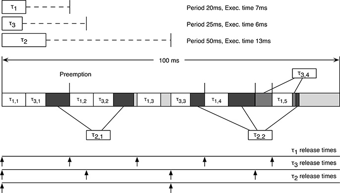
FIGURE 12.1
Scheduling sequence for tasks τ1, τ2, and τ3.
Intuitively Rate Monotonic makes sense: tasks with shorter period are expected to be executed before others because they have less time available. Conversely, a task with a long period can afford waiting for other more urgent tasks and finish its execution in time all the same. However intuition does not represent a mathematical proof, and we shall prove that Rate Monotonic is really the best scheduling policy among all the fixed priority scheduling policies. In other words, if every task job finishes execution within its deadline under any given fixed priority assignment policy, then the same system is feasible under Rate Monotonic priority assignment. The formal proof, which may be skipped by the less mathematically inclined reader, is given below.
12.2.1 Proof of Rate Monotonic Optimality
Proving the optimality of Rate Monotonic consists in showing that if a given set of periodic tasks with fixed priorities is schedulable in any way, then it will be schedulable using the Rate Monotonic policy. The proof will be carried out under the following assumptions:
Every task τi is periodic with period Ti.
The relative deadline Di for every task τi is equal to its period Ti.
Tasks are scheduled preemptively and according to their priority.
There is only one processor.
We shall prove this in two steps. First we shall introduce the concept of “critical instant,” that is, the “worst” situation that may occur when a set of periodic tasks with given periods and computation times is scheduled. Task jobs can in fact be released at arbitrary instants within their period, and the time between period occurrence and job release is called the phase of the task. We shall see that the worst situation will occur when all the jobs are initially released at the same time (i.e., when the phase of all the tasks is zero). The following proof will refer to such a situation: proving that the system under consideration is schedulable in such a bad situation means proving that it will be schedulable for every task phase.
We introduce first some considerations and definition:
According to the simple process model, the relative deadline of a task is equal to its period, that is, Di = Ti∀i.
Hence, for each task instance, the absolute deadline is the time of its next release, that is, di,j = ri,j+1.
We say that there is an overflow at time t if t is the deadline for a job that misses the deadline.
A scheduling algorithm is feasible for a given set of task if they are scheduled so that no overflows ever occur.
A critical instant for a task is an instant at which the release of the task will produce the largest response time.
A critical time zone for a task is the interval between a critical instant and the end of the task response.
The following theorem, proved by Liu and Layland [60], identifies critical instants.
Theorem 12.1. A critical instant for any task occurs whenever it is released simultaneously with the release of all higher-priority tasks.
To prove the theorem, which is valid for every fixed-priority assignment, let τ1, τ2,..., τm be a set of tasks, listed in order of decreasing priority, and consider the task with the lowest priority, τm. If τm is released at t1, between t1 and t1 + Tm, that is, the time of the next release of τm, other tasks with a higher priority will possibly be released and interfere with the execution of τm because of preemption. Now, consider one of the interfering tasks, τi, with i < m and suppose that, in the interval between t1 and t1 + Tm, it is released at t2; t2 + Ti,... ; t2 + kTi, with t2 ≥ t1. The preemption of τm by τi will cause a certain amount of delay in the completion of the instance of τmbeing considered, unless it has already been completed before t2, as shown in Figure 12.2.
From the figure, it can be seen that the amount of delay depends on the relative placement of t1 and t2. However, moving t2 towards t1 will never decrease the completion time of τm. Hence, the completion time of τm will be either unchanged or further delayed, due to additional interference, by moving t2 towards t1. If t2 is moved further, that is t2 < t1, the interference is not increased because the possibly added interference due to a new release of τibefore the termination of the instance of τm is at least compensated by the reduction of the interference due the instance of τi released at t1 (part of the work for the first instance of τi has already been carried out at t2). The delay is therefore largest when t1 = t2, that is, when the tasks are released simultaneously.
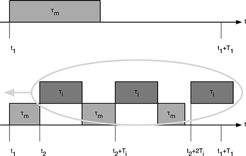
FIGURE 12.2
Interference to τm due to higher-priority tasks τi.
The above argument can finally be repeated for all tasks τi;1 ≤ i < m, thus proving the theorem.
Under the hypotheses of the theorem, it is possible to check whether or not a given priority assignment scheme will yield a feasible scheduling algorithm without simulating it for the LCM of the periods. If all tasks conclude their execution before the deadline—that is, they all fulfill their deadlines—when they are released simultaneously and therefore are at their critical instant, then the scheduling algorithm is feasible.
What we are going to prove is the optimality of Rate Monotonic in the worst case, that is, for critical instants. Observe that this condition may also not occur since it depends on the initial phases of the tasks, but this fact does not alter the outcome of the following proof. In fact, if a system is schedulable in critical instants, it will remain schedulable for every combination of task phases.
We are now ready to prove the optimality of Rate Monotonic (abbreviated in the following as RM), and we shall do it assuming that all the initial task jobs are released simultaneously at time 0. The optimality of RM is proved by showing that, if a task set is schedulable by an arbitrary (but fixed) priority assignment, then it is also schedulable by RM. This result also implies that if RM cannot schedule a certain task set, no other fixed-priority assignment algorithm can schedule it.
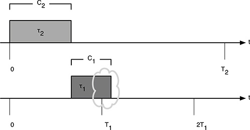
FIGURE 12.3
Tasks τ1 and τ2 not scheduled under RM.
We shall consider first the simpler case in which exactly two tasks are involved, and we shall prove that if the set of two tasks τ1 and τ2 is schedulable by any arbitrary, but fixed, priority assignment, then it is schedulable by RM as well.
Let us consider two tasks, τ1 and τ2, with T1 < T2. If their priorities are not assigned according to RM, then τ2 will have a priority higher than τ1. At a critical instant, their situation is that shown in Figure 12.3.
The schedule is feasible if (and only if) the following inequality is satisfied:
In fact, if the sum of the computation time of τ1 and τ2 is greater than the period of τ1, it is not possible that τ1 can finish its computation within its deadline.
If priorities are assigned according to RM, then task τ1 will have a priority higher than τ2. If we let F be the number of periods of τ1 entirely contained within T2, that is,
then, in order to determine the feasibility conditions, we must consider two cases (which cover all possible situations):
The execution time C1 is “short enough” so that all the instances of τ1 within the critical zone of τ2 are completed before the next release of τ2.
The execution of the last instance of τ1 that starts within the critical zone of τ2 overlaps the next release of τ2.
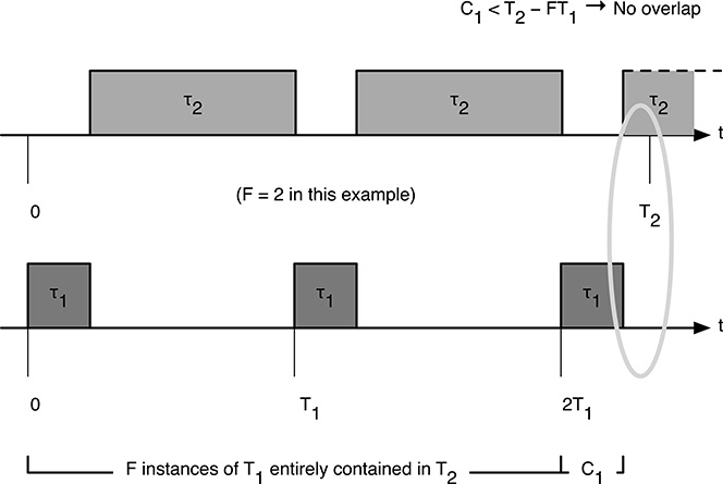
FIGURE 12.4
Situation in which all the instances of τ1 are completed before the next release of τ2.
Let us consider case 1 first, corresponding to Figure 12.4.
The first case occurs when
From Figure 12.4, we can see that the task set is schedulable if and only if
Now consider case 2, corresponding to Figure 12.5. The second case occurs when
From Figure 12.5, we can see that the task set is schedulable if and only if
In summary, given a set of two tasks, τ1 and τ2, with T1 < T2 we have the following two conditions:
When priorities are assigned according to RM, the set is schedulable if and only if
(F + 1)C1 + C2 ≤ T2, when C1 < T2 − FT1.
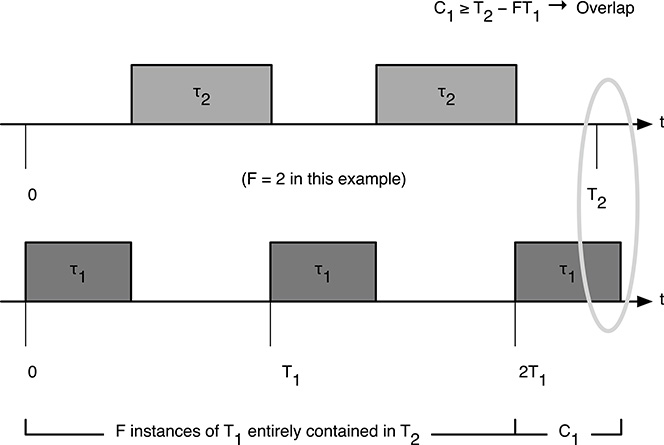
FIGURE 12.5
Situation in which the last instance of τ1 that starts within the critical zone of τ2 overlaps the next release of τ2.FC1 + C2 ≤ FT1, when C1 ≥ T2 − FT1.
When priorities are assigned otherwise, the set is schedulable if and only if C1 + C2 ≤ T1
To prove the optimality of RM with two tasks, we must show that the following two implications hold:
If C1 < T2 − FT1, then C1 + C2 ≤ T1 ⇒ (F +1)C1 + C2 ≤ T2.
If C1 ≥ T2 − FT1, then C1 + C2 ≤ T1 ⇒ FC1 + C2 ≤ FT1.
Consider the first implication: if we multiply both members of C1 + C2 ≤ T1by F and then add C1, we obtain
We know that F ≥ 1 (otherwise, it would not be T1 < T2), and hence,
Moreover, from the hypothesis we have
As a consequence, we have
which proves the first implication.
Consider now the second implication: if we multiply both members of C1 + C2 ≤ T1 by F, we obtain
We know that F ≥ 1 (otherwise, it would not be T1 < T2), and hence
As a consequence, we have
which concludes the proof of the optimality of RM when considering two tasks.
The optimality of RM is then extended to an arbitrary set of tasks thanks to the following theorem [60]:
Theorem 12.2. If the task set τ1,..., τn (n tasks) is schedulable by any arbitrary, but fixed, priority assignment, then it is schedulable by RM as well.
The proof is a direct consequence of the previous considerations: let τi and τj be two tasks of adjacent priorities, τi being the higher-priority one, and suppose that Ti > Tj. Having adjacent priorities, both τi and τj are affected in the same way by the interferences coming from the higher-priority tasks (and not at all by the lower-priority ones). Hence, we can apply the result just obtained and state that if we interchange the priorities of τi and τj, the set is still schedulable. Finally, we notice that the RM priority assignment can be obtained from any other priority assignment by a sequence of pairwise priority reorderings as above, thus ending the proof.
The above problem has far-reaching implications because it gives us a simple way for assigning priorities to real-time tasks knowing that that choice is the best ever possible. At this point we may wonder if it is possible to do better by relaxing the fixed-priority assumption. From the discussion at the beginning of this chapter, the reader may have concluded that dynamic priority should be abandoned when dealing with real-time systems. This is true for the priority assignment algorithms that are commonly used in general purpose operating systems since there is no guarantee that a given job will terminate within a fixed amount of time. There are, however, other algorithms for assigning priority to tasks that do not only ensure a timely termination of the job execution but perform better than fixed-priority scheduling. The next section will introduce the Earliest Deadline First dynamic priority assignment policy, which takes into account the absolute deadline of every task in the priority assignment.
12.3 The Earliest Deadline First Scheduler
The Earliest Deadline First (abbreviated as EDF) algorithm selects tasks according to their absolute deadlines. That is, at each instant, tasks with earlier deadlines will receive higher priorities. Recall that the absolute deadline di,j of the j-th instance (job) of the task τi is formally
where ϕi is the phase of task τi, that is, the release time of its first instance (for which j = 0), and Ti and Di are the period and relative deadlines of task τi, respectively. The priority of each task is assigned dynamically, because it depends on the current deadlines of the active task instances. The reader may be concerned about the practical implementation of such dynamic priority assignment: does it require that the scheduler must continuously monitor the current situation in order to arrange task priorities when needed? Luckily, the answer is no: in fact, task priorities may be updated only when a new task instance is released (task instances are released at every task period). Afterwards, when time passes, the relative order due to the proximity in time of the next deadline remains unchanged among active tasks, and therefore, priorities are not changed.
As for RM, EDF is an intuitive choice as it makes sense to increase the priority of more “urgent” tasks, that is, for which deadline is approaching. We already stated that intuition is not a mathematical proof, therefore we need a formal way of proving that EDF is the optimal scheduling algorithm, that is, if any task set is schedulable by any scheduling algorithm, then it is also schedulable by EDF. This fact can be proved under the following assumption:
Tasks are scheduled preemptively;
There is only one processor.
The formal proof will be provided in the next chapter, where it will be shown that any set of tasks whose processor utilization does not exceed the processor capability is schedulable under EDF. The processor utilization for a set of tasks τ1,..., τn is formally defined as
where each term represents the fraction of processor time devoted to task τi. Clearly, it is not possible to schedule on a single processor a set of tasks for which the above sum is larger than one (in other words, processor utilization cannot be larger than 100%). Otherwise, the set of tasks will be in any case schedulable under EDF.
12.4 Summary
This chapter has introduced the basics of task based scheduling, providing two “optimal” scheduling procedures: RM for fixed task priority assignment, and EDF for dynamic task priority assignment. Using a fixed-priority assignment has several advantages over EDF, among which are the following:
Fixed-priority assignment is easier to implement than EDF, as the scheduling attribute (priority) is static.
EDF requires a more complex run-time system, which will typically have a higher overhead.
During overload situations, the behavior of fixed-priority assignment is easier to predict (the lower-priority processes will miss their deadlines first).
EDF is less predictable and can experience a domino effect in which a large number of tasks unnecessarily miss their deadline.
On the other side, EDF is always able to exploit the full processor capacity, whereas fixed-priority assignment, and therefore RM, in the worst case does not.
EDF implementations are not common in commercial real-time kernels because the operating system would need to keep into account a set of parameters that is not considered in general-purpose operating systems. Moreover, EDF refers to a task model (periodic tasks with given deadline) that is more specific than the usual model of process. There is, however, a set of real-time open-source kernels that support EDF scheduling, and a new scheduling mode has been recently proposed for Linux [29]. Both have developed under the FP7 European project ACTORS [1].
Here, each task is characterized by a budget and a period, which is equal to its relative deadline. At any time, the system schedules the ready tasks having the earliest deadlines. During execution, the budget is decreased at every clock tick, and when a task’s budget reaches zero (i.e., the task executed for a time interval equal to its budget), the task is stopped until the beginning of the next period, the deadline of the other tasks changed accordingly, and the task with the shortest deadline chosen for execution.
Up to now, however, the usage of EDF scheduling is not common in embedded systems, and a fixed task priority under RM policy is normally used.
As a final remark, observe that all the presented analysis relies on the assumption that the considered tasks do not interact each other, neither are they suspended, for example, due to an I/O operation. This is a somewhat unrealistic assumption (whole chapters of this book are devoted to interprocess communication and I/O), and such effects must be taken into consideration in real-world systems. This will be the main argument of Chapters 15 and 16, which will discuss the impact in the schedulability analysis of the use of system resources and I/O operations.