
2
A Case Study: Vision Control
CONTENTS
2.1.1 Accessing the I/O Registers
2.1.3 Direct Memory Access (DMA)
2.2 Input/Output Operations and the Operating System
2.2.2 Input/Output Abstraction in Linux
2.3 Acquiring Images froma Camera Device
2.3.1 Synchronous Read from a Camera Device
2.3.3 Handling Data Streaming from the Camera Device
This chapter describes a case study consisting of an embedded application performing online image processing. Both theoretical and practical concepts are introduced here: after an overview of basic concepts in computer input/output, some important facts on operating systems (OS) and software complexity will be presented here. Moreover, some techniques for software optimization and parallelization will be presented and discussed in the framework of the presented case study. The theory and techniques that are going to be introduced do not represent the main topic of this book. They are necessary, nevertheless, to fully understand the remaining chapters, which will concentrate on more specific aspects such as multithreading and process scheduling.
The presented case study consists of a Linux application that acquires a sequence of images (frames) from a video camera device. The data acquisition program will then perform some elaboration on the acquired images in order to detect the coordinates of the center of a circular shape in the acquired images.
This chapter is divided into four main sections. In the first section general concepts in computer input/output (I/O) are presented. The second section will discuss how I/O is managed by operating systems, in particular Linux, while in the third one the implementation of the frame acquisition is presented. The fourth section will concentrate on the analysis of the acquired frames to retrieve the desired information; after presenting two widespread algorithms for image analysis, the main concepts about software complexity will be presented, and it will be shown how the execution time for those algorithms can be reduced, sometimes drastically, using a few optimization and parallelization techniques.
Embedded systems carrying out online analysis of acquired images are becoming widespread in industrial control and surveillance. In order to acquire the sequence of the frames, the video capture application programming interface for Linux (V4L2) will be used. This interface supports most commercial USB webcams, which are now ubiquitous in laptops and other PCs. Therefore this sample application can be easily reproduced by the reader, using for example his/her laptop with an integrated webcam.
2.1 Input Output on Computers
Every computer does input/output (I/O); a computer composed only of a processor and the memory would do barely anything useful, even if containing all the basic components for running programs. I/O represents the way computers interact with the outside environment. There is a great variety of I/O devices: A personal computer will input data from the keyboard and the mouse, and output data to the screen and the speakers while using the disk, the network connection, and the USB ports for both input and output. An embedded system typically uses different I/O devices for reading data from sensors and writing data to actuators, leaving user interaction be handled by remote clients connected through the local area network (LAN).
2.1.1 Accessing the I/O Registers
In order to communicate with I/O devices, computer designers have followed two different approaches: dedicated I/O bus and memory-mapped I/O. Every device defines a set of registers for I/O management. Input registers will contain data to be read by the processor; output registers will contain data to be outputted by the device and will be written by the processor; status registers will contain information about the current status of the device; and finally control registers will be written by the processor to initiate or terminate device activities.
When a dedicated bus is defined for the communication between the processor and the device registers, it is also necessary that specific instructions for reading or writing device register are defined in the set of machine instructions. In order to interact with the device, a program will read and write appropriate values onto the I/O bus locations (i.e., at the addresses corresponding to the device registers) via specific I/O Read and Write instructions.
In memory-mapped I/O, devices are seen by the processor as a set of registers, but no specific bus for I/O is defined. Rather, the same bus used to exchange data between the processor and the memory is used to access I/O devices. Clearly, the address range used for addressing device registers must be disjoint from the set of addresses for the memory locations. Figure 2.1 and Figure 2.2 show the bus organization for computers using a dedicated I/O bus and memory-mapped I/O, respectively. Memory-mapped architectures are more common nowadays, but connecting all the external I/O devices directly to the memory bus represents a somewhat simplified solution with several potential drawbacks in reliability and performance. In fact, since speed in memory access represents one of the major bottlenecks in computer performance, the memory bus is intended to operate at a very high speed, and therefore it has very strict constraints on the electrical characteristics of the bus lines, such as capacity, and in their dimension. Letting external devices be directly connected to the memory bus would increase the likelihood that possible malfunctions of the connected devices would seriously affect the function of the whole system and, even if that were not the case, there would be the concrete risk of lowering the data throughput over the memory bus.
In practice, one or more separate buses are present in the computer for I/O, even with memory-mapped architectures. This is achieved by letting a bridge component connect the memory bus with the I/O bus. The bridge presents itself to the processor as a device, defining a set of registers for programming the way the I/O bus is mapped onto the memory bus. Basically, a bridge can be programmed to define one or more address mapping windows. Every address mapping window is characterized by the following parameters:
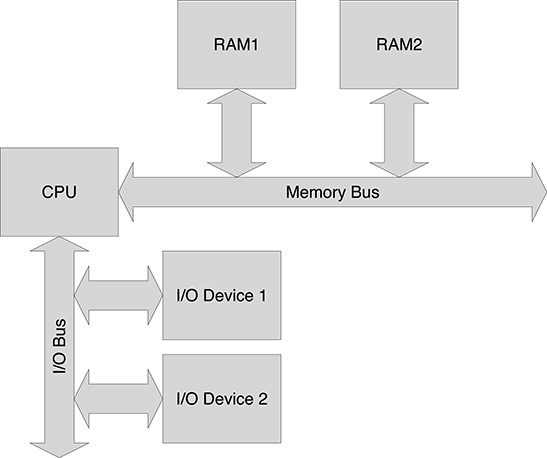
FIGURE 2.1
Bus architecture with a separate I/O bus.
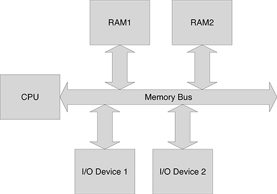
FIGURE 2.2
Bus architecture for Memory Mapped I/O.
Start and end address of the window in the memory bus
Mapping address offset
Once the bridge has been programmed, for every further memory access performed by the processor whose address falls in the selected address range, the bridge responds in the bus access protocol and translates the read or write operation performed in the memory bus into an equivalent read or write operation in the I/O bus. The address used in the I/O bus is obtained by adding the preprogrammed address offset for that mapping window. This simple mechanism allows to decouple the addresses used by I/O devices over the I/O bus from the addresses used by the processor.
A common I/O bus in computer architectures is the Peripheral Component Interconnect (PCI) bus, widely used in personal computers for connecting I/O devices. Normally, more than one PCI segment is defined in the same computer board. The PCI protocol, in fact, poses a limit in the number of connected devices and, therefore, in order to handle a larger number of devices, it is necessary to use PCI to PCI bridges, which connect different segments of the PCI bus. The bridge will be programmed in order to define map address windows in the primary PCI bus (which sees the bridge as a device connected to the bus) that are mapped onto the corresponding address range in the secondary PCI bus (for which the bridge is the master, i.e., leads bus operations). Following the same approach, new I/O buses, such as the Small Computer System Interface (SCSI) bus for high-speed disk I/O, can be integrated into the computer board by means of bridges connecting the I/O bus to the memory bus or, more commonly, to the PCI bus. Figure 2.3 shows an example of bus configuration defining a memory to PCI bridge, a PCI to PCI bridge, and a PCI to SCSI bridge.
One of the first actions performed when a computer boots is the configuration of the bridges in the system. Firstly, the bridges directly connected to the memory bus are configured, so that the devices over the connected buses can be accessed, including the registers of the bridges connecting these to new I/O buses. Then the bridges over these buses are configured, and so on. When all the bridges have been properly configured, the registers of all the devices in the system are directly accessible by the processor at given addresses over the memory bus. Properly setting all the bridges in the system may be tricky, and a wrong setting may make the system totally unusable. Suppose, for example, what could happen if an address map window for a bridge on the memory bus were programmed with an overlap with the address range used by the RAM memory. At this point the processor would be unable to access portions of memory and therefore would not anymore be able to execute programs.
Bridge setting, as well as other very low-level configurations are normally performed before the operating system starts, and are carried out by the Basic Input/Output System (BIOS), a code which is normally stored on ROM and executed as soon as the computer is powered. So, when the operating system starts, all the device registers are available at proper memory addresses. This is, however, not the end of the story: in fact, even if device registers are seen by the processor as if they were memory locations, there is a fundamental difference between devices and RAM blocks. While RAM memory chips are expected to respond in a time frame on the order of nanoseconds, the response time of devices largely varies and in general can be much longer. It is therefore necessary to synchronize the processor and the I/O devices.
2.1.2 Synchronization in I/O
Consider, for example, a serial port with a baud rate of 9600 bit/s, and suppose that an incoming data stream is being received; even if ignoring the protocol overhead, the maximum incoming byte rate is 1200 byte/s. This means that the computer has to wait 0.83 milliseconds between two subsequent incoming bytes. Therefore, a sort of synchronization mechanism is needed to let the computer know when a new byte is available to be read in a data register for readout. The simplest method is polling, that is, repeatedly reading a status register that indicates whether new data is available in the data register. In this way, the computer can synchronize itself with the actual data rate of the device. This comes, however, at a cost: no useful operation can be carried out by the processor when synchronizing to devices in polling. If we assume that 100 ns are required on average for memory access, and assuming that access to device registers takes the same time as a memory access (a somewhat simplified scenario since we ignore here the effects of the memory cache), acquiring a data stream from the serial port would require more than 8000 read operations of the status register for every incoming byte of the stream – that is, wasting 99.99% of the processor power in useless accesses to the status register. This situation becomes even worse for slower devices; imagine the percentage of processor power for doing anything useful if polling were used to acquire data from the keyboard!
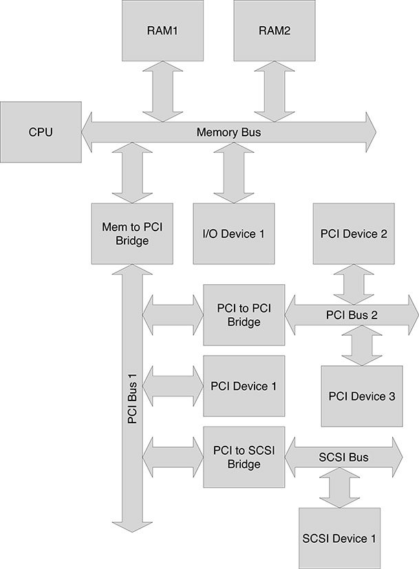
FIGURE 2.3
Bus architecture with two PCI buses and one SCSI bus.
Observe that the operations carried out by I/O devices, once programmed by a proper configuration of the device registers, can normally proceed in parallel with the execution of programs. It is only required that the device should notify the processor when an I/O operation has been completed, and new data can be read or written by the processor. This is achieved using Interrupts, a mechanism supported by most I/O buses. When a device has been started, typically by writing an appropriate value in a command register, it proceeds on its own. When new data is available, or the device is ready to accept new data, the device raises an interrupt request to the processor (in most buses, some lines are dedicated to interrupt notification) which, as soon as it finishes executing the current machine instruction, will serve the interrupt request by executing a specific routine, called Interrupt Service Routine (ISR), for the management of the condition for which the interrupt has been generated.
Several facts must be taken into account when interrupts are used to synchronize the processor and the I/O operations. First of all, more than one device could issue an interrupt at the same time. For this reason, in most systems, a priority is associated with interrupts. Devices can in fact be ranked based on their importance, where important devices require a faster response. As an example, consider a system controlling a nuclear plant: An interrupt generated by a device monitoring the temperature of a nuclear reactor core is for sure more important than the interrupt generated by a printer device for printing daily reports. When a processor receives an interrupt request with a given associated priority level N, it will soon respond to the request only if it is not executing any service routine for a previous interrupt of priority M, M ≥ N. In this case, the interrupt request will be served as soon as the previous Interrupt Service Routine has terminated and there are no pending interrupts with priority greater or equal to the current one.
When a processor starts serving an interrupt, it is necessary that it does not lose information about the program currently in execution. A program is fully described by the associated memory contents (the program itself and the associated data items), and by the content of the processor registers, including the Program Counter (PC), which records the address of the current machine instruction, and the Status Register (SR), which contains information on the current processor status. Assuming that memory locations used to store the program and the associated data are not overwritten during the execution of the interrupt service routine, it is only necessary to preserve the content of the processor registers. Normally, the first actions of the routine are to save in the stack the content of the registers that are going to be used, and such registers will be restored just before its termination. Not all the registers can be saved in this way; in particular, the PC and the SR are changed just before starting the execution of the interrupt service routine. The PC will be set to the address of the first instruction of the routine, and the SR will be updated to reflect the fact that the process is starting to service an interrupt of a given priority. So it is necessary that these two register are saved by the processor itself and restored when the interrupt service routine has finished (a specific instruction to return from ISR is defined in most computer architectures). In most architectures the SR and PC registers are saved on the stack, but others, such as the ARM architecture, define specific registers to hold the saved values.
A specific interrupt service routine has to be associated with every possible source of interrupt, so that the processor can take the appropriate actions when an I/O device generates an interrupt request. Typically, computer architectures define a vector of addresses in memory, called a Vector Table, containing the start addresses of the interrupt service routines for all the I/O devices able to generate interrupt requests. The offset of a given ISR within the vector table is called the Interrupt Vector Number. So, if the interrupt vector number were communicated by the device issuing the interrupt request, the right service routine could then be called by the processor. This is exactly what happens; when the processor starts serving a given interrupt, it performs a cycle on the bus called the Interrupt Acknowledge Cycle (IACK) where the processor communicates the priority of the interrupt being served, and the device which issued the interrupt request at the specified priority returns the interrupt vector number. In case two different devices issued an interrupt request at the same time with the same priority, the device closest to the processor in the bus will be served. This is achieved in many buses by defining a bus line in Daisy Chain configuration, that is, which is propagated from every device to the next one along the bus, only in cases where it did not answer to an IACK cycle. Therefore, a device will answer to an IACK cycle only if both conditions are met:
It has generated a request for interrupt at the specified priority
It has received a signal over the daisy chain line
Note that in this case it will not propagate the daisy chain signal to the next device.
The offset returned by the device in an IACK cycle depends on the current organization of the vector table and therefore must be a programmable parameter in the device. Typically, all the devices which are able to issue an interrupt request have two registers for the definition of the interrupt priority and the interrupt vector number, respectively. The sequence of actions is shown in Figure 2.4, highlighting the main steps of the sequence:
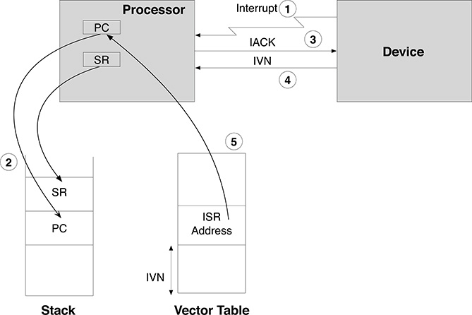
FIGURE 2.4
The Interrupt Sequence.
The device issues an interrupt request;
The processor saves the context, i.e., puts the current values of the PC and of the SR on the stack;
The processor issues an interrupt acknowledge cycle (IACK) on the bus;
The device responds by putting the interrupt vector number (IVN) over the data lines of the bus;
The processor uses the IVN as an offset in the vector table and loads the interrupt service routine address in the PC.
Programming a device using interrupts is not a trivial task, and it consists of the following steps:
The interrupt service routine has to be written. The routine can assume that the device is ready at the time it is called, and therefore no synchronization (e.g., polling) needs to be implemented;
During system boot, that is when the computer and the connected I/O devices are configured, the code of the interrupt service routine has to be loaded in memory, and its start address written in the vector table at, say, offset N;
The value N has to be communicated to the device, usually written in the interrupt vector number register;
When an I/O operation is requested by the program, the device is started, usually by writing appropriate values in one or more command registers. At this point the processor can continue with the program execution, while the device operates. As soon as the device is ready, it will generate an interrupt request, which will be eventually served by the processor by running the associated interrupt service routine.
In this case it is necessary to handle the fact that data reception is asynchronous. A commonly used techniques is to let the program continue after issuing an I/O request until the data received by the device is required. At this point the program has to suspend its execution waiting for data, unless not already available, that is, waiting until the corresponding interrupt service routine has been executed. For this purpose the interprocess communication mechanisms described in Chapter 5 will be used.
2.1.3 Direct Memory Access (DMA)
The use of interrupts for synchronizing the processor and the connected I/O devices is ubiquitous, and we will see in the next chapters how interrupts represent the basic mechanism over which operating systems are built. Using interrupts clearly spares processor cycles when compared with polling; however, there are situations in which even interrupt-driven I/O would require too much computing resources. To better understand this fact, let’s consider a mouse which communicates its current position by interrupting the processor 30 times per second. Let’s assume that 400 processor cycles are required for the dispatching of the interrupt and the execution of the interrupt service routine. Therefore, the number of processor cycles which are dedicated to the mouse management per second is 400 ∗ 30 = 12000. For a 1 GHz clock, the fraction of processor time dedicated to the management of the mouse is 12000/109, that is, 0.0012% of the processor load. Managing the mouse requires, therefore, a negligible fraction of processor power.
Consider now a hard disk that is able to read data with a transfer rate of 4 MByte/s, and assume that the device interrupts the processor every time 16 bytes of data are available. Let’s also assume that 400 clock cycles are still required to dispatch the interrupt and execute the associated service routine. The device will therefore interrupt the processor 250000 times per second, and 108 processor cycles will be dedicated to handle data transfer every second. For a 1 GHz processor this means that 10% of the processor time is dedicated to data transfer, a percentage clearly no more acceptable.
Very often data exchanged with I/O devices are transferred from or to memory. For example, when a disk block is read it is first transferred to memory so that it is later available to the processor. If the processor itself were in charge of transferring the block, say, after receiving an interrupt request from the disk device to signal the block availability, the processor would repeatedly read data items from the device’s data register into an internal processor register and write it back into memory. The net effect is that a block of data has been transferred from the disk into memory, but it has been obtained at the expense of a number of processor cycles that could have been used to do other jobs if the device were allowed to write the disk block into memory by itself. This is exactly the basic concept of Direct Memory Access (DMA), which is letting the devices read and write memory by themselves so that the processor will handle I/O data directly in memory. In order to put this simple concept in practice it is, however, necessary to consider a set of facts. First of all, it is necessary that the processor can “program” the device so that it will perform the correct actions, that is, reading/writing a number N of data items in memory, starting from a given memory address A. For this purpose, every device able to perform DMA provides at least the following registers:
A Memory Address Register (MAR) initially containing the start address in memory of the block to be transferred;
A Word Count register (WC) containing the number of data items to be transferred.
So, in order to program a block read or write operation, it is necessary that the processor, after allocating a block in memory and, in case of a write operation, filling it with the data to be output to the device, writes the start address and the number of data items in the MAR and WC registers, respectively. Afterwards the device will be started by writing an appropriate value in (one of) the command register(s). When the device has been started, it will operate in parallel with the processor, which can proceed in the execution of the program. However, as soon as the device is ready to transfer a data item, it will require the memory bus used by the processor to exchange data with memory, and therefore some sort of bus arbitration is needed since it is not possible that two devices read or write the memory at the same time on the same bus (note however that nowadays memories often provide multiport access, that is, allow simultaneous access to different memory addresses). At any time one, and only one, device (including the processor) connected to the bus is the master, i.e., can initiate a read or write operation. All the other connected devices at that time are slaves and can only answer to a read/write bus cycle when they are addressed. The memory will be always a slave in the bus, as well as the DMA-enabled devices when they are not performing DMA. At the time such a device needs to exchange data with the memory, it will ask the current master (normally the processor, but it may be another device performing DMA) the ownership of the bus. For this purpose the protocol of every bus able to support ownership transfer is to define a cycle for the bus ownership transfer. In this cycle, the potential master raises a request line and the current master, in response, relinquishes the mastership, signaling this over another bus line, and possibly waiting for the termination of a read/write operation in progress. When a device has taken the bus ownership, it can then perform the transfer of the data item and will remain the current master until the processor or another device asks to become the new master. It is worth noting that the bus ownership transfers are handled by the bus controller components and are carried out entirely in hardware. They are, therefore, totally transparent to the programs being executed by the processor, except for a possible (normally very small) delay in their execution.
Every time a data item has been transferred, the MAR is incremented and the WC is decremented. When the content of the WC becomes zero, all the data have been transferred, and it is necessary to inform the processor of this fact by issuing an interrupt request. The associated Interrupt Service Routine will handle the block transfer termination by notifying the system of the availability of new data. This is normally achieved using the interprocess communication mechanisms described in Chapter 5.
2.2 Input/Output Operations and the Operating System
After having seen the techniques for handling I/O in computers, the reader will be convinced that it is highly desirable that the complexity of I/O should be handled by the operating system and not by user programs. Not surprisingly, this is the case for most operating systems, which offer a unified interface for I/O operations despite the large number of different devices, each one defining a specific set of registers and requiring a specific I/O protocol. Of course, it is not possible that operating systems could include the code for handling I/O in every available device. Even if it were the case, and the developers of the operating system succeed in the titanic effort of providing the device specific code for every known device, the day after the system release there will be tens of new devices not supported by such an operating system. For this reason, operating systems implement the generic I/O functionality, but leave the details to a device-specific code, called the Device Driver. In order to be integrated into the system, every device requires its software driver, which depends not only on the kind of hardware device but also on the operating system. In fact, every operating system defines its specific set of interfaces and rules a driver must adhere to in order to be integrated. Once installed, the driver becomes a component of the operating system. This means that a failure in the device driver code execution becomes a failure of the operating system, which may lead to the crash of the whole system. (At least in monolithic operating systems such as Linux and Windows; this may be not true for other systems, such as microkernel-based ones.) User programs will never interact directly with the driver as the device is accessible only via the Application Programming Interface (API) provided by the operating system. In the following we shall refer to the Linux operating systems and shall see how a uniform interface can be adapted to the variety of available devices. The other operating systems adopt a similar architecture for I/O, which typically differ only by the name and the arguments of the I/O systems routines, but not on their functionality.
2.2.1 User and Kernel Modes
We have seen how interacting with I/O devices means reading and writing into device registers, mapped at given memory addresses. It is easy to guess what could happen if user programs were allowed to read and write at the memory locations corresponding to device registers. The same consideration holds also for the memory structures used by the operating system itself. If user programs were allowed to freely access the whole addressing range of the computer, an error in a program causing a memory access to a wrong address (something every C programmer experiences often) may lead to the corruption of the operating system data structures, or to an interference with the device operation, leading to a system crash.
For this reason most processors define at least two levels of execution: user mode and kernel (or supervisor) mode. When operating in user mode, a program is not allowed to execute some machine instructions (called Privileged Instructions) or to access sets of memory addresses. Conversely, when operating in kernel mode, a program has full access to the processor instructions and to the full addressing range. Clearly, most of the operating system code will be executed in kernel mode, while user programs are kept away from dangerous operations and are intended to be executed in user mode. Imagine what would happen if the HALT machine instruction for stopping the processor were available in user mode, possibly on a server with tens of connected users.
A first problem arises when considering how a program can switch from user to kernel mode. If this were carried out by a specific machine instruction, would such an instruction be accessible in user mode? If not, it would be useless, but if it were, the barrier between kernel mode and user mode would be easily circumvented, and malicious programs could easily take the whole system down.
So, how to solve the dilemma? The solution lies in a new mechanism for the invocation of software routines. In the normal routine invocation, the calling program copies the arguments of the called routine over the stack and then puts the address of the first instruction of the routine into the Program Counter register, after having copied on the stack the return address, that is, the address of the next instruction in the calling program. Once the called routine terminates, it will pick the saved return address from the stack and put it into the Program Counter, so that the execution of the calling program is resumed. We have already seen, however, how the interrupt mechanism can be used to “invoke” an interrupt service routine. In this case the sequence is different, and is triggered not by the calling program but by an external hardware device. It is exactly when the processor starts executing an Interrupt Service routine that the current execution mode is switched to kernel mode. When the interrupt service routine returns and the interrupted program resumes its execution, unless not switching to a new interrupt service routine, the execution mode is switched to user mode. It is worth noting that the mode switch is not controlled by the software, but it is the processor which only switches to kernel mode when servicing an interrupt.
This mechanism makes sense because interrupt service routines interact with devices and are part of the device driver, that is, of a software component that is integrated in the operating system. However, it may happen that user programs have to do I/O operations, and therefore they need to execute some code in kernel mode. We have claimed that all the code handling I/O is part of the operating system and therefore the user program will call some system routine for doing I/O. However, how do we switch to kernel mode in this case where the trigger does not come from an hardware device? The solution is given by Software Interrupts. Software interrupts are not triggered by an external hardware signal, but by the execution of a specific machine instruction. The interrupt mechanism is quite the same: The processor saves the current context, picks the address of the associated interrupt service routine from the vector table and switches to kernel mode, but in this case the Interrupt Vector number is not obtained by a bus IACK cycle; rather, it is given as an argument to the machine instruction for the generation of the software interrupt.
The net effect of software interrupts is very similar to that of a function call, but the underlying mechanism is completely different. This is the typical way the operating system is invoked by user programs when requesting system services, and it represents an effective barrier protecting the integrity of the system. In fact, in order to let any code to be executed via software interrupts, it is necessary to write in the vector table the initial address of such code but, not surprisingly, the vector table is not accessible in user mode, as it belongs to the set of data structures whose integrity is essential for the correct operation of the computer. The vector table is typically initialized during the system boot (executed in kernel mode) when the operating system initializes all its data structures.
To summarize the above concepts, let’s consider the execution story of one of the most used C library function: printf(), which takes as parameter the (possibly formatted) string to be printed on the screen. Its execution consists of the following steps:
The program calls routine
printf(), provided by the C run time library. Arguments are passed on the stack and the start address of theprintfroutine is put in the program counter;The
printfcode will carry out the required formatting of the passed string and the other optional arguments, and then calls the operating system specific system service for writing the formatted string on the screen;The system routine executes initially in user mode, makes some preparatory work and then needs to switch in kernel mode. To do this, it will issue a software interrupt, where the passed interrupt vector number specifies the offset in the Vector Table of the corresponding ISR routine to be executed in kernel mode;
The ISR is eventually activated by the processor in response to the software interrupt. This routine is provided by the operating system and it is now executing in kernel mode;
After some work to prepare the required data structures, the ISR routine will interact with the output device. To do this, it will call specific routines of the device driver;
The activated driver code will write appropriate values in the device registers to start transferring the string to the video device. In the meantime the calling process is put in wait state (see Chapter 3 for more information on processes and process states);
A sequence of interrupts will be likely generated by the device to handle the transfer of the bytes of the string to be printed on the screen;
When the whole string has been printed on the screen, the calling process will be resumed by the operating system and
printfwill return.
Software interrupts provide the required barrier between user and kernel mode, which is of paramount importance in general purpose operating systems. This comes, however, at a cost: the activation of a kernel routine involves a sequence of actions, such as saving the context, which is not necessary in a direct call. Many embedded systems are then not intended to be of general usage. Rather, they are intended to run a single program for control and supervision or, in more complex systems involving multitasking, a well defined set of programs developed ad hoc. For this reason several real-time operating systems do not support different execution levels (even if the underlying hardware could), and all the software is executed in kernel mode, with full access to the whole set of system resources. In this case, a direct call is used to activate system routines. Of course, the failure of a program will likely bring the whole system down, but in this case it is assumed that the programs being executed have already been tested and can therefore be trusted.
2.2.2 Input/Output Abstraction in Linux
Letting the operating system manage input/output on behalf of the user is highly desirable, hiding as far as possible the communication details and providing a simple and possibly uniform interface for I/O operations. We shall learn how a simple Application Programming Interface for I/O can be effectively used despite the great variety of devices and of techniques for handling I/O. Here we shall refer to Linux, but the same concepts hold for the vast majority of the other operating systems.
In Linux every I/O device is basically presented to users as a file. This may seem at a first glance a bit surprising since the similarity between files and devices is not so evident, but the following considerations hold:
In order to be used, a file must be open. The
open()system routine will create a set of data structures that are required to handle further operations on that file. A file identifier is returned to be used in the following operations for that file in order to identify the associated data structures. In general, every I/O device requires some sort of initialization before being used. Initialization will consist of a set of operations performed on the device and in the preparation of a set of support data structures to be used when operating on that device. So anopen()system routine makes sense also for I/O devices. The returned identifier (actually an integer number in Linux) is called a Device Descriptor and uniquely identifies the device instance in the following operations. When a file is no more used, it is closed and the associated data structures deallocated. Similarly, when a I/O device is no more used, it will be closed, performing cleanup operations and freeing the associated resources.A file can be read or written. In the read operation, data stored in the file are copied in the computer memory, and the converse holds for write operations. Regardless of the actual nature of a I/O device, there are two main categories of interaction with the computer: read and write. In read operation, data from the device is copied into the computer memory to be used by the program. In write operations, data in memory will be transferred to the device. Both
read()andwrite()system routines will require the target file or device to be uniquely identified. This will be achieved by passing the identifier returned by theopen()routine.
However, due to the variety of hardware devices that can be connected to a computer, it is not always possible to provide a logical mapping of the device’s functions exclusively into read-and-write operations. Consider, as an example, a network card: actions such as receiving data and sending data over the network can be mapped into read-and-write operations, respectively, but others, like the configuration of the network address, require a different interface. In Linux this is achieved by providing an additional routine for I/O management: ioctl(). In addition to the device descriptor, ioctl() defines two more arguments: the first one is an integer number and is normally used to specify the kind of operation to be performed; the second one is a pointer to a data structure that is specific to the device and the operation. The actual meaning of the last argument will depend on the kind of device and on the specified kind of operation. It is worth noting that Linux does not make any use of the last two ioctl() arguments, passing them as they are to the device-specific code, i.e., the device driver.
The outcome of the device abstraction described above is deceptively simple: the functionality of all the possible devices connected to the computers is basically carried out by the following four routines:
open()to initialize the device;close()to close and release the device;read()to get data from the device;write()to send data to the device;ioctl()for all the remaining operations of the device.
The evil, however, hides in the details, and in fact all the complexity in the device/computer interaction has been simply moved to ioctl(). Depending on the device’s nature, the set of operations and of the associated data structures may range from a very few and simple configurations to a fairly complex set of operations and data structures, described by hundreds of user manual pages. This is exactly the case of the standard driver for the camera devices that will be used in the subsequent sections of this chapter for the presented case study.
The abstraction carried out by the operating system in the application programming interface for device I/O is also maintained in the interaction between the operating system and the device-specific driver. We have already seen that, in order to integrate a device in the systems, it is necessary to provide a device-specific code assembled into the device driver and then integrated into the operating system. Basically, a device driver provides the implementation of the open, close, read, write, and ioctl operations. So, when a program opens a device by invoking the open() system routine, the operating system will first carry out some generic operations common to all devices, such as the preparation of its own data structures for handling the device, and will then call the device driver’s open() routine to carry out the required device specific actions. The actions carried out by the operating system may involve the management of the calling process. For example, in a read operation, the operating system, after calling the device-specific read routine, may suspend the current process (see Chapter 3 for a description of the process states) in the case the required data are not currently available. When the data to be read becomes available, the system will be notified of it, say, with an interrupt from the device, and the operating system will wake the process that issued the read() operation, which can now terminate the read() system call.
2.3 Acquiring Images from a Camera Device
So far, we have learned how input/output operation are managed by Linux. Here we shall see in detail how the generic routines for I/O can be used for a real application, that is, acquiring images from a video camera device. A wide range of camera devices is available, ranging from $10 USB Webcams to $100K cameras for ultra-fast image recording. The number and the type of configuration parameters varies from device to device, but it will always include at least:
Device capability configuration parameters, such as the ability of supporting data streaming and the supported pixel formats;
Image format definition, such as the width and height of the frame, the number of bytes per line, and the pixel format.
Due to the large number of different camera devices available on the market, having a specific driver for every device, with its own configuration parameters and ioctl() protocol (i.e., the defined operations and the associated data structures), would complicate the life of the programmers quite a lot. Suppose, for example, what would happen if in an embedded system for on-line quality control based on image analysis the type of used camera is changed, say, because a new better device is available. This would imply re-writing all the code which interacts with the device. For this reason, a unified interface to camera devices has been developed in the Linux community. This interface, called V4L2 (Video for Linux Two), defines a set of ioctl operations and associated data structures that are general enough to be adapted for all the available camera devices of common usage. If the driver of a given camera device adheres to the V4L2 standards, the usability of such device is greatly improved and it can be quickly integrated into existing systems. V4L2 improves also interchangeability of camera devices in applications. To this purpose, an important feature of V4L2 is the availability of query operations for discovering the supported functionality of the device. A well-written program, first querying the device capabilities and then selecting the appropriate configuration, can the be reused for a different camera device with no change in the code.
As V4L2 in principle covers the functionality of all the devices available on the market, the standard is rather complicated because it has to foresee even the most exotic functionality. Here we shall not provide a complete description of V4L2 interface, which can be found in [77], but will illustrate its usage by means of two examples. In the first example, a camera device is inquired in order to find out the supported formats and to check whether the YUYV format is supported. If this format is supported, camera image acquisition is started using the read() system routine. YUYV is a format to encode pixel information expressed by the following information:
Luminance (Y)
Blue Difference Chrominance (Cb)
Red Difference Chrominance (Cr)
Y, Cb, and Cr represent a way to encode RGB information in which red (R), green (G), and blue (B) light are added together to reproduce a broad array of colors for image pixels, and there is a precise mathematical relationship between R, G, B, and Y, Cb and Cr parameters, respectively. The luminance Y represents the brightness in an image and can be considered alone if only a grey scale representation of the image is needed. In our case study we are not interested in the colors of the acquired images, rather we are interested in retrieving information from the shape of the objects in the image, so we shall consider only the component Y.
The YUYV format represents a compressed version of the Y, Cb, and Cr. In fact, while the luminance is encoded for every pixel in the image, the chrominance values are encoded for every two pixels. This choice stems from the fact that the human eye is more sensitive to variation of the light intensity, rather than of the colors components. So in the YUYV format, pixels are encoded from the topmost image line and from the left to the right, and four bytes are used to encode two pixels with the following pattern: Yi, Cbi, Yi+1, Cri. To get the grey scale representation of the acquired image, our program will therefore take the first byte of every pair.
2.3.1 Synchronous Read from a Camera Device
This first example shows how to read from a camera device using synchronous frame readout, that is, using the read() function for reading data from the camera device. Its code is listed below;
# include <fcntl.h>
# include <stdio.h>
# include <stdlib.h>
# include <string.h>
# include <errno.h>
# include <linux/videodev2.h>
# include <asm/unistd.h>
# include <poll.h>
# define MAX_FORMAT  100
# define FALSE   0
# define TRUE   1
# define CHECK_IOCTL_STATUS(message) \
if(status == -1)                      \
{                                      \
     perror (message);                 \
     exit(EXIT_FAILURE);               \
}
main (int  argc, char * argv [])
{
    int fd, idx,  status ;
    int pixelformat;
    int imageSize;
    int width, height ;
    int yuyvFound;
    struct v412_capability  cap;    //Query Capability structure
    struct v412_fmtdesc  fmt;       //Query Format Description structure
    struct v412_format  format ;    //Query Format structure
    char * buf;                     //Image buffer
    fd_set  fds;                    //Select descriptors
    struct timeval tv;              //Timeout specification structure
/* Step 1: Open the device */
    fd = open ("/dev/ video1 ",  O_RDWR);
/* Step 2: Check read/write  capability */
    status = ioctl(fd, VIDIOC_QUERYCAP, &cap);
    CHECK_IOCTL_STATUS(" Error Querying capability")
    if (!(cap. capabilities & V4L2_CAP_READWRITE))
    {
       printf (" Read I/O  NOT  supported
");
       exit(EXIT_FAILURE);
    }
/* Step 3: Check supported formats */
    yuyvFound  = FALSE;
    for(idx = 0; idx < MAX_FORMAT; idx ++)
    {
         fmt.index = idx;
         fmt.type = V4L2_BUF_TYPE_VIDEO_CAPTURE;
         status = ioctl (fd, VIDIOC_ENUM_FMT, &fmt);
         if (status != 0)  break ;
         if (fmt. pixelformat == V4L2_PIX_FMT_YUYV)
         {
              yuyvFound = TRUE;
              break ;
         }
    }
    if (! yuyvFound)
    {
       printf (" YUYV format  not  supported
");
       exit (EXIT_FAILURE);
    }
/* Step 4: Read current format definition */
    memset (&format, 0, sizeof (format));
    format.type = V4L2_BUF_TYPE_VIDEO_CAPTURE;
    status = ioctl (fd, VIDIOC_G_FMT,  &format);
    CHECK_IOCTL_STATUS(" Error Querying Format ")
/* Step 5: Set format fields to desired values: YUYV coding,
   480 lines, 640 pixels per line */
    format.fmt.pix.width = 640;
    format.fmt.pix.height = 480;
    format.fmt.pix.pixelformat = V4L2_PIX_FMT_YUYV;
/* Step 6: Write desired format and check actual image size  */
    status = ioctl (fd, VIDIOC_S_FMT,  &format);
    CHECK_IOCTL_STATUS(" Error Setting    Format ")
    width =  format.fmt.pix.width;                     //Image Width
    height = format.fmt.pix.height;                    //Image Height
    //Total image size in bytes
    imageSize = (unsigned int) format.fmt.pix.sizeimage;
/*  Step 7: Start reading from the camera */
    buf = malloc (imagesize);
    FD_ZERO (&fds);
    FD_SET (fd, &fds);
    tv.tv_sec =  20;
    tv.tv_usec =  0;
    for (;;)
    {
        status = select (1,  &fds, NULL, NULL, &tv);
        if (status ==  -1)
        {
              perror (" Error in Select ");
              exit (EXIT_FAILURE);
        }
        status = read(fd, buf,  imageSize);
        if (status == -1)
        {
              perror (" Error reading buffer ");
              exit (EXIT_FAILURE);
        }
/*  Step 8: Do image processing */
            processImage(buf,  width, height,  imagesize);
   }
}
The first action (step 1)in the program is opening the device. System routine open() looks exactly as an open call for a file. As for files, the first argument is a path name, but in this case such a name specifies the device instance. In Linux the names of the devices are all contained in the /dev directory. The files contained in this directory do not correspond to real files (a Webcam is obviously different from a file), rather, they represent a rule for associating a unique name with each device in the system. In this way it is also possible to discover the available devices using the ls command to list the files contained in a directory. By convention, camera devices have the name /dev/video<n>, so the command ls /dev/video* will show how many camera devices are available in the system. The second argument given to system routine open() specifies the protection associated with that device. In this case the constant O_RDWR specifies that the device can be read and written. The returned value is an integer value that uniquely specifies within the system the Device Descriptor, that is the set of data structures held by Linux to manage this device. This number is then passed to the following ioctl() calls to specify the target device. Step 2 consists in checking whether the camera device supports read-/write operation. The attentive reader may find this a bit strange—how could the image frames be acquired otherwise?—but we shall see in the second example that an alternative way, called streaming, is normally (and indeed most often) provided. This query operation is carried out by the following line:
status = ioctl(fd, VIDIOC_QUERYCAP, &cap);
In the above line the ioctl operation code is given by constant VIDIOC_QUERYCAP (defined, as all the other constants used in the management of the video device, in linux/videodev2.h), and the associated data structure for the pointer argument is of type v412_capability. This structure, documented in the V4L2 API specification, defines, among others, a capability field containing a bit mask specifying the supported capabilities for that device.
Line
if(cap.capabilities & V4L2_CAP_READWRITE)
will let the program know whether read/write ability is supported by the device.
In step 3 the device is queried about the supported pixel formats. To do this, ioctl() is repeatedly called, specifying VIDIOC_ENUM_FMT operation and passing the pointer to a v412_fmtdesc structure whose fields of interest are:
index: to be set before callingioctl()in order to specify the index of the queried format. When no more formats will be available, that is, when the index is greater or equal the number of supported indexes,ioctl()will return an error.type: specifies the type of the buffer for which the supported format is being queried. Here, we are interested in the returned image frame, and this is set toV4L2_BUF_TYPE_VIDEO_CAPTUREpixelformat: returned byioctl(), specifies supported format at the given index
If the pixel format YUYV is found (this is the normal format supported by all Webcams), the program proceeds in defining an appropriate image format. There are many parameters for specifying such information, all defined in structure v412_format passed to ioctl to get (operation VIDIOC_G_FMT) or to set the format (operation VIDIOC_S_FMT). The program will first read (step 4) the currently defined image format (normally most default values are already appropriate) and then change (step 5) the formats of interest, namely, image width, image height, and the pixel format. Here, we are going to define a 640 x 480 image using the YUYV pixel format by writing the appropriate values in fields fmt.pix.width, fmt.pix.height and fmt.pix.pixelformat of the format structure. Observe that, after setting the new image format, the program checks the returned values for image width and height. In fact, it may happen that the device does not support exactly the requested image width and height, and in this case the format structure returned by ioctl contains the appropriate values, that is, the supported width and height that are closest to the desired ones. Fields pix.sizeimage will contain the total length in bytes of the image frame, which in our case will be given by 2 times width times height (recall that in YUYV format four bytes are used to encode two pixels).
At this point the camera device is configured, and the program can start acquiring image frames. In this example a frame is acquired via a read() call whose arguments are:
The device descriptor;
The data buffer;
The dimension of the buffer.
Function read() returns the number of bytes actually read, which is not necessarily equal to the number of bytes passed as argument. In fact, it may happen that at the time the function is called, not all the required bytes are available, and the program has to manage this properly. So, it is necessary to make sure that when read() is called, a frame is available for readout. The usual technique in Linux to synchronize read operation on device is the usage of the select() function, which allows a program to monitor multiple device descriptors, waiting until one or more devices become “ready” for some class of I/O operation (e.g., input data available). A device is considered ready if it is possible to perform the corresponding I/O operation (e.g., read) without blocking. Observe that the usage of select is very useful when a program has to deal with several devices. In fact, since read() is blocking, that is, it suspends the execution of the calling program until some data are available, a program reading on multiple devices may suspend in a read() operation regardless the fact that some other device may have data ready to be read. The arguments passed to select() are
The number of involved devices;
The read device mask;
The write device mask
The mask of devices to be monitored for exceptions;
The wait timeout specification.
The devices masks have are of type fd_set, and there is no need to know its definition since macros FD_ZERO and FD_SET allow resetting the mask and adding a device descriptor to it, respectively. When the select has not to monitor a device class, the corresponding mask is NULL, as in the above example for the write and exception mask. The timeout is specified using the structure timeval, which defines two fields, tv_sec and tv_usec, to specify the number of seconds and microseconds, respectively.
The above example will work fine, provided the camera device supports direct the read() operation, as far as it is possible to guarantee that the read() routine is called as often as the frame rate. This is, however, not always the case because the process running the program may be preempted by the operating system in order to assign the processor to other processes. Even if we can guarantee that, on average, the read rate is high enough, it is in general necessary to handle the occasional cases in which the reading process is late and the frame may be lost. Several chapters of this book will discuss this fact, and we shall see several techniques to ensure real-time behavior, that is, making sure that a given action will be executed within a given amount of time. If this were the case, and we could ensure that the read() operation for the current frame will be always executed before a new frame is acquired, there would be no risk of losing frames. Otherwise it is necessary to handle occasional delays in frame readout. The common technique for this is double buffering, that is using two buffers for the acquired frames. As soon as the driver is able to read a frame, normally in response to an interrupt indicating that the DMA transfer for that frame has terminated, the frame is written in two alternate memory buffers. The process acquiring such frames can then copy from one buffer while the driver is filling in the other one. In this case, if T is the frame acquisition period, a process is allowed to read a frame with a delay up to T. Beyond this time, the process may be reading a buffer that at the same time is being written by the driver, producing inconsistent data or losing entire frames. The double buffering technique can be extended to multiple buffering by using N buffers linked to form a circular chain. When the driver has filled the nth buffer, it will use buffer (n + 1)modN for the next acquisition. Similarly, when a process has read a buffer it will proceed to the next one, selected in the same way as above. If the process is fast enough, the new buffer will not be yet filled, and the process will be blocked in the select operation. When select() returns, at least one buffer contains valid frame data. If, for any reason, the process is late, more than one buffer will contain acquired frames not yet read by the program. With N buffers, for a frame acquisition period of T, the maximum allowable delay for the reading process is (N − 1)T. In the next example, we shall use this technique, and we shall see that it is no more necessary to call function read() to get data, as one or more frames will be already available in the buffers that have been set before by the program. Before proceeding with the discussion of the new example, it is, however, necessary to introduce the virtual memory concept.
2.3.2 Virtual Memory
Virtual memory, supported by most general-purpose operating systems, is a mechanism by which the memory addresses used by the programs running in user mode do not correspond to the addresses the CPU uses to access the RAM memory in the same instructions. The address translation is performed by a component of the processor called the Memory Management Unit (MMU). The details of the translation may vary, depending on the computer architecture, but the basic mechanism always relies on a data structure called the Page Table. The memory address managed by the user program, called Virtual Address (or Logical Address) is translated by the MMU, first dividing its N bits into two parts, the first one composed of the K least significant bits and the other one composed of the remaining N − K bits, as shown in Figure 2.5. The most significant N − K bits are used as an index in the Page Table, which is composed of an array of numbers, each L bits long. The entry in the page table corresponding to the given index is then paired to the least significant K bits of the virtual address, thus obtaining a number composed of L + K bits that represents the physical address, which will be used to read the physical memory. In this way it is also possible to use a different number of bits in the representation of virtual and physical addresses. If we consider the common case of 32 bit architectures, where 32 bits are used to represent virtual addresses, the top 32−K bits of virtual addresses are used as the index in the page table. This corresponds to providing a logical organization of the virtual address rage in a set of memory pages, each 2K bytes long. So the most significant 32 − K bits will provide the memory page number, and the least significant K bits will specify the offset within the memory page. Under this perspective, the page table provides a page number translation mechanism, from the logical page number into the physical page number. In fact also the physical memory can be considered divided into pages of the same size, and the offset of the physical address within the translated page will be the same of the original logical page.
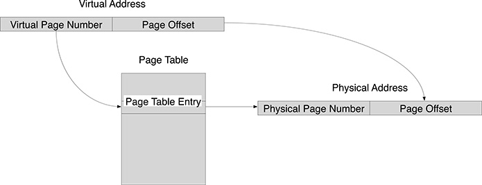
FIGURE 2.5
The Virtual Memory address translation.
Even if virtual memory may seem at a first glance a method merely invented to complicate the engineer’s life, the following example should convince the skeptics of its convenience. Consider two processes running the same program: This is perfectly normal in everyday’s life, and no one is in fact surprised by the fact that two Web browsers or editor programs can be run by different processes in Linux (or tasks in Windows). Recalling that a program is composed of a sequence of machine instructions handling data in processor registers and in memory, if no virtual memory were supported, the two instances of the same program run by two different processes would interfere with each other since they would access the same memory locations (they are running the same program). This situation is elegantly solved, using the virtual memory mechanism, by providing two different mappings to the two processes so that the same virtual address page is mapped onto two different physical pages for the two processes, as shown in Figure 2.6. Recalling that the address translation is driven by the content of the page table, this means that the operating systems, whenever it assigns the processor to one process, will also set accordingly the corresponding page table entries. The page table contents become therefore part of the set of information, called Process Context, which needs to be restored by the operating system in a context switch, that is whenever a process regains the usage of the processor. Chapter 3 will describe process management in more detail; here it suffices to know that virtual address translation is part of the process context.
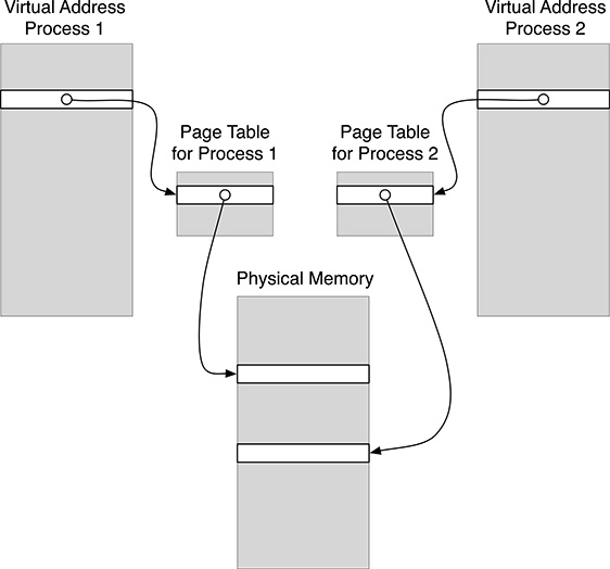
FIGURE 2.6
The usage of virtual address translation to avoid memory conflicts.
Virtual memory support complicates quite a bit the implementation of an operating system, but it greatly simplifies the programmer’s life, which does not need concerns about possible interferences with other programs. At this point, however, the reader may be falsely convinced that in an operating system not supporting virtual memory it is not possible to run the same program in two different processes, or that, in any case, there is always the risk of memory interferences among programs executed by different processes. Luckily, this is not the case, but memory consistence can be obtained only by imposing a set of rules for programs, such as the usage of the stack for keeping local variables. Programs which are compiled by a C compiler normally use the stack to contain local variables (i.e., variables which are declared inside a program block without the static qualifier) and the arguments passed in routine calls. Only static variables (i.e., local variables declared with the static qualifier or variables declared outside program blocks) are allocated outside the stack. A separate stack is then associated with each process, thus allowing memory insulation, even on systems supporting virtual memory. When writing code for systems without virtual memory, it is therefore important to pay attention in the usage of static variables, since these are shared among different processes, as shown in Figure 2.7. This is not necessarily a negative fact, since a proper usage of static data structures may represent an effective way for achieving interprocess communication. Interprocess communication, that is, exchanging data among different processes, can be achieved also with virtual memory, but in this case it is necessary that the operating system is involved so that it can set-up the content of the page table in order to allow the sharing of one or more physical memory pages among different processes, as shown in Figure 2.8.
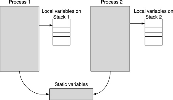
FIGURE 2.7
Sharing data via static variable on systems which do not support Virtual Addresses.
2.3.3 Handling Data Streaming from the Camera Device
Coming back to the acquisition of camera images using double buffering, we face the problem of properly mapping the buffers filled by the driver, running in Kernel mode, and the process running the frame acquisition program, running in User mode. When operating in Kernel mode, Linux uses in fact direct physical addresses (the operating system must have a direct access to every computer resource), so the buffer addresses seen by the driver will be different from the addresses of the same memory areas seen by the program. To cope with such a situation, Linux provides the mmap() system call. In order to understand how mmap() works, it is necessary to recall the file model adopted by Linux to support device I/O programming. In this conceptual model, files are represented by a contiguous space corresponding to the bytes stored in the file on the disk. A current address is defined for every file, representing the index of the current byte into the file. So address 0 refers to the first byte of the file, and address N will refer to the N th byte of the file. Read-and-write operations on files implicitly refer to the current address in the file. When N bytes are read or written, they are read or written starting from the current address, which is then incremented by N. The current address can be changed using the lseek() system routine, taking as argument the new address within the file. When working with files, mmap() routine allows to map a region in the file onto a region in memory. The arguments passed to mmap() will include the relative starting address of the file region and the size in bytes of the region, and mmap() will return the (virtual) start address in memory of the mapped region. Afterwards, reading and writing in that memory area will correspond to reading and writing into the corresponding region in the file. The concept of current file address cannot be exported as it is when using the same abstraction to describe I/O devices. For example, in a network device the current address is meaningless: read operations will return the bytes that have just been received, and write operations will send the passed bytes over the network. The same holds for a video device, and read operation will get the acquired image frame, not read from any “address.” However, when handling memory buffers in double buffering, it is necessary to find some way to map region of memory used by the driver into memory buffers for the program. mmap() can be used for this purpose, and the preparation of the shared buffers is carried out in two steps:
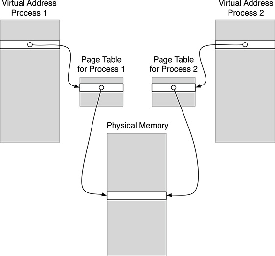
FIGURE 2.8
Using the Page Table translation to map possibly different virtual addresses onto the same physical memory page.
The driver allocates the buffers in its (physical) memory space, and returns (in a data structure passed to
ioctl()) the unique address (in the driver context) of such buffers. The returned addresses may be the same physical address of the buffers, but in any case they are seen outside the driver as addresses referred to the conceptual file model.The user programs calls
mmap()to map such buffers in its virtual memory onto the driver buffers, passing as arguments the file addresses returned in the previousioctl()call. After themmap()call the memory buffers are shared between the driver, using physical addresses, and the program, using virtual addresses.
The code of the program using multiple buffering for handling image frame streaming from the camera device is listed below.
# include <fcntl.h>
# include <stdio.h>
# include <stdlib.h>
# include <string.h>
# include <errno.h>
# include <linux/videodev2.h>
# include <asm/unistd.h>
# include <poll.h>
# define MAX_FORMAT 100
# define FALSE  0
# define TRUE  1
# define CHECK_IOCTL_STATUS(message) \
if(status == -1)                       \
{                                      \
    perror (message);                  \
    exit(EXIT_FAILURE);                \
}
main (int  argc, char * argv [])
{
    int fd, idx,  status ;
    int pixelformat;
    int imageSize;
    int width, height ;
    int yuyvFound;
    struct  v412_capability cap;        //Query Capability structure
    struct  v412_fmtdesc  fmt;          //Query Format Description structure
    struct  v412_format  format ;       //Query Format structure
    struct  v412_requestbuffers reqBuf; //Buffer request structure
    struct  v412_buffer buf;            //Buffer setup structure
    enum  v412_buf_type  bufType ;      //Used to enqueue buffers
    typedef struct   {                  //Buffer descriptors
       void  * start ;
       size_t  length ;
    } bufferDsc;
    int idx;
    fd_set  fds;                        //Select descriptors
    struct timeval   tv;                //Timeout specification structure
/* Step 1: Open the device  */
    fd = open ("/dev/ video1",  O_RDWR);
/* Step 2: Check streaming capability */
    status = ioctl (fd, VIDIOC_QUERYCAP,   &cap);
    CHECK_IOCTL_STATUS(" Error querying capability")
    if (!(cap.capabilities & V4L2_CAP_STREAMING))
    {
       printf ("Streaming NOT supported
");
       exit (EXIT_FAILURE);
    }
/* Step 3: Check supported formats  */
    yuyvFound  = FALSE ;
    for (idx = 0; idx < MAX_FORMAT;  idx ++)
    {
       fmt.index = idx;
       fmt.type = V4L2_BUF_TYPE_VIDEO_CAPTURE;
       status = ioctl (fd, VIDIOC_ENUM_FMT,   &fmt);
       if (status != 0) break ;
       if (fmt.pixelformat ==    V4L2_PIX_FMT_YUYV)
       {
          yuyvFound = TRUE;
          break ;
       }
    }
    if (! yuyvFound)
    {
       printf (" YUYV format not supported
");
       exit (EXIT_FAILURE);
    }
/* Step 4: Read current format definition  */
    memset (&format, 0, sizeof (format));
    format.type  =  V4L2_BUF_TYPE_VIDEO_CAPTURE;
    status = ioctl (fd, VIDIOC_G_FMT,  &format);
    CHECK_IOCTL_STATUS(" Error Querying Format ")
/* Step 5: Set format fields to desired values : YUYV coding,
    480 lines, 640 pixels per    line  */
    format.fmt.pix.width = 640;
    format.fmt.pix.height = 480;
    format.fmt.pix.pixelformat = V4L2_PIX_FMT_YUYV;
/* Step 6: Write desired format and check actual image size  */
    status = ioctl (fd, VIDIOC_S_FMT,  &format);
    CHECK_IOCTL_STATUS(" Error Setting Format ");
    width = format.fmt.pix.width ;                   //Image  Width
    height = format.fmt.pix.height ;                 //Image Height
    //Total image size in bytes
    imageSize = (unsigned int) format.fmt.pix.sizeimage;
/* Step 7: request for allocation of 4 frame buffers by the driver  */
    reqBuf.count = 4;
    reqBuf.type  =  V4L2_BUF_TYPE_VIDEO_CAPTURE;
    reqBuf.memory =  V4L2_MEMORY_MMAP;
    status = ioctl (fd, VIDIOC_REQBUFS,  &reqBuf);
    CHECK_IOCTL_STATUS("Error  requesting  buffers ")
/* Check the number of returned buffers.It must be at least 2 */
    if(reqBuf.count <  2)
    {
        printf (" Insufficient buffers
");
        exit (EXIT_FAILURE);
    }
/*  Step 8: Allocate a descriptor for each buffer and request its
     address to the driver. The start address in user space and the
     size of the buffers are recorded in the buffers descriptors. */
    buffers = calloc (reqBuf.  count, sizeof (bufferDsc));
    for(idx = 0; idx < reqBuf.count ;  idx ++)
    {
        buf.type =  V4L2_BUF_TYPE_VIDEO_CAPTURE;
        buf.memory  =  V4L2_MEMORY_MMAP;
        buf.index = idx;
/*  Get the start address in the driver space of buffer idx  */
        status = ioctl (fd, VIDIOC_QUERYBUF,  &buf);
        CHECK_IOCTL_STATUS(" Error querying buffers ")
/*  Prepare the buffer descriptor with the address in user space
     returned by mmap()  */
        buffers [idx ].length = buf.length ;
        buffers [idx ].start = mmap (NULL, buf.length ,
            PROT_READ | PROT_WRITE, MAP_SHARED ,
            fd, buf.m.offset);
        if (buffers [idx].start == MAP_FAILED)
        {
            perror (" Error mapping memory ");
            exit (EXIT_FAILURE);
        }
    }
/*  Step 9: request the driver to enqueue all the buffers
     in a circular list  */
    for(idx = 0; idx < reqBuf.count; idx ++)
    {
        buf.type = V4L2_BUF_TYPE_VIDEO_CAPTURE;
        buf.memory  =  V4L2_MEMORY_MMAP;
        buf.index = idx;
        status = ioctl (fd, VIDIOC_QBUF, &buf);
        CHECK_IOCTL_STATUS("Error enqueuing buffers")
    }
/*  Step 10: start streaming  */
    bufType =  V4L2_BUF_TYPE_VIDEO_CAPTURE;
    status = ioctl (fd, VIDIOC_STREAMON,  &bufType);
    CHECK_IOCTL_STATUS("Error starting streaming")
/*  Step 11: wait for a buffer ready  */
    FD_ZERO (&fds);
    FD_SET (fd, &fds);
    tv.tv_sec =   20;
    tv.tv_usec =   0;
    for (;;)
    {
        status = select (1, &fds, NULL, NULL,   &tv);
        if (status == -1)
        {
            perror (" Error in Select ");
            exit (EXIT_FAILURE);
        }
/*  Step 12: Dequeue buffer  */
        buf.type =  V4L2_BUF_TYPE_VIDEO_CAPTURE;
        buf.memory =  V4L2_MEMORY_MMAP;
        status = ioctl (fd, VIDIOC_DQBUF, &buf);
        CHECK_IOCTL_STATUS(" Error dequeuing buffer ")
/*  Step 13: Do image processing  */
        processImage(buffers [ buf.index ].start, width, height,  imagesize);
/*  Step 14: Enqueue used buffer  */
       status = ioctl (fd, VIDIOC_QBUF, &buf);
       CHECK_IOCTL_STATUS(" Error  enqueuing  buffer ")
    }
}
Steps 1–6 are the same of the previous program, except for step 2, where the streaming capability of the device is now checked. In Step 7, the driver is asked to allocate four image buffers. The actual number of allocated buffers is returned in the count field of the v412_requestbuffers structure passed to ioctl(). At least two buffers must have been allocated by the driver to allow double buffering. In Step 8 the descriptors of the buffers are allocated via the calloc() system routine (every descriptor contains the dimension and a pointer to the associated buffer). The actual buffers, which have been allocated by the driver, are queried in order to get their address in the driver’s space. Such an address, returned in field m.offset of the v412_buffer structure passed to ioctl(), cannot be used directly in the program since it refers to a different address space. The actual address in the user address space is returned by the following mmap() call. When the program arrives at Step 9, the buffers have been allocated by the driver and also mapped to the program address space. They are now enqueued by the driver, which maintains a linked queue of available buffers. Initially, all the buffers are available: every time the driver has acquired a frame, the first available buffer in the queue is filled. Streaming, that is, frame acquisition, is started at Step 10, and then at Step 11 the program waits for the availability of a filled buffer, using the select() system call. Whenever select() returns, at least one buffer contains an acquired frame. It is dequeued in Step 12, and then enqueued in Step 13, after it has been used in image processing. The reason for dequeuing and then enqueuing the buffer again is to make sure that the buffer will not be used by the driver during image processing.
Finally, image processing will be carried out by routine processImage(), which will first build a byte buffer containing only the luminance, that is, taking the first byte of every 16 bit word of the passed buffer, coded using the YUYV format.
2.4 Edge Detection
In the following text we shall proceed with the case study by detecting, for each acquired frame, the center of a circular shape in the acquired image. In general, image elaboration is not an easy task, and its results may not only depend on the actual shapes captured in the image, but also on several other factors, such as illumination and angle of view, which may alter the information retrieved from the image frame. Center coordinates detection will be performed here in two steps. Firstly, the edges in the acquired image are detected. This first step allows reducing the size of the problem, since for the following analysis it suffices to take into account the pixels representing the edges in the image. Edge detection is carried out by computing the approximation of the gradients in the X (Lx) and Y (Ly) directions for every pixel of the image, selecting, then, only those pixels for which the gradient magnitude, computed as , is above a given threshold. In fact, informally stated, an edge corresponds to a region where the brightness of the image changes sharply, the gradient magnitude being an indication of the “sharpness” of the change. Observe that in edge detection we are only interested in the luminance, so in the YUYV pixel format, only the first byte of every two will be considered. The gradient is computed using a convolution matrix filter. Image filters based on convolution matrix filters are very common in image elaboration and, based on the matrix used for the computation, often called kernel, can perform several types of image processing. Such a matrix is normally a 3 x 3 or 5 x 5 square matrix, and the computation is carried out by considering, for each pixel image P (x, y), the pixels surrounding the considered one and multiplying them for the corresponding coefficient of the kernel matrix K. Here we shall use a 3 x 3 kernel matrix, and therefore the computation of the filtered pixel value Pf (x, y) is
Here, we use the Sobel Filter for edge detection, which defines the following two kernel matrixes:
for the gradient along the X direction, and
for the gradient along the Y direction.
The C source code for the gradient detection is listed below:
# define  THRESHOLD  100
/* Sobel matrixes  */
static int GX [3][3];
static int GY [3][3];
/* Initialization of the Sobel matrixes, to be called before
Sobel filter  computation */
static void initG ()
{
/*  3x3 GX Sobel mask.  */
    GX [0][0] = -1; GX [0][1] = 0; GX [0][2] = 1;
    GX [1][0] = -2; GX [1][1] = 0; GX [1][2] = 2;
    GX [2][0] = -1; GX [2][1] = 0; GX [2][2] = 1;
/*  3x3 GY Sobel mask.  */
    GY [0][0] =  1; GY [0][1] =  2; GY [0][2] =  1;
    GY [1][0] =  0; GY [1][1] =  0; GY [1][2] =  0;
    GY [2][0] = -1; GY [2][1] = -2; GY [2][2] = -1;
}
/* Sobel Filter computation for Edge detection.  */
static void  makeBorder(char *  image,  char * border,  int cols,  int rows)
/* Input image is passed in the byte array image (cols x rows pixels)
     Filtered image is returned in byte array border */
{
    int x, y, i, j, sumX, sumY,   sum;
    for(y = 0; y <= (rows -1); y++)
    {
       for(x = 0; x <= (cols -1); x++)
       {
          sumX = 0;
          sumY = 0;
/* handle image boundaries */
          if(y == 0 || y ==   rows -1)
             sum =  0;
          else if(x == 0 || x   ==  cols -1)
             sum =  0;
/* Convolution starts here */
             else
             {
/*  X Gradient  */
             for(i = -1; i <= 1;    i++)
             {
                 for(j =- 1; j <= 1;   j ++)
                 {
                     sumX = sumX + (int)((*(image + x + i  +
                       (y + j)* cols)) * GX[i + 1][j + 1]);
                 }
             }
/*  Y Gradient  */
             for(i = -1; i <= 1;    i++)
             {
                for(j = -1; j <= 1;   j ++)
                {
                    sumY = sumY + (int)((*(image   + x + i  +
                        (y + j)* cols)) * GY[i + 1][j + 1]);
                }
             }
/* Gradient Magnitude approximation to avoid square root operations  */
             sum = abs(sumX) +  abs(sumY);
          }
           if(sum > 255) sum = 255;
           if(sum < THRESHOLD) sum = 0;
          *(border  + x + y* cols) = 255 - (unsigned char)(sum);
       }
    }
}
Routine makeBorder() computes a new image representing the edges of the scene in the image. Only such pixels will then be considered in the following computation for detecting the center of a circular shape in the image.
2.4.1 Optimizing the Code
Before proceeding, it is worth to consider the performance of such algorithm. In fact, if we intend to use the edge detection algorithm in an embedded system with realtime constraints, we must ensure that its execution time will be bound to a given value, short enough to guarantee that the system will meet its requirements. First of all we observe that for every pixel of the image, 2*3*3 multiplications and sums are performed to compute the X and Y gradients, not considering the operation on the matrix indices. This means that, supposing a square image of size N is considered, the number of operation is proportional to N*N, and we say that the algorithm has complexity O(N2). This notation is called the big-O notation and provides an indication of the complexity for computer algorithms. More formally, given two functions f (x) and g(x), if a value M and a value x0 exist for which the following condition holds:
for every x > x0, then we say that f (x) is O(g(x)).
Informally stated, the above notation states that, for very large values of x the two functions tend to become proportional. For example, if f (x) = 3x and g(x) = 100x + 1000, then we can find a pair M, x0 for which 2.4 holds, and therefore f (x) is O(g(x)). However, if we consider f (x) = 3x2 instead, it is not possible to find such a pair M, x0. In fact, f (x) grows faster than every multiple of g(x). Normally, when expressing the complexity of an algorithm, the variable x used above represents the “dimension” of the problem. For example, in a sorting algorithm, the dimension of the problem is represented by the dimension of the vector to be sorted. Often some simplifying assumption must be done in order to provide a measure of the dimension to be used in the big-O notation. In our edge detection problem, we make the simplifying assumption that the image is represented by a square pixel matrix of size N, and therefore we can state that the Sobel filter computation is O(N2) since the number of operations is proportional to N2.
The big-O notation provides a very important measurement of the efficiency for computer algorithms, which normally become unmanageable when the dimension of the problem increases. Take as an example the algorithms for sorting a given array of values. Elementary sorting algorithms such as Bubble Sort or Insertion Sort require a number of operation that is proportional to N2, where N is the dimension of the array to be sorted and therefore are O(N2). Other sorting algorithms, such as Shell Sort and Quick Sort are instead O(Nlog(N)). This implies that for very large arrays, only the latter algorithms can be used in practice because the number of operations becomes orders of magnitude lower in this case.
Even if the big-O notation is very important in the classification of algorithms and in determining their applicability when the dimension of the problem grows, it does not suffice for providing a complete estimate of the computation time. To convince ourselves of this fact, it suffices to consider two algorithms for a problem of dimension N, the first one requiring f (N) operations, and the second one requiring exactly 100f (N). Of course, we would never choose the second one; however they are equivalent in the big-O notation, being both O(f (N)).
Therefore, in order to assess the complexity of a given algorithm and to optimize it, other techniques must be considered, in addition to the choice of the appropriate algorithm. This the case of our application: given the algorithm, we want to make its computation as fast as possible.
First of all, we need to perform a measurement of the time the algorithm takes. A crude but effective method is to use the system routines for getting the current time, and measure the difference between the time measured first and after the computation of the algorithm. The following code snippet makes a raw estimation of the time procedure makeBorder() takes in a Linux system.
# define  ITERATIONS  1000
struct time_t  beforeTime,  afterTime;
int  executionTime;
....
gettimeofday(&beforeTime, NULL);
for(i = 0; i < ITERATIONS;   i ++)
    makeBorder(image,  border, cols, rows);
gettimeofday(&afterTime,  NULL);
/*  Execution time is expressed in microseconds  */
executionTime = (afterTime. tv_sec  -  beforeTime. tv_sec) * 1000000
    + afterTime. tv_usec  -  beforeTime. tv_usec ;
executionTime /= ITERATIONS;
...
The POSIX routine gettimeofday() reads the current time from the CPU clock and stores it in a time_t structure whose fields define the number of seconds (tv_sec) and microseconds (tv_usec) from the Epoch, that is, a reference time which, for POSIX, is assumed to be 00:00:00 UTC, January 1, 1970.
The execution time measured in this way can be affected by several factors, among which can be the current load of the computer. In fact, the process running the program may be interrupted during execution by other processes in the system. Even after setting the priority of the current process as the highest one, the CPU will be interrupted many times for performing I/O and for the operating system operation. Nevertheless, if the computer is not loaded, and the process running the program has a high priority, the measurement is accurate enough.
We are now ready to start the optimization of our edge detection algorithm. The first action is the simplest one: let the compiler do it. Modern compilers perform very sophisticated optimization of the machine code that is produced when parsing the source code. It is easy to get an idea of the degree of optimization by comparing the execution time when compiling the program without optimization (compiler flag -O0) and with the highest degree of optimization (compiler flag -O3), which turns out to be 5–10 times shorter for the edge detection routine. The optimization performed by the compiler addresses the following aspects:
Code Reduction: Reducing the number of machine instructions makes the program execution faster. Very often in programs the same information is computed many times in different parts. So the compiler can reuse the value computed before, instead of executing again a sequence of machine instructions leading to the same result. The compiler tries also to carry out computation in advance, rather than producing the machine instructions for doing it. For example, if an expression formed by constant values is present in the source code, the compiler can produce the result at compile time, rather than doing it during the program execution. The compiler also moves away from loops the computation that does not depend on loop variable, and which therefore would produce the same result at every loop iteration.
Observe that code reduction does not mean reduction in the size of the produced program; rather, it reduces the number of instruction actually executed during the program. For example, whenever the number N of loop iterations can be deduced at compile time (i.e., does not depend on run-time information) and N is not too high, compilers often replace the conditional jump instruction by concatenating N segments of machine instruction, each corresponding to the loop body. The resulting executable program is longer, but the number of instructions actually performed is lower since the conditional jumps instruction and the corresponding condition evaluation are avoided. For the same reason, compilers can also perform inline expansion when a routine is called in the program. Inserting the code of the routine again makes the size of the executable program bigger, but avoids the overhead due to the routine invocation and the passage of the arguments.
Instruction Selection: Even if several operations defined in the source code, such as multiplications, can be directly executed by machine instruction, this choice does not represent the most efficient one. Consider, for example, a multiplication by two: this can be performed either with a multiplication (MUL) or with an addition (ADD) machine instruction. Clearly, the second choice is preferable since in most computer architectures addition is performed faster than multiplication. Therefore, the compiler selects the most appropriate sequence of machine instructions for carrying out the required computation. Observe that again this may lead to the generation of a program with a larger number of machine instructions, where some operations for which a direct machine instruction exists are instead implemented with a longer sequence of faster machine instruction. In this context, a very important optimization carried out by the compiler is the recognition of induction variables in loops and the replacement of operations on such variables with simpler ones. As an example, consider the following loop:
for (i = 0; i < 10; i++)
{
    a = 15 * i;
    .....
}
Variable
iis an induction variable, that is, a variable which gets increased or decreased by a fixed amount on every iteration of a loop, or which is a linear function of another induction variable. In this case, it is possible to replace the multiplication with an addition, getting the equivalent loop:a = 0; for (i = 0; i < 10; i++) { a = a + 15; ..... }The compiler recognizes, then, induction variables and replaces more complex operations with additions. This optimization is particularly useful for the loop variables used as indexes in arrays; in fact, many computer architectures define memory access operations (arrays are stored in memory and are therefore accessed via memory access machine instructions such as LOAD or STORE), which increment the passed memory index by a given amount in the same memory access operation.
Register Allocation: Every computer architecture defines a number of registers that can store temporary information during computation. Registers are implemented within the processor, and therefore reading or writing to a register is much faster than reading and writing from memory. For this reason the compiler will try to use processor registers as far as possible, for example, using registers to hold the variables defined in the program. The number of registers is, however, finite (up to some tents), and therefore it is not possible to store all the variables into registers. Memory locations must be used, too. Moreover, when arrays are used in the program, they are stored in memory, and access to array elements in the program normally requires an access to memory in run time. The compiler uses a variety of algorithms to optimize the use of registers, and to maximize the likelihood that a variable access will be performed by a register access. For example, if a variable stored in memory is accessed for the second time, and it has not been changed since its first access (something which can be detected under certain conditions by the compiler), then the compiler will temporarily hold a copy of the variable on a register so that the second time it is read from the register instead from memory.
Machine-Dependent Optimization: the above optimizations hold for every computer. In fact, reducing the number and the complexity of instructions executed in run time will always reduce execution time, as well as optimizing the usage of registers. There are, however, other optimizations that depend on specific computer architecture. A first set of optimizations addresses the pipeline. All modern processors are pipelined, that is the execution of machine instructions is implemented as a sequence of stages. Each stage is carried out by a different processors components. For example, a processor may define the following stages for a machine instruction:
Fetch: read the instruction from memory;
Decode: decode the machine instruction;
Read arguments: load the arguments of the machine instruction (from registers or from memory);
Execute: do what the instruction specifies;
Store results: store the results of the execution (to registers or to memory).
A separate hardware processor component, called the pipeline stage, will carry out every stage. So, when the first stage has terminated fetching the instruction N, it can start fetching instruction N + 1 while instruction N is being decoded. After a startup time, under ideal conditions, the K stages of the pipeline will all be busy, and the processor is executing K instruction in parallel, reducing the average execution time of a factor of K. There are, however, several conditions that may block the parallel execution of the pipeline stages, forcing a stage to wait for some clock cycle before resuming operation. One such condition is given by the occurrence of two consecutive instructions, say, instructions N and N + 1 in the program, where the latter uses as input the results of the former. In this case, when instruction N + 1 enters its third stage (Read arguments), instructions N enters the execute phase. However, instruction N + 1 cannot proceed in reading the arguments, since they have not yet been reported by the previous instruction. Only when instruction N finishes its execution (and its results have been stored) execution N + 1 can resume its execution, thus producing a delay in the execution of two clock cycles, assuming that every pipeline stage is executed in one clock period. This condition is called Data Hazard and depends on the existence of sequences of two or more dependent consecutive instructions.
If the two instruction were separated by at least two independent instructions in the program sequence, no data hazard would occur and no time would be spent with the pipeline execution partially blocked. The compiler, therefore, tries to separate dependent instruction in the program. Of course, instructions cannot be freely moved in the code, and code analysis is required to figure out which instruction sequence rearrangement are legal, that is, which combination maintain the program correct. This kind of analysis is also performed by the compiler to take advantage of the availability of multiple execution units in superscalar processors. In fact, instructions can be executed in parallel only when they are independent from each other.
At this point we may be tempted to state that the all the possible optimizations in the edge detection program have been carried out by the compiler, and there is no need to further analyze the program for reducing its execution time. This is, however, not completely true: while compilers are very clever in optimizing code, very often achieving a better optimization than what can be achieved with manual optimization, there is one aspect of the program in which compilers cannot exploit extreme optimization—that is, memory access via pointers. We have already seen that a compiler can often maintain in a register a copy of a variable stored in memory so that the register copy can be used instead. However, it is not possible to store in a register a memory location accessed via a pointer and reuse it afterwards in spite of the memory location, because it is not possible to make sure that the memory address has not been modified in the meantime. In fact, while in many cases the compiler can analyze in advance how variables are used in the program, in general it cannot do the same for memory location accessed via pointers because the pointer values, that is, the memory addresses, are normally computed run time, and cannot therefore be foreseen during program compilation.
As we shall see shortly, there is still room for optimization in the edge detection routine, but it is necessary to introduce first some concepts of memory caching.
In order to speed memory accesses computers use memory caches. A memory cache is basically a fast memory that is much faster that the RAM memory used by the processor, and which holds data recently accessed by the computer. The memory cache does not correspond to any fixed address in the addressing space of the processor, and therefore contains only copies for memory locations stored in the RAM. The caching mechanism is based on a common fact in programs: locality in memory access. Informally stated, memory access locality expresses the fact that if a processor makes a memory access, say, at address K, the next access in memory is likely to occur at an address that is close to K. To convince ourselves of this fact, consider the two main categories of memory data access in a program execution: fetching program instructions and accessing program data. Fetching memory instructions (recall that a processor has to read the instruction from memory in order to execute it) is clearly sequential in most cases. The only exception is for the Jump instructions, which, however, represent a small fraction of the program instructions. Data is mostly accessed in memory when the program accesses array elements, and arrays are normally (albeit not always) accessed in loops using some sort of sequential indexing.
Cache memory is organized in blocks (called also cache lines), which can be up to a few hundreds bytes large. When the processor tries to access a memory location for reading or writing a data item at a given address, the cache controller will first check if a cache block containing that location is currently present in the cache. If it is found in the cache memory, fast read/write access is performed in the cached copy of the data item. Otherwise, a free block in the cache is found (possibly copying in memory an existing cache block if the cache is full), and a block of data located around that memory address is first copied from memory to the cache. The two cases are called Cache Hit and Cache Miss, respectively. Clearly, a cache miss incurs in a penalty in execution time (the copy of a block from memory to cache), but, due to memory access locality, it is likely that further memory accesses will hit the cache, with a significant reduction in data access time.
The gain in performance due to the cache memory depends on the program itself: the more local is memory access, the faster will be program execution. Consider the following code snippet, which computes the sum of the elements of a MxN matrix.
double  a[M][N];
double sum =  0;
for(i = 0; i < M, i ++)
    for(j = 0; j < N; j ++)
        sum += a[i][j];
In C, matrixes are stored in row first order, that is, rows are stored sequentially. In this case a[i][j] will be adjacent in memory to a[i][j+1], and the program will access matrix memory sequentially. The following code is also correct, differing from the previous one only for the exchange of the two for statements.
double  a[M][N];
double sum =  0;
for(j = 0; j < N; j ++)
    for(i = 0; i < M, i ++)
        sum += a[i][j];
However in this case memory access is not sequential since matrix elements a[i][j] and a[i+1][j] are stored in memory locations that are N elements far away. In this case, the number of cache misses will be much higher than in the former case, especially for large matrixes, affecting the execution time of that code.
Coming back to routine makeBorder(), we observe that it is accessing memory in the right order. In fact, what the routine basically does is to consider a 3 x 3 matrix sweeping along the 480 rows of the image. The order of access is therefore row first, corresponding to the order in which bytes are stored in the image buffer. So, if bytes are being considered in a “cache friendly” order, what can we do to improve performance? Recall that the compiler is very clever in optimizing access to information stored in program variables, but is mostly blind as regard the management of information stored in memory (i.e., in arrays and matrixes). This fact suggests to us a possible strategy: move the current 3 x 3 portion of the image being considered in the Sobel filter into 9 variables. Filling this set of 9 variables the first time a line is considered will require reading 9 values from memory, but at the following iterations, that is, moving the 3 x 3 matrix one position left, only three new values will be read from memory, the others already being stored in program variables. Moreover, the nine multiplications and summations required to compute the value of the current output filter can be directly expressed in the code, without defining the 3 x 3 matrixes GX and GY used in the program listed above. The new implementation of makeBorder() is listed below, using the new variables c11, c12, ..., c33 to store the current portion of the image being considered for every image pixel.
void  makeBorder(char   *image, char *border,   int  cols, int  rows)
{
    int x, y, sumX, sumY, sum;
/* Variables to hold the 3x3 portion of the image used in the computation
of the Sobel filter output  */
    int  c11 ,c12 ,c13 ,c21 ,c22 ,c23 ,c31 ,c32, c33;
    for(y = 0; y <= (rows -1); y++)
    {
    /* First image row: the first row of cij is zero */
       if (y == 0)
       {
            c11 = c12 = c13 = 0;
       }
       else
    /* First image column: the first column of cij matrix is zero  */
       {
            c11 =0;
            c12 = *(image + (y - 1) *  cols);
            c13 = *(image + 1 + (y - 1)* cols);
       }
       c21 = 0;
       c22 = *(image +  y* cols);
       c23 = *(image + 1 + y*  cols);
       if (y == rows - 1)
    /* Last image row: the third row of cij matrix is zero  */
       {
            c31 = c32 = c33 =  0;
       }
       else
       {
            c31 =0;
            c32 = *(image + (y + 1)* cols);
            c33 = *(image + 1 + (y + 1)* cols);
       }
/*  The 3x3 matrix corresponding to the first pixel of the current image
     row has been loaded in program variables .
     The following iterations will only  load
     from memory the rightmost column of such matrix  */
       for(x = 0; x <= (cols -1);  x++)
       {
            sumX = sumY =    0;
/* Skip image boundaries */
            if(y == 0 || y == rows -1)
                sum =  0;
            else if(x == 0 || x ==  cols -1)
                sum =  0;
/* Convolution starts here.
     GX and GY parameters are now “cabled” in the code */
            else
            {
                 sumX = sumX -    c11;
                 sumY = sumY +    c11;
                 sumY = sumY +    2* c12;
                 sumX = sumX +    c13;
                 sumY = sumY +    c13;
                 sumX = sumX - 2 *    c21;
                 sumX = sumX +    2* c23;
                 sumX = sumX -    c31;
                 sumY = sumY -    c31;
                 sumY = sumY -  2* c32;
                 sumX = sumX +  c33;
                 sumY = sumY -  c33;
                 if(sumX < 0) sumX =  -sumX; //Abs value
                 if(sumY < 0) sumY =  -sumY;
                 sum = sumX +  sumY ;
            }
/*  Move one pixel on the right in the current row .
    Update the first / last row only if not in the first / last image row  */
            if(y > 0)
            {
                 c11 =  c12;
                 c12 =  c13;
                 c13 =  *(image + x + 2 + (y - 1)  * cols);
            }
            c21 =  c22;
            c22 =  c23;
            c33 = *(image + x +2 + y * cols);
            if(y < cols - 1)
            {
                 c31 =  c32;
                 c32 =  c33;
                 c33 =  *(image + x + 2 + (y + 1)  * cols);
            }
            if(sum > 255) sum =  255;
            if(sum < THRESHOLD) sum =0;
/*  Report the new pixel in the output image  */
            *(border  + x + y* cols) = 255 - (unsigned char)(sum);
      }
    }
}
The resulting code is for sure less readable then the previous version, but, when compiled, it produces a code that is around three times faster because the compiler has now more chance for optimizing the management of information, being memory access limited to the essential cases.
In general code optimization is not a trivial task and requires ingenuity and a good knowledge of the optimization strategies carried out by the compiler. Very often, in fact, the programmer experiences the frustration of getting no advantage after working hard in optimizing his/her code, simply because the foreseen optimization had already been carried out by the compiler. Since optimized source code is often much less readable that a nonoptimized one, implementing a given algorithm taking care also of possible code optimization, may be an error-prone task. For this reason, implementation should be done in two steps:
Provide a first implementation with no regard to efficiency, but concentrating on a clearly readable and understandable implementation. At this level, the program should be fully debugged to make sure that no errors are present in the code, preparing also a set of test cases that fully covers the different aspects of the algorithm.
Starting from the previous implementation, and using the test cases prepared in the first step, perform optimization, possibly in steps, in order to address separately possible sources of inefficiency. At every try (not all the tentatives will actually produce a faster version) check the correctness of the new code and the amount of gained performance.
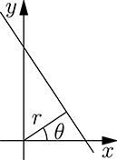
FIGURE 2.9
r and θ representation of a line.
2.5 Finding the Center Coordinates of a Circular Shape
After the edge detection stage, a much reduced number of pixels has to be taken into consideration to compute the final result of image analysis in our case study: locating the coordinates of the center of a circular shape in the image. To this purpose, the Hough transform will be used, a technique for feature extraction in images. In the original image, every element of the image matrix brings information on the luminance of the corresponding pixel (we are not considering colors here). The Hough transform procedure converts pixel luminance information into a set of parameters, so that a voting procedure can be defined in the parameter space to derive the desired feature, even in the case of imperfect instances of objects in the input image.
The Hough transform was originally used to detect lines in images. In this case, the parameter space components are r and θ, where every line in the original image ir represented by a (r, θ) pair, as shown in Figure 2.9. Using parameters r and θ, the equation of a line in the x, y plane is expressed as:
Imagine an image containing one line. After edge detection, the pixels associated with the detected edges may belong to the line, or to some other element of the scene represented by the image. Every such pixel at coordinates (x0, y0) is assumed by the algorithm as belonging to a potential line, and the (infinite) set of lines passing for (x0, y0) is considered. For all such lines, the associated parameters r and θ obey to the following relation:
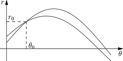
FIGURE 2.10
(r, θ) relationship for points (x0, y0) and (x1, y1).
that is, a sinusoidal law in the plane (r, θ). Suppose now that the considered pixel effectively belongs to the line, and consider another pixel at position (x1, y1), belonging to the same line. Again, for the set of lines passing through (x1, y1), their r and θ will obey the law:
Plotting (2.5) and (2.7) in the (r, θ) (Figure 2.10) we observe that the two graphs intersect in (r0, θ0), where r0 and θ0 are the parameters of the line passing through (x0, y0) and (x1, y1). Considering every pixel on that line, all the corresponding curves in place (r, θ) will intersect in (r0, θ0). This suggests a voting procedure for detecting the lines in an image. We must consider, in fact, that in an image spurious pixels are present, in addition to those representing the line. Moreover, the (x, y) position of the line pixels may lie not exactly in the expected coordinates for that line. So, a matrix corresponding to the (r, θ) plane, initially set to 0, is maintained in memory. For every edge pixel, the matrix elements corresponding to all the pairs (r, θ) defined by the associated sinusoidal relation are incremented by one. When all the edge pixels have been considered, supposing a single line is represented in the image, the matrix element at coordinates (r0, θ0) will hold the highest value, and therefore it suffices to choose the matrix element with the highest value, whose coordinates will identify the recognized line in the image.
A similar procedure can be used to detect the center of a circular shape in the image. Assume initially that the radius R of such circle is known. In this case, a matrix with the same dimension of the image is maintained, initially set to 0. For every edge pixel (x0, y0) in the image, the circle of radius R centered in (x0, y0) is considered, and the corresponding elements in the matrix incremented by 1. All such circles intersect in the center of the circle in the image, as shown in Figure 2.11. Again, a voting procedure will allow discovery of the center of the circle in edge image, even in presence of spurious pixels, and the approximate position of the pixels representing the circle edges. If the radius R is not known in advance, it is necessary to repeat the above procedure for different values of R and choose the radius value that yields the maximum count value for the candidate center. Intuitively, this holds, because only when the considered radius is the right one will all the circles built around the border pixels of the original circle intersect in a single point.
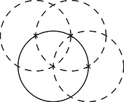
FIGURE 2.11
Circles drawn around points over the circumference intersect in the circle center.
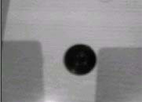
FIGURE 2.12
A sample image with a circular shape.
Observe that even if the effective radius of the circular object to be detected in the image is known in advance, the radius of its shape in the image may depend on several factors, such as its distance from the camera, or even from the illumination of the scene, which may yield slightly different edges in the image, so in practice it is always necessary to consider a range of possible radius values.
The overall detection procedure is summarized in Figures 2.12, 2.13, 2.14, and 2.15. The original image and the detected edges are shown in Figures 2.12 and 2.13, respectively. Figure 2.14 is a representation of the support matrix used in the detection procedure. It can be seen that most of the circles in the image intersect in a single point (the others are circles drawn around the other edges of the image), reported then in the original image in Figure 2.15.
The code of routine findCenter() is listed below. Its input arguments are the radius of the circle, the buffer containing the edges of the original image (created by routine makeBorder()), and the number of rows and columns. The routine returns the position of the detected center and a quality indicator, expressed as the normalized maximum value in the matrix used for center detection. The buffer for such a matrix is passed in the last argument.
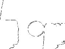
FIGURE 2.13
The image of 2.12 after edge detection.
FIGURE 2.14
The content of the voting matrix generated from the edge pixels of 2.13.
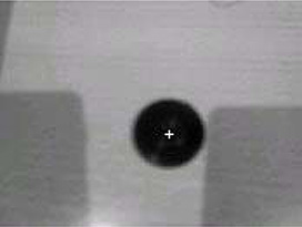
FIGURE 2.15
The detected center in the original image.
/*  Black threshold :
     a pixel value less than the threshold is considered black.  */
# define BLACK_LIMIT 10
void  findCenter(int  radius, unsigned char *buf, int  rows, int cols ,
    int * retX, int *retY, int *retMax, unsigned char *map)
{
    int x, y, l, m, currCol, currRow, maxCount =           0;
    int maxI   = 0, maxJ = 0;
/*  Square roots needed for computation are computed only once
     and maintained in array sqr  */
    static int sqr [2  *  MAX_RADIUS];
    static int  sqrInitialized = 0;
/*  Hit counter, used to normalize the returned quality indicator  */
    double  totCounts =   0;
/*  The matrix is initially set to 0 */
    memset (map, 0, rows * cols);
/*  If square root values not yet initialized, compute them  */
    if (! sqrInitialized)
    {
        sqrInitialized = 1;
        for(l = -radius ; l <= radius ;  l ++)
/*integer approximation of sqrt (radius^2 – l ^2)  */
            sqr[l+ radius ] = sqrt (radius * radius - l*l) + 0.5;
    }
    for(currRow = 0; currRow < rows ;  currRow ++)
    {
        for(currCol = 0; currCol < cols; currCol ++)
        {
/*  Consider only pixels corresponding to borders of the image
     Such pixels are set by makeBorder as dark ones*/
            if(buf[currRow * cols + currCol] <= BLACK_LIMIT)
            {
               x =   currCol ;
               y =   currRow ;
/*  Increment the value of the pixels in map buffer which corresponds to
     a circle of the given radius centered in (currCol, currRow)  */
               for(l = x - radius ; l <= x+ radius ; l++)
               {
                   if(l < 0 || l >=  cols)
                      continue ;  // Out of image X range
                   m = sqr[l-x+ radius ];
                   if(y-m < 0 || y+m >= rows)
                      continue ;  // Out of image Y range
                   map[(y-m)* cols +  l ]++;
                   map[(y+m)* cols +  l ]++;
                   totCounts += 2;     //Two more pixels incremented
/*  Update current maximum  */
                   if(maxCount < map [(y+m)* cols + l])
                   {
                      maxCount = map [(y+m)* cols + l];
                      maxI = y + m;
                      maxJ = l;
                   }
                   if(maxCount < map [(y-m)* cols + l])
                   {
                      maxCount = map [(y-m)* cols + l];
                      maxI = y - m;
                      maxJ = l;
                   }
               }
            }
        }
    }
/*  Return the (X, y) position in the map which yields the largest value  */
    * retX = maxJ ;
    * retY = maxI ;
/*  The returned quality indicator is expressed as maximum pixel
     value in map matrix  */
       * retMax = maxCount ;
}
As stated before, due to small variations of the actual radius of the circular shape in the image, routine findCenter() will be iterated for a set of radius values, ranging between a given minimum and maximum value.
When considering the possible optimization of the detection procedure, we observe that every time routine findCenter() is called, it is necessary to compute the square root values that are required to select the map elements which lie on a circumference centered on the current point. Since the routine is called for a fixed range of radius values, we may think of removing the square root calculation at the beginning of the routine, and to pass on an array of precomputed values, which are prepared in an initialization phase for all the considered radius values. This improvement would, however, bring very little improvement in speed: in fact, only few tens of square root computations (i.e., the pixel dimension of the radius) are carried out every time findCenter() is called, a very small number of operations if compared with the total number of operations actually performed. A much larger improvement can be obtained by observing that it is possible to execute findCenter() for the different radius values in parallel instead of in a sequence. The following code uses POSIX threads, described in detail in Chapter 7, to launch a set of thread, each computing the center coordinates for a given value of the radius. Every thread can be considered an independent flow of execution for the passed routine. In a multicore processor, threads can run on different cores, thus providing a drastic reduction of the execution time because code is executed effectively in parallel. A new thread is created by POSIX routine pthread_create(), which takes as arguments the routine to be executed and the (single) parameter to be passed. As findCenter() accepts multiple input and output parameters, it cannot be passed directly as argument to pthread_create(). The normal practice is to allocate a data structure containing the routine-specific parameters and to pass its pointer to pthread_create() using a support routine (doCenter() in the code below).
After launching the threads, it is necessary to wait for their termination before selecting the best result. This is achieved using POSIX routine pthread_join(), which suspends the execution of the calling program until the specified thread terminates, called in a loop for every created thread. When the loop exits, all the centers have been computed, and the best candidate can be chosen using the returned arguments stored in the support argument structures.
# include <pthreads .h>
/*  Definition of a structure to contain the arguments to be
     exchanged with findCenter ()  */
struct  arguments{
    unsigned char * edges ;   //Edge image
    int  rows, cols;         //Rows and columns if the image
    int r;                    //Current radius
    int  retX, retY;         //Returned center position
    int retMax ;              //Returned quality factor
    unsigned char  * map;     //Buffer memory for the voting matrix
};
struct  arguments *  args;
/*  Initialization of the support structure. initCenter ()
     will be called once and will allocate the required memory  */
void  initCenter(unsigned char *edges ,
             int minR, int maxR, int rows, int  cols)
{
    int i;
    args = (struct  arguments *)
       malloc((maxR - minR +  1)* sizeof (struct arguments));
    for(i = 0; in <= maxR - minR ; i++)
    {
       args [i].edges = edges ;
       args [i].r = minR +  i;
       args [i].rows =  rows;
       args [i].cols =  cols;
       args [i].map = (unsigned char *) malloc (rows *  cols);
    }
}
/*  Routine executed by the thread . It receives the pointer to the
     associated arguments structure */
static void * doCenter (void  * ptr)
{
    struct  arguments * arg = (struct  arguments *) ptr;
/*  Take arguments from the passed structure  */
    findCenter(arg ->r, arg -> borders, arg ->rows,  arg ->cols ,
       &arg ->retX, &arg ->retY, &arg ->max,  arg -> map);
    return NULL ;
}
/*  Parallel execution of multiple findCenter () routines for radius
     values ranging from minR to maxR  */
static void  parallelFindCenter(unsigned char * borders,    int  minR ,
    int maxR, int rows, int cols, int *retX, int  *retY ,
    int * retRadius, unsigned char *map)
{
    int i;
    double currMax =   0;
/*  Dummy thread return value (not used)  */
    void * retVal ;
/*  Array of thread indentifiers  */
    pthread_t trs[ maxR - minR ];
/*  Create the threads. Each thread will receive the pointer of the
     associated argument structure */
    for(i = 0; i <= maxR - minR ; i++)
       pthread_create(&trs[i],  NULL,  doCenter,  &args [i]);
/*  Wait the termination of all threads */
    for(i = 0; i < maxR - minR ;    i++)
       pthread_join(trs[i], & retVal);
/*  All threads are now terminated : select the best radius and return
     the detected center for it */
    for(i = 0; i < maxR - minR ;    i++)
    {
       if (args [i]. max >  currMax)
       {
          currMax =  args[i]. max;
          * retX =  args[i]. retX ;
          * retY =  args[i]. retY ;
          * retRadius =  args[i].r;
       }
    }
}
2.6 Summary
In this chapter a case study has been used to introduce several important facts about embedded systems. In the first part, the I/O architecture of computers has been presented, introducing basilar techniques such as polling, interrupts and Direct Memory Access.
The interface to I/O operations provided by operating systems, in particular Linux, has then been presented. The operating system shields all the internal management of I/O operations, offering a very simple interface, but nonetheless knowledge in the I/O techniques is essential to fully understand how I/O routines can be used. The rather sophisticated interface provided by the library V4L2 for camera devices allowed us to learn more concepts such as virtual memory and multiple buffer techniques for streaming.
The second part of the chapter concentrates on image analysis, introducing some basic concepts and algorithms. In particular, the important problem of code optimization is discussed, presenting some optimization techniques carried out by compilers and showing how to “help” compilers in producing more optimized code. Finally, an example of code parallelization has been presented, to introduce the basic concepts of threads activation and synchronization.
We are ready to enter the more specific topics of the book. As explained in the introduction, embedded systems represent a field of application with many aspects, only few of which can be treated in depth in a reasonably sized text. Nevertheless, the general concepts we met so far will hopefully help us in gaining some understanding of the facets not “officially” covered by this book.