
11
Real-Time Scheduling Based on the Cyclic Executive
CONTENTS
11.1 Scheduling and ProcessModels
11.3 Choice of Major and Minor Cycle Length
In any concurrent program, the exact order in which processes execute is not completely specified. According to the concurrent programming theory discussed in Chapter 3, the interprocess communication and synchronization primitives described in Chapters 5 and 6 are used to enforce as many ordering constraints as necessary to ensure that the result of a concurrent program is correct in all cases.
For example, a mutual exclusion semaphore can be used to ensure that only one process at a time is allowed to operate on shared data. Similarly, a message can be used to make one process wait for the result of a computation carried out by another process and pass the result along. Nevertheless, the program will still exhibit a significant amount of nondeterminism because its processes may interleave in different ways without violating any of those constraints. The concurrent program output will of course be the same in all cases, but its timings may still vary considerably from one execution to another.
Going back to our reference example, the producers–consumers problem, if many processes are concurrently producing data items, the final result does not depend on the exact order in which they are allowed to update the shared buffer because all data items will eventually be in the buffer. However, the amount of time spent by the processes to carry out their operations does depend on that order.
If one of the processes in a concurrent program has a tight deadline on its completion time, only some of the interleavings that are acceptable from the concurrent programming perspective will also be adequate from the real-time execution point of view. As a consequence, a real-time system must further restrict the nondeterminism found in a concurrent system because some interleavings that are acceptable with respect to the results of the computation may be unacceptable for what concerns timings. This is the main goal of scheduling models, the main topic of the second part of this book.
11.1 Scheduling and Process Models
The main goal of a scheduling model is to ensure that a concurrent program does not only produce the expected output in all cases but is also correct with respect to timings. In order to do this, a scheduling model must comprise two main elements:
A scheduling algorithm, consisting of a set of rules for ordering the use of system resources, in particular the processors.
An analytical means of analyzing the system and predicting its worst-case behavior with respect to timings when that scheduling algorithm is applied.
In a hard real-time scenario, the worst-case behavior is compared against the timing constraints the system must fulfill, to check whether it is acceptable or not. Those constraints are specified at system design time and are typically dictated by the physical equipment to be connected to, or controlled by, the system.
When choosing a scheduling algorithm, it is often necessary to look for a compromise between optimizing the mean performance of the system and its determinism and ability to certainly meet timing constraints. For this reason, general-purpose scheduling algorithms, such as the Linux scheduler discussed in Chapter 18, are very different from their real-time counterparts.
Since they are less concerned with determinism, most general-purpose scheduling algorithms emphasize aspects such as, for instance,
Fairness In a general-purpose system, it is important to grant to each process a fair share of the available processor time and not to systematically put any process at a disadvantage with respect to the others. Dynamic priority assignments are often used for this purpose.
Efficiency The scheduling algorithm is invoked very often in an operating system, and applications perceive this as an overhead. After all, the system is not doing anything useful from the application’s point of view while it is deciding what to execute next. For this reason, the complexity of most general-purpose scheduling algorithms is forced to be O(1). In particular, it must not depend on how many processes there are in the system.
Throughput Especially for batch systems, this is another important parameter to optimize because it represents the average number of jobs completed in a given time interval. As in the previous cases, the focus of the scheduling algorithm is on carrying out as much useful work as possible given a certain set of processes, rather than satisfying any time-related property of a specific process.
On the other hand, real-time scheduling algorithms must put the emphasis on the timing requirements of each individual process being executed, even if this entails a greater overhead and the mean performance of the system becomes worse. In order to do this, the scheduling algorithms can take advantage of the greater amount of information that, on most real-time systems, is available on the processes to be executed.
This is in sharp contrast with the scenario that general-purpose scheduling algorithms usually face: nothing is known in advance about the processes being executed, and their future characteristics must be inferred from their past behavior. Moreover, those characteristics, such as processor time demand, may vary widely with time. For instance, think about a web browser: the interval between execution bursts and the amount of processor time each of them requires both depend on what its human user is doing at the moment and on the contents of the web pages he or she it looking at.
Even in the context of real-time scheduling, it turns out that the analysis of an arbitrarily complex concurrent program, in order to predict its worst-case timing behavior, is very difficult. It is necessary to introduce a simplified process model that imposes some restrictions on the structure of real-time concurrent programs to be considered for analysis.
The simplest model, also known as the basic process model, has the following characteristics:
The concurrent program consists of a fixed number of processes, and that number is known in advance.
Processes are periodic, with known periods. Moreover, process periods do not change with time. For this reason, processes can be seen as an infinite sequence of instances. Process instances becomes ready for execution at regular time intervals at the beginning of each period.
Processes are completely independent of each other.
Timing constrains are expressed by means of deadlines. For a given process, a deadline represents the upper bound on the completion time of a process instance. All processes have hard deadlines, that is, they must obey their temporal constraints all the time, and the deadline of each process is equal to its period.
All processes have a fixed worst-case execution time that can be computed offline.
All system’s overheads, for example, context switch times, are negligible.
TABLE 11.1
Notation for real-time scheduling algorithms and analysis methods
The basic model just introduced has a number of shortcomings, and will be generalized to make it more suitable to describe real-world systems. In particular,
Process independence must be understood in a very broad sense. It means that there are no synchronization constraints among processes at all, so no process must even wait for another. This rules out, for instance, mutual exclusion and synchronization semaphores and is somewhat contrary to the way concurrent systems are usually designed, in which processes must interact with one another.
The deadline of a process is not always related to its period, and is often shorter than it.
Some processes are sporadic rather than periodic. In other words, they are executed “on demand” when an external event, for example an alarm, occurs.
For some applications and hardware architectures, scheduling and context switch times may not be negligible.
The behavior of some nondeterministic hardware components, for example, caches, must sometimes be taken into account, and this makes it difficult to determine a reasonably tight upper bound on the process execution time.
Real-time systems may sometimes be overloaded, a critical situation in which the computational demand exceeds the system capacity during a certain time interval. Clearly, not all processes will meet their deadline in this case, but some residual system properties may still be useful. For instance, it may be interesting to know what processes will miss their deadline first.
The basic notation and nomenclature most commonly adopted to define scheduling algorithms and the related analysis methods are summarized in Table 11.1. It will be used throughout the second part of this book. Figure 11.1 contains a graphical depiction of the same terms and shows the execution of two instances, τi,1 and τi,2, of task τi.
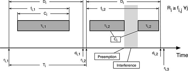
FIGURE 11.1
Notation for real-time scheduling algorithms and analysis methods.
As shown in the figure, it is important to distinguish among the worst-case execution time of task τi, denoted by Ci, the response time of its j-th instance fi,j, and its worst-case response time, denoted by Ri. The worst-case execution time is the time required to complete the task without any interference from other activities, that is, if the task being considered were alone in the system.
The response time may (and usually will) be longer due to the effect of other tasks. As shown in the figure, a higher-priority task becoming ready during the execution of τi will lead to a preemption for most scheduling algorithms, so the execution of τi will be postponed and its completion delayed. Moreover, the execution of any tasks does not necessarily start as soon as they are released, that is, as soon an they become ready for execution.
It is also important to clearly distinguish between relative and absolute deadlines. The relative deadline Di is defined for task τi as a whole and is the same for all instances. It indicates, for each instance, the distance between its release time and the deadline expiration. On the other hand, there is one distinct absolute deadline di,j for each task instance τi,j. Each of them denotes the instant in which the deadline expires for that particular instance.
11.2 The Cyclic Executive
The cyclic executive, also known as timeline scheduling or cyclic scheduling, is one of the most ancient, but still widely used, real-time scheduling methods or algorithms. A full description of this scheduling model can be found in Reference [11].
TABLE 11.2
A simple task set to be executed by a cyclic executive
| Task τi | Period Ti (ms) | Execution time Ci (ms) |
| τ1 | 20 | 9 |
| τ2 | 40 | 8 |
| τ3 | 40 | 8 |
| τ4 | 80 | 2 |
In its most basic form, it is assumed that the basic model just introduced holds, that is, there is a fixed set of periodic tasks. The basic idea is to lay out offline a completely static schedule such that its repeated execution causes all tasks to run at their correct rate and finish within their deadline. The existence of such a schedule is also a proof “by construction” that all tasks will actually and always meet their deadline at runtime. Moreover, the sequence of tasks in the schedule is always the same so that it can be easily understood and visualized.
For what concerns its implementation, the schedule can essentially be thought of as a table of procedure calls, where each call represents (part of) the code of a task. During execution, a very simple software component, the cyclic executive, loops through the table and invokes the procedures it contains in sequence. To keep the executive in sync with the real elapsed time, the table also contains synchronization points in which the cyclic executive aligns the execution with a time reference usually generated by a hardware component.
In principle, a static schedule can be entirely crafted by hand but, in practice, it is desirable for it to adhere to a certain well-understood and agreed-upon structure, and most cyclic executives are designed according to the following principles. The complete table is also known as the major cycle and is typically split into a number of slices called minor cycles, of equal and fixed duration.
Minor cycle boundaries are also synchronization points: during execution, the cyclic executive switches from one minor cycle to the next after waiting for a periodic clock interrupt. As a consequence, the activation of the tasks at the beginning of each minor cycle is synchronized with the real elapsed time, whereas all the tasks belonging to the same minor cycle are simply activated in sequence. The minor cycle interrupt is also useful in detecting a critical error known as minor cycle overrun, in which the total execution time of the tasks belonging to a certain minor cycle exceeds the length of the cycle itself.
As an example, the set of tasks listed in Table 11.2 can be scheduled on a single-processor system as shown in the time diagram of Figure 11.2. If deadlines are assumed to be the same as periods for all tasks, from the figure it can easily be seen that all tasks are executed periodically, with the right period, and they all meet their deadlines.
More in general, this kind of time diagram illustrates the job that each processor in the system is executing at any particular time. It is therefore useful to visualize and understand how a scheduling algorithm works in a certain scenario. For this reason, it is a useful tool not only for cyclic executives but for any scheduling algorithm.
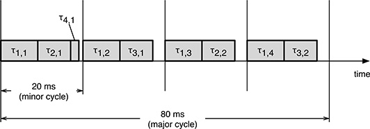
FIGURE 11.2
An example of how a cyclic executive can successfully schedule the task set of Table 11.2.
To present a sample implementation, we will start from a couple of quite realistic assumptions:
The underlying hardware has a programmable timer, and it can be used as an interrupt source. In particular, the abstract function
void timer_setup(int p)can be used to set the timer up, start it, and ask for a periodic interrupt with periodpmilliseconds.The function
void wait_for_interrupt(void)waits for the next timer interrupt and reports an error, for instance, by raising an exception, if the interrupt arrived before the function was invoked, denoting an overrun.The functions
void task_1(void), ...,void task_4()contain the code of tasks τ1, ..., τ4, respectively.
The cyclic executive can then be implemented with the following program.
int main( int argc, void * argv [])
{
  ...
  timer_setup(20);
  while (1)
  {
    wait_for_interrupt();
      task_1 ();
      task_2 ();
      task_4 ();
   wait_for_interrupt();
     task_1 ();
     task_3 ();
  wait_for_interrupt();
    task_1 ();
    task_2 ();
  wait_for_interrupt();
    task_1 ();
    task_3 ();
  }
}
In the sample program, the scheduling table is actually embedded into the main loop. The main program first sets up the timer with the right minor cycle period and then enters an endless loop. Within the loop, the function wait_for_interrupt() sets the boundary between one minor cycle and the next. In between, the functions corresponding to the task instances to be executed within the minor cycle are called in sequence.
Hence, for example, the first minor cycle contains a call to task_1(), task_2(), and task_4() because, as it can be seen on the left part of Figure 11.2, the first minor cycle must contain one instance of τ1, τ2, and τ4.
With this implementation, no actual processes exist at run-time because the minor cycles are just a sequence of procedure calls. These procedures share a common address space, and hence, they implicitly share their global data. Moreover, on a single processor system, task bodies are always invoked sequentially one after another. Thus, shared data do not need to be protected in any way against concurrent access because concurrent access is simply not possible.
Once a suitable cyclic executive has been constructed, its implementation is straightforward and very efficient because no scheduling activity takes place at run-time and overheads are very low, without precluding the use of a very sophisticated (and computationally expensive) algorithm to construct the schedule. This is because scheduler construction is done completely offline.
On the downside, the cyclic executive “processes” cannot be protected from each other, as regular processes are, during execution. It is also difficult to incorporate nonperiodic activities efficiently into the system without changing the task sequence.
11.3 Choice of Major and Minor Cycle Length
The minor cycle is the smallest timing reference of the cyclic executive because task execution is synchronized with the real elapsed time only at minor cycle boundaries. As a consequence, all task periods must be an integer multiple of the minor cycle period. Otherwise, it would be impossible to execute them at their proper rate.
On the other hand, it is also desirable to keep the minor cycle length as large as possible. This is useful not only to reduce synchronization overheads but also to make it easier to accommodate tasks with a large execution time, as discussed in Section 11.4. It is easy to show that one simple way to satisfy both constraints is to set the minor cycle length to be equal to the Greatest Common Divisor (GCD) of the periods of the tasks to be scheduled. A more flexible and sophisticated way of selecting the minor cycle length is discussed in Reference [11].
TABLE 11.3
A task set in which a since task, τ4, leads to a large major cycle because its period is large
| Task τi | Period Ti (ms) | Execution time Ci (ms) |
| τ1 | 20 | 9 |
| τ2 | 40 | 8 |
| τ3 | 40 | 8 |
| τ4 | 400 | 2 |
If we call Tm the minor cycle length, for the example presented in the previous section we must choose
The cyclic executive repeats the same schedule over and over at each major cycle. Therefore, the major cycle must be big enough to be an integer multiple of all task periods, but no larger than that to avoid making the scheduling table larger than necessary for no reason. A sensible choice is to let the major cycle length be the Least Common Multiple (LCM) of the task periods. Sometimes this is also called the hyperperiod of the task set. For example, if we call TM the major cycle length, we have
11.4 Tasks with Large Period or Execution Time
In the previous section, some general rules to choose the minor and major cycle length for a given task set were given. Although they are fine in theory, there may be some issues when trying to put them into practice. For instance, when the task periods are mutually prime, the major cycle length calculated according to (11.2) has its worst possible value, that is, the product of all periods. The cyclic executive scheduling table will be large as a consequence.
Although this issue clearly cannot be solved in general—except by adjusting task periods to make them more favorable—it turns out that, in many cases, the root cause of the problem is that only one or a few tasks have a period that is disproportionately large with respect to the others. For instance, in the task set shown in Table 11.3, the major cycle length is
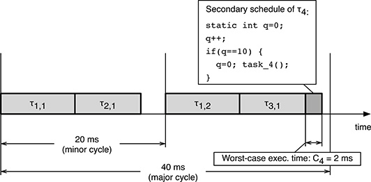
FIGURE 11.3
An example of how a simple secondary schedule can schedule the task set of Table 11.3 with a small major cycle.
However, if we neglected τ4 for a moment, the major cycle length would shrink by an order of magnitude
If τ4’s period T4 is a multiple of the new major cycle length , that is, if
the issue can be circumvented by designing the schedule as if τ4 were not part of the system, and then using a so-called secondary schedule.
In its simplest form, a secondary schedule is simply a wrapper placed around the body of a task, task_4() in our case. The secondary schedule is invoked on every major cycle and, with the help of a private counter q that is incremented by one at every invocation, it checks if it has been invoked for the k-th time, with k = 10 in our example. If this is not the case, it does nothing; otherwise, it resets the counter and invokes task_4(). The code of the secondary schedule and the corresponding time diagram are depicted in Figure 11.3.
As shown in the figure, even if the time required to execute the wrapper itself is negligible, as is often the case, the worst-case execution time that must be considered during the cyclic executive design to accommodate the secondary schedule is still equal to the worst-case execution time of τ4, that is, C4. This is an extremely conservative approach because task_4() is actually invoked only on every k iterations of the schedule, and hence, the worst-case execution time of the wrapper is very different from its mean execution time.
A different issue may occur when one or more tasks have a large execution time. The most obvious case happens when the execution time of a task is greater than the minor cycle length so that it simply cannot fit into the schedule. However, there may be subtler problems as well. For instance, for the task set shown in Table 11.4, the minor and major cycle length, chosen according to the rules given in Section 11.3, are
TABLE 11.4
Large execution times, of τ3 in this case, may lead to problems when designing a cyclic executive
| Task τi | Period Ti (ms) | Execution time Ci (ms) |
| τ1 | 25 | 10 |
| τ2 | 50 | 8 |
| τ3 | 100 | 20 |
In this case, as shown in the upper portion of Figure 11.4, task instance τ3,1 could be executed entirely within a single minor cycle because C3 ≤ Tm, but this choice would hamper the proper schedule of other tasks, especially τ1. In fact, the first instance of τ1 would not fit in the first minor cycle because C1 + C3 > Tm. Shifting τ3,1 into another minor cycle does not solve the problem either.
Hence, the only option is to split τ3,1 into two pieces: τ3,1a and τ3,1b, and put them into two distinct minor cycles. For example, as shown in the lower part of Figure 11.4, we could split τ3,1 into two equal pieces with an execution time of 10 ms each and put them into the first and third minor cycle, respectively.
Although it is possible to work out a correct cyclic executive in this way, it should be remarked that splitting tasks into pieces may cut across the tasks in a way that has nothing to do with the structure of the code itself. In fact, the split is not made on the basis of some characteristics of the code but merely on the constraints the execution time of each piece must satisfy to fit into the schedule.
Moreover, task splits make shared data management much more complicated. As shown in the example of Figure 11.4—but this is also true in general—whenever a task instance is split into pieces, other task instances are executed between those pieces. In our case, two instances of task τ1 and one instance of τ2 are executed between τ3,1a and τ3,1b. This fact has two important consequences:
If τ1 and/or τ2 share some data structures with τ3, the code of τ3,1a must be designed so that those data structures are left in a consistent state at the end of τ3,1a itself. This requirement may increase the complexity of the code.
It is no longer completely true that shared data does not need to be protected against concurrent access. In this example, it is “as if” τ3 were preempted by τ1 and τ2 during execution. If τ1 and/or τ2share some data structures with τ3, this is equivalent to a concurrent access to the shared data. The only difference is that the preemption point is always the same (at the boundary between τ3,1a and τ3,1b) and is known in advance.
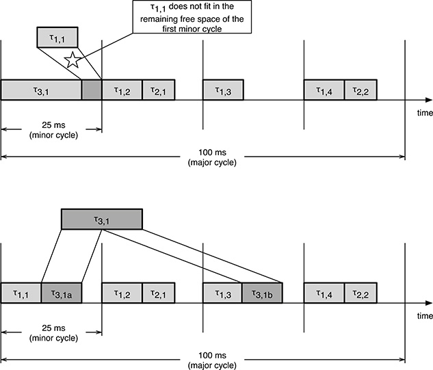
FIGURE 11.4
In some cases, such as for the task set of Table 11.4, it is necessary to split one or more tasks with a large execution time into pieces to fit them into a cyclic executive.
Last but not least, building a cyclic executive is mathematically hard in itself. Moreover, the schedule is sensitive to any change in the task characteristics, above all their periods, which requires the entire scheduling sequence to be reconstructed from scratch when those characteristics change.
Even if the cyclic executive approach is a simple and effective tool in many cases, it may not be general enough to solve all kinds of real-time scheduling problems that can be found in practice. This reasoning led to the introduction of other, more sophisticated scheduling models, to be discussed in the following chapters. The relative advantages and disadvantages of cyclic executives with respect to other scheduling models have been subject to considerable debate. For example, Reference [62] contains an in-depth comparison between cyclic executives versus fixed-priority, task-based schedulers.
11.5 Summary
To start discussing about real-time scheduling, it is first of all necessary to abstract away, at least at the beginning, from most of the complex and involved details of real concurrent systems and introduce a simple process model, more suitable for reasoning and analysis. In a similar way, an abstract scheduling model specifies a scheduling algorithm and its associated analysis methods without going into the fine details of its implementation.
In this chapter, one of the simplest process models, called the basic process model, has been introduced, along with the nomenclature associated with it. It is used throughout the book as a foundation to talk about the most widespread real-time scheduling algorithms and gain an insight into their properties. Since some of its underlying assumptions are quite unrealistic, it will also be progressively refined and extended to make it adhere better to what real-world processes look like.
Then we have gone on to specify how one of the simplest and most intuitive real-time scheduling methods, the cyclic executive, works. Its basic idea is to lay out a time diagram and place task instances into it so that all tasks are executed periodically at their proper time and they meet their timing constraints or deadlines.
The time diagram is completely built offline before the system is ever executed, and hence, it is possible to put into action sophisticated layout algorithms without incurring any significant overhead at runtime. The time diagram itself also provides intuitive and convincing evidence that the system really works as intended.
That said, the cyclic executive also has a number of disadvantages: it may be hard to build, especially for unfortunate combinations of task execution times and periods, it is quite inflexible, and may be difficult to properly maintain it when task characteristics are subject to change with time or the system complexity grows up. For this reason, we should go further ahead and examine other, more sophisticated, scheduling methods in the next chapters.