
16
Self-Suspension and Schedulability Analysis
CONTENTS
16.1 Self-Suspension and the Critical Instant Theorem
16.2 Self-Suspension and Task Interaction
The schedulability analysis techniques presented in Chapters 12 through 14 are based on the hypothesis that task instances never block for any reason, unless they have been executed completely and the next instance has not been released yet. In other words, they assume that a task may only be in three possible states:
ready for execution, but not executing because a higher-priority task is being executed on its place,
executing, or
not executing, because its previous instance has been completed and the next one has not been released yet.
Then, in Chapter 15, we analyzed the effects of task interaction on their worst-case response time and schedulability. In particular, we realized that when tasks interact, even in very simple ways, they must sometimes block themselves until some other tasks perform a certain action. The purpose of this extension was to make our model more realistic and able to better represent the behavior of real tasks. However, mutual exclusion on shared data access was still considered to be the only source of blocking in the system.
This is still not completely representative of what can happen in the real world where tasks also invoke external operations and wait for they completion. For instance, it is common for tasks to start an Input–Output (I/O) operation and wait until it completes or a timeout expires; another example would be to send a network message to a task residing on a different system and then wait for an answer.
More generally, all situations in which a task voluntarily suspends itself for a variable amount of time with a known upper bound—such as those just described—are called self-suspension or self-blocking. Therefore, in this chapter, the formulas to calculate the worst-case blocking time that may affect a task, given in Chapter 15, will be further extended to incorporate self-suspension. The extension is based on [76], addressing schedulability analysis in the context of real-time synchronization for multiprocessor systems.
16.1 Self-Suspension and the Critical Instant Theorem
At a first sight, it may seem that the effects of self-suspension should be local to the task that is experiencing it: after all, the task is neither competing for nor consuming any processor time while it is suspended, and hence, it should not hinder the schedulability of any other task because of this. This is unfortunately not true and, although this sounds counterintuitive, it turns out that adding a self-suspension region to a higher-priority task may render a lower-priority task no longer schedulable.
Even the critical instant theorem, on which many other theorems given in Chapter 12 are based, is no longer directly applicable to compute the worst-case interference that a task may be subject to. A counterexample is shown in Figure 16.1.
The upper part of the figure shows how two tasks τ1 (high priority) and τ2 (low priority) are scheduled when self-suspension is not allowed. Task τ1 has a period of T1 = 7 time units and an execution time of C1 = 4 time units. The uppermost time diagram shows how it is executed: as denoted by the downward-pointing arrows, its first three instances are released at t = 0, t = 7, and t = 14 time units, and since they have a priority higher than τ2, they always run to completion immediately after being released.
Time diagram A shows instead how the first instance of task τ2 is executed when it is released at t = 7 time units. This is a critical instant for τ2, because τ1,2 (the second instance of τ1) has been released at the same time, too. The execution time of C2 = 6 time units is allotted to τ2,1 in two chunks—from t = 11 to t = 14, and from t = 18 to t = 21 time units—because of the interference due to τ1.
Accordingly, the response time of τ2,1 is 14 time units. If the period of τ2 is T2 = 15 time units and it is assumed that its relative deadline is equal to the period, that is D2 = T2, then τ2,1 meets its deadline. The total amount of interference experienced by τ2,1 in this case is I2 = 8 time units, corresponding to two full executions of τ1 and shown in the figure as light grey rectangles. According to the critical instant theorem, this is the worst possible interference τ2 can ever experience, and we can also conclude that τ2 is schedulable.
As shown in time diagram B, if τ2,1 is not released at a critical instant, the interference will never be greater than 8 time units. In that time diagram, τ2,1 is released at t = 4 time units, and it only experiences 4 time units of interference due to τ1. Hence, as expected, its response time is 10 time units, less than the worst case value calculated before and well within the deadline.
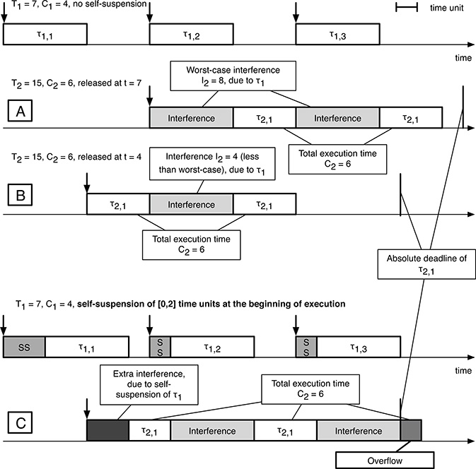
FIGURE 16.1
When a high-priority task self-suspends itself, the response time of lower-priority tasks may no longer be the worst at a critical instant.
The lower part of Figure 16.1 shows, instead, what happens if each instance of τ1 is allowed to self-suspend for a variable amount of time, between 0 and 2 time units, at the very beginning of its execution. In particular, the time diagrams have been drawn assuming that τ1,1 self-suspends for 2 time units, whereas τ1,2 and τ1,3 self-suspend for 1 time unit each. In the time diagram, the self-suspension regions are shown as grey rectangles. Task instance τ2,1 is still released as in time diagram B, that is, at t = 4 time units.
However, the scheduling of τ2,1 shown in time diagram C is very different than before. In particular,
The self-suspension of τ1,1, lasting 2 time units, has the local effect of shifting its execution to the right of the time diagram. However, the shift has a more widespread effect, too, because it induces an “extra” interference on τ2,1 that postpones the beginning of its execution. In Figure 16.1, this extra interference is shown as a dark gray rectangle.
Since its execution has been postponed, τ2,1 now experiences 8 time units of “regular” interference instead of 4 due to τ1,2 and τ1,3. It should be noted that this amount of interference is still within the worst-case interference computed using the critical instant theorem.
The eventual consequence of the extra interference is that τ2,1 is unable to conclude its execution on time and overflows its deadline by 1 time unit.
In summary, the comparison between time diagrams B and C in Figure 16.1 shows that the same task instance (τ2,1 in this case), released at the same time, is or is not schedulable depending on the absence or presence of self-suspension in another, higher-priority task (τ1).
On the other hand, the self-suspension of a task cannot induce any extra interference on higher-priority tasks. In fact, any lower-priority task is immediately preempted as soon as a higher-priority task becomes ready for execution, and cannot interfere with it in any way.
The worst-case extra interference endured by task τi due to its own self-suspension, as well as the self-suspension of other tasks, can be modeled as an additional source of blocking that will be denoted . As proved in [76], can be written as
where Si is the worst-case self-suspension time of task τi and, as usual, hp(i) denotes the set of task indexes with a priority higher than τi.
According to this formula, the total blocking time due to self-suspension endured by task τi is given by the sum of its own worst-case self-suspension time Si plus a contribution from each of the higher-priority tasks. The contribution of task τj to is given by its worst-case self-suspension time Sj, but it cannot exceed its execution time Cj.
In the example, from (16.1) we have
because the worst-case self-suspension time of τ1 is indeed 2 time units and the set hp(1) is empty.
Moreover, it is also
because τ2 never self-suspends itself (thus S2 = 0) but may be affected by the self-suspension of τ1 (in fact, hp(2) = {1}) for up to 2 time units.
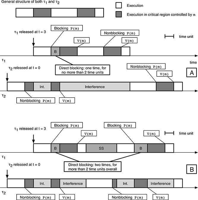
FIGURE 16.2
When a task self-suspends itself, it may suffer more blocking than predicted by the theorems of Chapter 15.
16.2 Self-Suspension and Task Interaction
The self-suspension of a task has an impact on how it interacts with other tasks, and on the properties of the interaction, too. That is, many theorems about the worst-case blocking time proved in Chapter 15, lose part of their validity when tasks are allowed to self-suspend.
Figure 16.2 shows how two periodic, interacting tasks, τ1 and τ2, are scheduled with and without allowing self-suspension. The general structure of a task instance is the same for both tasks and is shown in the uppermost part of the figure:
The total execution time of a task instance is C1 = C2 = 10 time units and comprises two critical regions.
At the beginning, the task instance executes for 2 time units.
Then, it enters its first critical region, shown as a dark grey rectangle in the figure. If we are using a semaphore
mfor synchronization, the critical region is delimited, as usual, by the primitivesP(m)(at the beginning) andV(m)(at the end).The task instance executes within the first critical region for 2 time units.
After concluding its first critical region, the task instance further executes for 3 time units before entering its second critical region.
It stays in the second critical region for 2 time units.
After the end of the second critical region, the task instance executes for 1 more time unit, and then it concludes.
Time diagram A of Figure 16.2 shows how the two tasks are scheduled, assuming that τ1 is released at t = 3 time units, τ2 is released at t = 0 time units, and the priority of τ1 is higher than the priority of τ2. It is also taken for granted that the period of both tasks is large enough—let us say T1 = T2 = 30 time units—so that only one instance of each is released for the whole length of the time diagram, and no self-suspension is allowed. In particular,
Task τ2 is executed from t = 0 until t = 3 time units. At t = 2, it enters its first critical region without blocking because no other task currently holds the mutual exclusion semaphore
m.At t = 3, τ2 is preempted because τ1 is released and hence becomes ready for execution. The execution of τ1 lasts 2 time units until it blocks at the first critical region’s boundary with a blocking
P(m).Task τ2 resumes execution (possibly with an increased active priority if either priority inheritance or priority ceiling are in use) until it exits from the critical region at t = 6 time units.
At this time, τ1 resumes—after 1 time unit of direct blocking—and is allowed to enter into its first critical region. From this point on, the current instance of τ1 runs to run completion without blocking again.
Thereafter, the system resumes τ2 and concludes it.
It should be noted that the system behavior, in this case, can still be accurately predicted by the theorems of Chapters 12 through 15, namely:
The interference underwent by τ2 (the lower-priority task) is equal to the worst-case interference predicted by the critical instant theorem and Response Time Analysis (RTA), that is, C1 = 10 time units. In Figure 16.2, interference regions are shown as light gray rectangles. Thus, the response time of τ2 is 20 time units, 10 time units of execution plus 10 time units of interference.
Task τ1 (the higher-priority task) does not suffer any interference due to τ2; it undergoes blocking, instead. We know that τ1 may block at most once, due to Lemmas 15.2, Lemma 15.5, or Theorem 15.1 (for priority inheritance), as well as Theorem 15.4 (for priority ceiling).
The worst-case blocking time can be calculated by means of Theorem 15.2 (for priority inheritance), or Theorem 15.5 (for priority ceiling). The result is the same in both cases and is equal to the maximum execution time of τ2 within a critical region, that is, 2 time units. In the example, τ1 only experiences 1 time unit of blocking, less than the worst case. Accordingly, the response time of τ1 is 11 time units, 10 time units of execution plus 1 time unit of direct blocking.
Time diagram B of Figure 16.2 shows instead what happens if task τ1 self-suspends for 3.5 time units after 5 time units of execution:
Task τ2 is now executed while τ1 is suspended, but it is still subject to the same total amount of interference as before. Therefore, unlike in the example discussed in Section 16.1, the response time of τ2 stays the same in this case.
The scheduling of τ1 is radically different and implies an increase of its response time, well beyond the additional 3.5 time units due to self-suspension. In fact, the response time goes from 11 to 16 time units.
The reason for this can readily be discerned from the time diagram. When τ1 is resumed after self-suspension and tries to enter its second critical region, it is blocked again because τ2 entered its second critical region while τ1 itself was suspended.
The second block of τ1 lasts for 1.5 time units, that is, until τ2 eventually exits from the second critical region and unblocks it.
The total response time of τ1 is now given by 10 time units of execution plus 3.5 time units of self-suspension (the gray block marked SS in the figure) plus 2.5 time units of blocking time (the two gray blocks marked B). In particular, 1 time unit of blocking is due to the first block and 1.5 units to the second one.
In summary,
It is no longer true that τ1 may block at most once. In fact, τ1 was blocked twice in the example. As a consequence, it is clear that Lemmas 15.2, Lemma 15.5, and Theorem 15.1 (for priority inheritance), as well as Theorem 15.4 (for priority ceiling) are no longer valid.
Similarly, Theorem 15.2 (for priority inheritance) and Theorem 15.5 (for priority ceiling) are no longer adequate to compute the worst-case blocking time of τ1. Even in this simple example, we have just seen that the total blocking time of τ1 is 2.5 time units, that is, more than the 2 time units of worst-case blocking time predicted by those theorems.
There are several different ways to take self-suspension into account during worst-case blocking time calculation. Perhaps the most intuitive one, presented in References [61, 76], considers task segments—that is, the portions of task execution delimited by a self-suspension—to be completely independent from each other for what concerns blocking. Stated in an informal way, it is as if each task went back to the worst possible blocking scenario after each self-suspension.
In the previous example, τ1 has two segments because it contains one self-suspension. Thus, each of its instances executes for a while (this is the first segment), self-suspends, and then executes until it completes (second segment). More generally, if task τi contains Qi self-suspensions, it has Qi +1 segments.
According to this approach, let us call B1S i the worst-case blocking time calculated as specified in Chapter 15, without taking self-suspension into account; that is,
or
where, as before,
K is the total number of semaphores in the system.
usage(k, i) is a function that returns 1 if semaphore Sk is used by (at least) one task with a priority less than τi and (at least) one task with a priority higher than or equal to τi; otherwise, it returns 0.
C(k) is the worst-case execution time among all critical regions guarded by semaphore Sk.
This quantity now becomes the worst-case blocking time endured by each individual task segment. Therefore, the total worst-case blocking time of task τi due to task interaction, , is given by
where Qi is the number of self-suspensions of task τi.
In our example, from either (16.4) or (16.5) we have
because the worst-case execution time of any task within a critical region controlled by semaphore m is 2 time units and τ1 can be blocked by τ2.
We also have
because τ2 is the lowest-priority task in the system and cannot be blocked by any other task. In fact, usage(k, 2) = 0 for any k.
According to (16.6), the worst-case blocking times are
for τ1, and
for τ2. This is of course not a formal proof, but it can be seen that is indeed a correct upper bound of the actual amount of blocking seen in the example.
An additional advantage of this approach is that it is very simple and requires very little knowledge about task self-suspension itself. It is enough to know how many self suspensions each task contains, information quite easy to collect. However, the disadvantage of using such a limited amount of information is that it makes the method extremely conservative. Thus, is not a tight upper bound for the worst-case blocking time and may widely overestimate it in some cases.
More sophisticated and precise methods do exist, such as that described in Reference [54]. However, as we have seen in several other cases, the price to be paid for a tighter upper bound for the worst-case blocking is that much more information is needed. For instance, in the case of [54], we need to know not only how many self suspensions each task has got, but also their exact location within the task. In other words, we need to know the execution time of each, individual task segment, instead of the task execution time as a whole.
16.3 Extension of the Response Time Analysis Method
In the basic formulation of RTA given in Chapter 14, the worst-case response time Ri of task τi was expressed according to (14.1) as
where Ci is its execution time, and Ii is the worst-case interference the task may experience due to the presence of higher-priority tasks.
Then, in Chapter 15, we argued that the same method can be extended to also handle task interactions—as well as the blocking that comes from them—by considering an additional contribution to the worst-case response time as written in (15.1):
where Bi is the worst-case blocking time of τi. It can be proved that (16.12) still holds even when tasks are allowed to self-suspend, if we redefine Bi to include the additional sources of blocking discussed in Sections 16.1 (extra interference) and 16.2 (additional blocking after each self-suspension).
Namely, Bi must now be expressed as:
In summary, referring to (16.1) and (16.6) for the definition of and , respectively, and then to (16.4) and (16.5) for the definition of , we can write
for priority inheritance, as well as
for priority ceiling.
The recurrence relationship used by RTA and its convergence criteria are still the same as (15.2) even with this extended definition of Bi, that is,
A suitable seed for the recurrence relationship is
Let us now apply the RTA method to the examples presented in Sections 16.1 and 16.2. Table 16.1 summarizes the attributes of the tasks shown in Figure 16.1 as calculated so far. The blocking time due to task interaction, , is obviously zero for both tasks in this case, because they do not interact in any way.
For what concerns the total blocking time Bi, from (16.13) we simply have:
TABLE 16.1
Attributes of the tasks shown in Figure 16.1 when τ1 is allowed to self-suspend
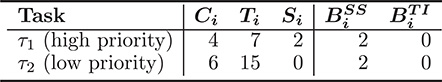
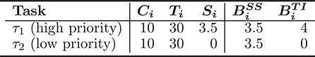
TABLE 16.2
Attributes of the tasks shown in Figure 16.2 when τ1 is allowed to self-suspend
For τ1, the high-priority task, we simply have
and the succession converges immediately. Therefore, it is R1 = 6 time units. On the other hand, for the low-priority task τ2, it is
Therefore, it is R2 = 20 time units.
Going to the second example, Table 16.2 summarizes the attributes of the tasks shown in Figure 16.2. The worst-case blocking times due to task interaction have already been derived in Section 16.2, while the worst-case blocking times due to self-suspension, , can be calculated using (16.1) as:
The total blocking time to be considered for RTA is therefore:
As before, the high-priority task τ1 does not endure any interference, and hence, we simply have:
and the succession converges immediately, giving R1 = 17.5 time units. For the low-priority task τ2, we have instead:
The worst-case response time of τ2 is therefore R2 = 23.5 time units.
16.4 Summary
This chapter complements the previous one and further extends the schedulability analysis methods at our disposal to also consider task self-suspension. This is a rather common event in a real-world system because it occurs whenever a task voluntarily suspends itself for a certain variable, but upper-bounded, amount of time. A typical example would be a task waiting for an I/O operation to complete.
Surprisingly, we saw that the self-suspension of a task has not only a local effect on the response time of that task—this is quite obvious—but it may also give rise to an extra interference affecting lower-priority tasks, and further increase the blocking times due to task interaction well beyond what is predicted by the analysis techniques discussed in Chapter 15.
The main goal of the chapter was therefore to look at all these effects, calculate their worst-case contribution to the blocking time of each task, and further extend the RTA method to take them into account. This last extension concludes our journey to make our process model, as well as the analysis techniques associated with it, closer and closer to how tasks really behave in an actual real-time application.