
4 Optimizing Discrete Modeling and Simulation for Real-Time Constraints with Metaprogramming
Luc Touraille, Jonathan Caux and David Hill
CONTENTS
4.2 Code Generation and Metaprogramming for Optimizing Real-Time Simulation
4.2.1 Concepts and Definitions
4.2.2.2 Instructions Generation
4.2.3 Domain-Specific Languages
4.2.4 Multistage Programming Languages
4.2.4.1 C++ Template Metaprogramming
4.2.6 Comparison of the Different Approaches
4.3 Application to Simulation: DEVS-Metasimulator
4.1 Introduction
Real-time simulation is characterized by the strong constraints that must be respected regarding the time spent simulating an activity. Usually we can run simulation faster than real time, and we synchronize with virtual time with techniques that are now mastered by many engineers [1]. Sometimes, the simulation can execute at a higher rate than the actual system evolves; in this case, all that is necessary is delaying the simulation so that virtual time stays synchronized to the expected wall clock real time. However, when the simulation involves heavy computation or the simulated activities are very short-lived, meeting the deadlines may imply optimizing certain parts of the simulation to reduce its execution time. A simulation run that is slower than real time can occur when dealing with detailed physical models. For instance, we experienced this when simulating the details of particles for physical studies in nuclear medicine [2,3]. In these works, we faced modeling cases where it was impossible to meet the real-time constraints. Medical scanning experiments that last 20–30 minutes can be simulated in a few seconds with analytical models. However, the results obtained can be very imprecise for small tumors (up to 100% error for tumors lesser than 1 cm in diameter). To be more precise, we must build 3D spatial stochastic models, which run for more than 9 hours on our current computer, and many replicates are necessary to reduce the error (less than 10% error achieved in 3 days of computing using the European Computing Grid) [4].
Even in simpler cases, achieving real-time simulation can be complicated. We have met such a case when dealing with fire spreading simulations following detailed physical experiments where physicists wanted to meet strong requirements in terms of both performance and precision. When a fixed spatial precision is set for the predictions obtained with fire spreading modeling, efficient models and high-performance computations are required [5]. The efficiency of discrete event simulators is now receiving significant attention [6, 7, 8 and 9].
In this chapter, we present a set of software engineering techniques for improving performance through code generation and metaprogramming for greater runtime efficiency. The gain obtained through such techniques enables reconsidering some simulation applications where it would be a distinct benefit to have precise human-in-the-loop simulations that are currently too slow to be considered for real-time applications. There are a number of optimization techniques that can be applied; in Section 4.2, we focus on what can be achieved with code generation and metaprogramming. After the introduction of several metaprogramming techniques, we propose a comparison to show the different benefits they provide regarding performance and design. Section 4.3 applies C++ Template Metaprogramming (TMP) to the Discrete Event System Specification (DEVS) in the simulation domain. We then close with some conclusions in Section 4.4.
4.2 Code Generation and Metaprogramming for Optimizing Real-Time Simulation
An intuitive and (most of the time) easily verifiable notion is that the more generic a program is, the less efficient it is. A solution that is especially tailored to answer a specific problem or small set of problems has a good chance of being more effective than a solution solving a bigger set of problems. For example, a piece of code computing the result of an equation will perform better than a full-fledged equation solver. However, this classic trade-off between abstraction/genericity and performance can be overcome to attain the best of both worlds by using metaprogramming and particularly dedicated program generation.
4.2.1 Concepts and Definitions
The simplest definition of a metaprogram is “a program that creates or manipulates a program.” This definition encompasses many concepts: source code generation, compilation, reflection, string evaluation, and so on. There is currently no broadly accepted taxonomy of metaprogramming systems. Two interesting propositions can be found in Refs. [10,11], where the authors identify concepts and relationships to characterize metaprograms. When dealing with performance, the most useful aspect of metaprogramming is program generation. Sheard [10] provides the following definition for a program generator:
A program generator (a meta-program) solves a particular problem by constructing another program (an object program) that solves the problem at hand. Usually, the generated (object) program is “specialized” for the particular problem and uses fewer resources than a general purpose, non-generator solution.
The definition by Damaševičius and Štuikys [11] is more general and simply states that
Software generation is an automated process of creation of a target system from a high-level specification.
These definitions are nicely encompassed by the concept of multistage programming [12], that is, decomposing the execution of a program into several steps. As Figure 4.1 shows through some examples, any kind of program execution can be seen as a sequence of steps. In particular, execution can be performed in a single stage (interpretation as in PHP program execution), two stages (e.g., compilation + execution), or more (e.g., code generation + compilation + execution).
Adding a new stage to the interpretation approach means reducing the abstraction level to finally produce a code optimized for performing the operations described in the source program. Optionally, each stage can be parameterized by an input other than the source specification. For example, a compiler produces a machine code corresponding to the input source code and specific and optimized for a specific target machine.
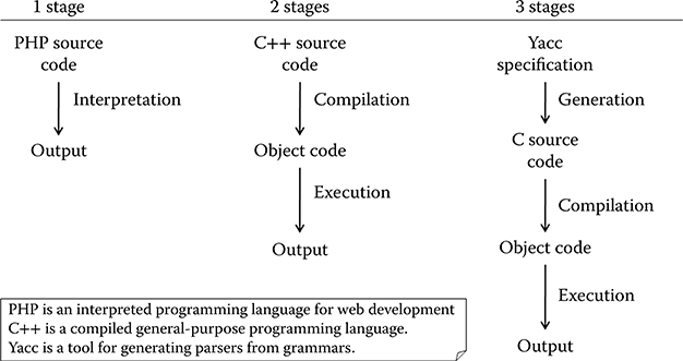
FIGURE 4.1 Samples of n-stage executions.
In Sections 4.2.2 to 4.2.5, we will present several metaprogramming techniques that allow the generation of specialized and optimized artifacts without sacrificing genericity and abstraction. We adopt a pragmatic point of view, so that emphasis will be on practical examples rather than on theoretical aspects.
4.2.2 Text Generation
Metaprogramming can be as simple as writing strings into a file. For example, the following C code is a metaprogram that generates a C file containing the code for printing the string passed to the metaprogram:
#include <stdio.h>
int main( int argc, char * argv[] )
{
FILE * output;
output = fopen( argv[1], “w” );
fprintf( output, “#include <stdio.h>
” ); fprintf( output, “int main(void)
” );
fprintf( output, “{
” );
fprintf( output, “ printf(“%s”);
”, argv[2] ); fprintf( output, “}” );
return 0;
}
CODE 1 C metaprogram generating C source code printing the string given in argument.
Of course, this contrived example adds little value compared to writing the object program directly. However, this technique becomes quite valuable when the object code is too tedious to write by hand or when the metaprogram performs computations on its arguments before generation as all the computations that are performed beforehand need not be executed in the object program. Compared to other metaprogramming techniques, a major advantage of source code generation is that the output is readable by a human, thereby helping debugging. However, the string approach presented here has the drawback that the validity of the object program cannot be enforced at the meta level.
We can make a distinction between two types of generation: data generation and instructions generation.
4.2.2.1 Data Generation
The aim of data generation is to compute a set of values before execution so that they are already loaded in memory when the program starts. For example, some programs use a lookup table containing the sine of many values instead of computing the sine each time it is needed. Most of the time, this lookup table is populated at start-up; however, a more efficient approach is to generate the code for initializing the lookup table directly with the correct values. This technique can also be used to accelerate stochastic simulation by having a metaprogram generate the pseudorandom numbers instead of generating the stream during execution. The metaprogram creates a file containing the initialization of an array with the generated numbers. This file can then be compiled and each simulation that must use the random stream only has to link to the object file obtained. In these programs, the time that it takes to obtain a pseudorandom number is significantly decreased (in previous work [13], we observed a factor of 5). This approach fits with the large memories we have even on personal computers since it favors execution time at the expense of additional object file space. When the amount of pseudorandom numbers is too large to be stored in memory, memory mapping techniques can be used [14,15].
4.2.2.2 Instructions Generation
With data generation, we mostly generate values. It is nevertheless metaprogramming, because we also generate the code to store these values in a data structure accessible at runtime. However, this is not the nominal use of metaprogramming. A metaprogram occasionally generates data, but mainly generates instructions. We can consider the metaprogram as a metasolution to a given problem. Instead of solving the problem, the program generates a solution to the problem. A metaprogram is often more generic than a regular program, and it can create solutions specialized for the inputs it receives. For example, in the work by Missaoui, Hill, and Perret [16], a metaprogram was used to generate programs for computing every reverse translation of oligopeptides containing a given set of amino acids. The metaprogram identified the set of amino acids to be considered as the input and generated a nonrecursive pile handling program with a big number of nested loops, used to compute the backtranslations of any oligopeptide (composed of the amino acids specified at generation). The resulting programs would have been difficult, if not impossible, to write manually without sacrificing some efficiency.
Both generation approaches have been used in the real-time context for decades. In the work by Auer, Kemppainen, Okkonen, and Seppänen [17], a code generator is presented to implement full tasks for real-time systems. The code is produced from a structured data/control flow description following the real-time structured analysis/ structured design (RT-SA/SD) methodology [18] and the program transformation paradigm (which is now a classical concept of the model-driven paradigm). Petri net programs and PL/M-x86 code were generated, and the resulting Petri nets were used for dynamic analysis, helping the discovery of significant errors hidden in the RT-SA/SD specifications. In the work by Webster, Levy, Harley, Woodward, Naidoo, Westhuizen, and Meyer [19], we find the generation of parallel real-time control code. A prototype of a controller hardware platform with the design and implementation of the associated software showed efficient real-time response with customized code generation for a set of particular processors. Parallelism was used to optimize real-time responses and to increase controller throughput.
4.2.3 Domain-Specific Languages
Domain-specific languages (DSLs) are programming or modeling languages dedicated to a particular domain. They contrast with general-purpose programming languages (GPLs) such as C, Java, and LISP and general-purpose modeling languages such as UML, which can be used in any domain. A DSL usually defines a textual or graphical syntax for manipulating the domain entities. Specifications written in the DSL are compiled either directly to machine code or more often to source code in a GPL.
The advantages of using DSLs are numerous. The most obvious is that they provide abstractions that are at the appropriate level for the user, hence expediting development of models and applications. However, the same effect can be more or less achieved in a GPL through libraries. More interesting are the opportunities that DSLs bring regarding verification and optimization. Indeed, since the language is domain-dependent, the tools for manipulating specifications can themselves be domain-dependent. This means that verification about the program can be performed at design time using domain knowledge. Similarly, the DSL compiler can perform several domain-specific optimizations [20]. For the sake of illustration, let us consider electronic circuit simulation. Using a traditional library,* the user would manipulate classes and functions. For example, there could be classes for representing each type of logical gate. When compiling this program, all the GPL compiler sees is classes and functions, and therefore, it is only able to perform generic optimizations such as loop unrolling and inlining. Now, if the same program were written in a DSL for circuit simulation (such as VHSIC Hardware Description Language (VHDL) [21]), the DSL compiler could perform more specific optimizations. For example, the DSL compiler could be aware that the combination of two NOT gates is equivalent to no gates at all and consequently avoid generating the code for these two gates in the object program.
DSLs have been used in simulation for a long time. In a previous work [22,23], we surveyed some of the most prominent simulation DSLs, which are briefly discussed in the current chapter. Back in the 1960s, IBM introduced GPSS (Global Purpose Simulation System [24]), a language for discrete event simulation with both a textual syntax and a graphical syntax, which could be compiled to machine code or to interpretable pseudocode. In the late 1970s, SLAM (Simulation Language for Alternative Modeling) [25] was introduced. It made it possible to use several modeling approaches (process, event, and continuous [26]), possibly combined together. A few years later, SIMAN (SIMulation ANalysis [27]) was released. It allowed modeling discrete, continuous, or hybrid systems and was used in several modeling and simulation software such as ARENA, which is still evolving and widely used. We can also cite the QNAP2 (Queuing Network Analysis Package 2 [28]) language, based on the theory of queuing networks. The trend in the past few years has been to make languages even more specialized. Indeed, the notion of specificity is rather subjective. After all, even though the above-mentioned languages seem more specific than a GPL such as FORTRAN or C, they can also be seen as much more generic than a DSL for flight simulation, for instance. The more specific a DSL is, the easier it is to use it and to perform verification and optimization on the model. However, it also greatly limits its scope. As a consequence, the cost of developing the DSL should not be higher than the outcome obtained by using it. Fortunately, there are more and more tools available to ease their development. One of the most active areas in this regard is model-driven engineering (MDE) [29,30]. Indeed, the MDE approach and the tools developed to support it enable, among other things, the creation of new DSLs in a very short time. DSLs are supported by providing metamodels and model transformations to develop abstract syntaxes, concrete syntaxes, code generators, graphical editors, and so on.
* “Traditional library” as opposed to “active library,” a notion that is presented later in this section.
Several DSLs have been developed for real-time programming; some of them target a broad range of real-time systems (e.g., Hume [31], or the graphical modeling language used in Simulink® [32]), while others are more specialized and are peculiar to a given business such as avionics [33] or robotics [34]. All these DSLs make it easier to write real-time applications by providing high-level constructs, for example, for describing time constraints in an operation. Moreover, these languages most of the time exhibit characteristics that are difficult to obtain with GPL, such as determinacy or bounded time/space. They can also outperform GPLs by applying domain-specific optimizations. For example, Simulink can minimize a certain type of loops in models, thereby removing the need to solve them at runtime with a computationally expensive loop solver.
4.2.3.1 Embedded DSLs
The development of a DSL from scratch can be quite cumbersome. Tools are available to facilitate the process, such as Lex and Yacc [35] or MDE-related tools, but it is still not a seamless experience. Moreover, the DSL puts some burden on the user who must learn an entirely new syntax and use some specific tools to generate or execute its code. Finally, it sometimes happens that a DSL must contain a GPL as a sublanguage to provide the user with complete flexibility on some part of a program (these are sometimes called hybrid DSLs).
An interesting approach to overcome these issues is the concept of embedded domain-specific languages (EDSLs), sometimes called internal DSLs [36]. These DSLs are embedded in a host language (usually a GPL), meaning that they are defined using the host constructs and syntax. This implies that every expression in the DSL must be a valid expression in the GPL. Even though this seems to be an unacceptable restriction, the gains obtained by using an EDSL are quite attractive:
The syntax is the same as the host GPL, and therefore, the user can focus on learning the DSL semantics.
The GPL can be used in synergy with the DSL to have both the practical expressivity of the DSL and the theoretical expressivity of the GPL.
It is not necessary to write a custom lexer, parser, and code generator because all of these are provided for the GPL and can be exploited at no additional charge for the DSL, including the generic optimizations performed by the GPL optimizer.
Fowler identified several techniques for writing DSLs in object-oriented languages and more broadly in any procedural language [36]. These techniques aim at providing a fluent interface to a library, meaning an API designed to flow like natural language: the code using the library should be readable as if it were written in a language of its own. Method chaining is one of the techniques that can be used to provide a fluent interface. Code 2 hereafter shows a sample of code for operating a robot that uses a fluent interface. The interface of the “Robot” class is designed so that the code using it can be read as if using a language specific to robot manipulation.
Robot wall_e;
wall_e.
right( 60 ).
forward().
length( 100 ).
speed( 20 ).
left( 20 ).
deployArm();
CODE 2 Sample use of a fluent interface for robot manipulation.
The syntax of the DSL can be even richer in languages that support operator overloading such as C++ and C# and/or operator definition such as Scala and F#. In the first case, the DSL designer can reuse existing operators in his/her own language to provide a more usable syntax, while in the second case, the designer can even create his/her own keywords to extend the original GPL syntax.
However, as enjoyable as providing a language-like interface to a library can be, it is not acceptable in the case at hand if it unfavorably affects performance. In general, providing a fluent interface implies additional runtime computations, notably to keep track of the context. Does it mean that EDSLs should not be employed when execution time is a concern? No, not if we couple the notion of EDSL with the one of active library. Veldhuizen and Gannon [37], who coined the term in 1998, provide the following definition:
Unlike traditional libraries which are passive collections of functions and objects, Active Libraries may generate components, specialize algorithms, optimize code [and] configure and tune themselves for a target machine […].
In other words, an active library can provide the same generic abstractions as a traditional one while at the same time providing maximum efficiency, thanks to code generation and optimization, achievable through metaprogramming. We can see an active library as a library generator that creates libraries tailored for the user-specific needs, depending on its parameterization.
Therefore, an EDSL implemented as an active library will be able to perform the same operations the compiler executes when dealing with external DSL. Ahead of execution, the library can perform abstract syntax tree rewriting, evaluation of constant expressions, domain-specific optimizations, and so on, effectively resulting in a code specialized for the user’s program. The languages providing the most powerful facilities for implementing “active EDSLs” are functional languages such as dialects of the LISP family, which provide macros for extending the syntax and quasiquoting/unquoting* for generating code, and languages with very flexible syntax such as Ruby or Scala. However, these languages are not as widely used as other languages such as Java or C, and their strength lies in aspects other than performance. On the contrary, the C++ language is one of the most used languages and exhibits some of the best performance. And the good news for this now “old” language is that it supports active libraries, EDSLs, and metaprogramming, through the use of the template mechanism, as will be discussed in Section 4.2.4.
* These terms will be defined in Section 4.2.4.
A pioneer in the area of C++ active EDSLs is Blitz++ [38], a scientific computing library that uses metaprogramming to optimize numerical computations at compile time, making it possible to equal and sometimes exceed the speed of FORTRAN. Since then, frameworks have been developed to facilitate the writing of C++ EDSL. The most accomplished one is probably Boost.Proto [39], a C++ EDSL for defining C++ EDSLs. This active library makes it extremely easy to define grammars, evaluate or transform expression trees, and so on, all in C++ and with most of the computation happening at compile time. It has been successfully exploited in several domains such as parsing and output generation (Boost.Spirit), functional programming (Boost.Phoenix), or parallel programming (Skell BE [40]).
In the real-time domain, most EDSLs are based on functional languages, which are more amenable to static analysis than imperative languages and easier to adapt into DSLs. A good example is Atom, a Haskell-based EDSL [41] that provides several guarantees such as deterministic execution time and memory consumption, notably by performing task scheduling and thread synchronization at compile time. A short overview of the available DSLs for real-time systems modeling can be found in Ref. [42].
4.2.4 Multistage Programming Languages
Multistage programming languages (MSPLs) are languages including constructs for concisely building object programs that are guaranteed to be syntactically correct [12].
In traditional programming languages, program generation is performed through either strings or data types manipulation. The first approach, presented at the beginning of this section, has the major drawback that there is no way of proving that the resulting program will be correct. After all, “obj.meth(arg)” and “î#%2$µ” are both strings, but the first one may have a meaning in the object program while the second will probably be an erroneous piece of code. This issue can be solved by using data types to represent the object program (e.g., manipulating instances of classes such as Class, Method, Expression, and Variable), but doing so makes the metaprogram much less readable and concise.
To overcome these problems, MSPLs contain annotations to indicate which pieces of code belong to the object program. These pieces of code will not be evaluated during execution and will simply be “forwarded” to the object program. They must nevertheless be valid code, hence providing syntactic verification of the object program at the meta level. This is the core of the LISP macros system, where the quote operator is used to annotate object code. More interestingly, dialects of the LISP family usually include a backquote (quasiquote in Scheme) operator. A backquoted expression, as a quoted expression, will be included in the object program, but it can also contain unquoted expressions that will be evaluated before being included.* Backquoted expressions can be nested to provide an arbitrary number of stages. The LISP code below provides an example of a power function that generates the code for computing xn for a fixed n. The pow function takes two parameters, the base x and the exponent n, and is recursively defined (x0 = 1, xn = x * xn−1). However, since the multiplication is backquoted, it will not be performed immediately. Instead, it will be included in the generated code. The two operands being unquoted (through the comma operator), they will be replaced by the result of their evaluation. Eventually, the pow function will generate unrolled code without recursive calls nor test for base case.
* A similar feature, command substitution, can be found in Unix shells. Incidentally, the character used to denote commands that must be substituted is also the backquote.
(define (pow x n)
(if (= n 0)
1
`(* ,x ,(pow x (- n 1)))
) )
(pow 'var 4)
;Output: (* var (* var (* var (* var 1))))
CODE 3 LISP Code generating the code computing xn.
This backquote feature, even though powerful, can create some issues regarding symbol binding. In particular, instead of being bound at the metaprogram level, they are bound during evaluation (in the object program), which is often not the desired behavior. The MetaML language [43] has been developed, among other reasons, to solve these problems.
Functional languages are well suited for metaprogramming, thanks to their homoiconicity (“data is code”), and have been successfully used to develop real-time applications. For instance, in the late 1980s, the expert system G2 was developed in Common LISP and heavily relied on macros to generate efficient code [44]. Thanks to that, this expert system was used for many soft real-time applications, including space shuttle monitoring and ecosystem control (Biosphere II).
However, functional languages are far from being mainstream and are not very well suited to computation-intensive simulations. More classic choices in this domain are C, C++, and Java. In these languages, an arbitrary number of stages would be difficult to achieve, although one of them still has some multistaging capability.
4.2.4.1 C++ Template Metaprogramming
C++, the well-known multiparadigm language, includes a feature for performing generic programming: templates. As a reminder, a class (resp. function) template is a parameterized model from which classes (resp. functions) will be generated during compilation, more precisely during a phase called template instantiation. This feature is very useful for writing generic classes (resp. functions) that can operate on any type or a set of types meeting some criteria. Moreover, templates proved to be more powerful than what was originally thought when they were introduced in the language. In 1994, Unruh found out that they could be used to perform numerical computations such as computing prime numbers, and Veldhuizen later established that templates were Turing complete [45]. These discoveries gave birth to a metaprogramming technique called C++ TMP [46].
Veldhuizen described C++ TMP as a kind of partial evaluation (see Section 4.2.5); however, it does not really correspond to the accepted definition. A more appropriate way to look at it would be to consider C++ with templates as a two and a half stage programming language: one stage and a half for template instantiation and compilation (which are in this case two indivisible steps), and one stage for execution.
C++ TMP exhibits several characteristics very close to functional programming, namely, lack of mutable variables, extensive use of recursion, and pattern matching through (partial) specialization. As an example, Code 4 hereafter presents the equivalent in C++ TMP of the LISP code shown above. The class template pow is parameterized by an exponent N. It contains a member function apply that takes as parameter a base x and multiplies it by xN−1. To do so, the template is instantiated with the decremented exponent, and the apply member function of this instantiation is invoked. The base case is handled through template specialization for N = 0. When the compiler encounters pow<4>::apply, it successively instantiates pow<3>::apply, pow<2>::apply, pow<1>::apply, and finally pow<0>::apply, which matches the specialization, hence stopping the recursion. Since the functions are small and simple, the compiler can inline them and remove the function calls, effectively resulting in a generated code that only performs successive multiplications.
template <unsigned int N>
struct pow
{
static double apply(double x)
{
return x * pow<N-1>::apply(x);
} };
template <>
struct pow<0>
{
static double apply(double x)
{
return 1;
}
};
[...]
double res = pow<4>::apply(var);
// the generated assembly code will be equivalent to
// var * var * var * var;
CODE 4 C++ template metaprogram for computing xn.
Writing metaprograms with C++ TMP is not as seamless an experience as it is in LISP or MetaML. The syntax is somewhat awkward since this usage of templates was not anticipated by the C++ Standards Committee. Fortunately, several libraries have been developed to smooth the process. The most significant ones are the MetaProgramming Library (MPL) and Fusion, two libraries belonging to the Boost repository. Boost.MPL is the compile-time equivalent of the C++ Standard Library. It provides several sequences, algorithms, and metafunctions for manipulating types during compilation. Boost.Fusion makes the link between compile-time metaprogramming and runtime programming, by providing a set of heterogeneous containers (tuples) that can hold elements with arbitrary types and several functions and algorithms operating on these containers either at compile time (type manipulation) or at runtime (value manipulation).
An application of C++ TMP to modeling and simulation is provided in Section 4.3.
4.2.5 Partial Evaluation
The last metaprogramming technique presented in this section is known as partial evaluation [47]. Partial evaluation is an automated form of multistage programming technique where the programmer is not required to invest any additional effort to obtain the benefit of program specialization.
In mathematics and computer science, partial application is the technique of transforming a function with several parameters to another function with a smaller arity where some of the parameters have been fixed to a given value. Partial evaluation is quite similar, except that it applies to programs instead of mathematical functions. A partial evaluator is an algorithm that takes as input a source program and some of its inputs, and generates a residual or specialized program. When run with the rest of the inputs, the residual program generates the same output as the original program. However, in the meantime, the partial evaluator had the opportunity to evaluate every part of the original program that depended on the provided inputs. Consequently, the residual program performs fewer operations than the source program, hence exhibiting better performance. Formally, we consider a program as a function of static and dynamic data given as input, which produces some output:
Given this definition, a partial evaluator can be defined as follows:
such that
As an example, in Code 5, C code of the binary search algorithm is shown. The algorithm recursively searches a given value in an ordered array and returns the index of the value (or −1 if it is not found).
int search( int * array, int value, int size )
{
return binary_search( array, value, 0, size-1 );
}
int binary_search( int * array, int value, int firstIndex, int lastIndex ) {
if ( lastIndex < firstIndex ) return −1; // value not found
int middleIndex = firstIndex + ( lastIndex – firstIndex ) / 2;
if ( array[ middleIndex ] == value ) // value found { return middleIndex;
}
else if ( array[ middleIndex ] > value ) // value is before {
return binary_search( array, value, firstIndex, middleIndex – 1 ); }
else // value is after
{ return binary_search( array, value, middleIndex + 1, lastIndex ); }
}
CODE 5 Binary search in C.
The search function takes three parameters: the ordered array, the searched value, and the size of the array. Assuming we have a means to partially evaluate this function, Code 6 shows the residual function we would obtain with size = 3.
int search3( int * array, int value ) {
if ( array[ 1 ] == value )
{
return 1;
}
else if ( array[ 1 ] > value ) {
if ( array[ 0 ] == value )
return 0; else
return −1;
}
else
{
if ( array[ 2 ] == value )
return 2; else
return −1;
} }
CODE 6 Binary search residual function for a given size (3).
In this residual function, partial evaluation eliminated all recursive calls, the computation of the middle index, and the test for the “value not found” base case. Most of the time, specializing a function or a program will yield a code that is both smaller and faster since many instructions will be eliminated. However, since partial evaluation performs operations such as loop unrolling and function inlining, it can sometimes lead to code bloat. This phenomenon, called overspecialization, should be avoided in the context of embedded programming. In addition to improving performance, the specialization of functions or programs can also be used to verify assertions about inputs before execution. The assertions will be checked by the partial evaluator, which will abort the residual program production if one of them is not verified.
At this point, it should be obvious that partial evaluation shares the same goal as other multistage programming techniques, namely, to produce an optimized version of a program, specialized for some data. The main difference is that the process of specialization is assigned to a partial evaluator, that is, a program that will automatically perform the generation. The partial evaluator is in charge of determining which pieces of data are static and hence can be exploited to perform ahead-of-time computations and which ones are dynamic (not known before runtime).
A partial evaluator operates in two main phases. First of all, it must annotate the input program to discriminate between eliminable and residual instructions. This step, called binding-time analysis, must ensure that the annotated program will be correct with respect to two requirements: congruence (every element marked as eliminable must be eliminable for any possible static input) and termination (for any static input, the specializer processing the annotated program must terminate). The second step actually performs the specialization by using several techniques, the most prominent ones being symbolic computation, function calls unfolding (inlining), and program point specialization (duplication of program parts with different specializations).
There are not many partial evaluators available yet. Most of the existing ones target declarative programming (notably functional and logic programming), where programs can be easily manipulated. However, there also exist partial evaluators for some imperative programming languages such as Pascal and C. Regarding more recent languages, it is interesting to mention a work that aims at providing a partial evaluator for the Common Intermediate Language [48]. This Common Intermediate Language is the pseudocode of the Microsoft .NET framework to which many high-level programming languages are compiled (C#, VB.NET, F#…).
Partial evaluation can sometimes be combined with other metaprogramming techniques. In the work by Herrmann and Langhammer [49], the authors apply both multistage programming (see Section 4.2.4) and partial evaluation to the interpretation of an image-processing DSL. Their interpreter first simplifies the original source code by partially evaluating it with some static input (the size of the image), then generates either bytecode or native code using staging annotations, before eventually executing the resulting program with the dynamic input (the image to be processed). Even though all these steps are performed at runtime, the improvement in execution time as compared with classical interpretation is extremely good, up to 100×.
In yet other work [50], partial evaluation is applied to real-time programs written for the Maruti real-time operating system to obtain deterministic execution times. Indeed, to be reusable, programs often must use features such as recursion or loop with nonbounded bounds that hinder the analysis of the program, notably the estimation of the execution time. The authors show that by partially evaluating these programs for some input, it is possible to remove the stochasticity inherent in these features and thereby obtain deterministic and predictable execution times.
4.2.6 Comparison of the Different Approaches
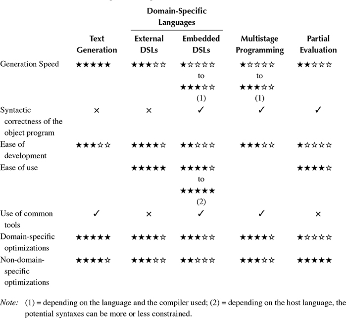
Table 4.1 presents a comparison of the metaprogramming techniques described previously. The criteria retained are as follows:
Generation speed: How fast the metaprogram generates the object program.
Syntactic correctness of the object program: Whether the syntactic validity of the object program is enforced at the metaprogram level (✓) or not (×).
Ease of development/Ease of use: How easy it is to create and use metaprograms. It is important to draw the distinction between these two activities, especially in the case of DSLs and partial evaluation. Indeed, most of the time, the people developing the tools and the ones using it will not be the same, and the work they have to provide will be very different. For instance, developing a partial evaluator is a distinctly difficult task, while developing an application and partially evaluating it is almost the same as writing a “classical” application, since partial evaluation is mostly automatic. Regarding text generation and multistage programming, we considered the case of ad-hoc programs developed with a particular aim in mind, not libraries. Consequently, it is irrelevant to differentiate between development and use.
Use of common tools: Whether the user can use widely available tools such as a compiler or an interpreter for a common language (C/C++, LISP…) (✓) or whether tools particular to the approach must be considered (×).
Domain-specific optimizations: Potential of the metaprogram for performing optimizations specific to the domain at hand (e.g., scheduling tasks ahead of runtime).
Non-domain-specific optimizations: Potential of the metaprogram for performing generic optimizations (e.g., unrolling a loop with a constant number of iterations). Only the optimizations performed by the metaprogram are considered, not the optimizations applied on the object program at a later stage (such as optimization during the compilation of generated source code).
Scores range from ★ to ★★★★★. Each criterion has been expressed so that a high score denotes an asset.
As can be seen from Table 4.1, there is no one-size-fits-all solution. Instead, each approach has its strengths and weaknesses, and selecting one must be done on a case-by-case basis, depending on the necessary features.
TABLE 4.1
Comparison of Metaprogramming Approaches
4.3 Application to Simulation: Devs-Metasimulator
In Section 4.2, we introduced several metaprogramming techniques for improving program performance. Hereafter, we present an application of one of these techniques, namely C++ TMP, to the simulation domain, more particularly to the Discrete EVent System specification (DEVS) formalism [51,6].
4.3.1 DEVS/RT-DEVS
The DEVS formalism was proposed by Zeigler in 1976. It establishes sound mathematical bases for modeling and simulation through three concepts: atomic models, coupled models, and abstract simulators. A DEVS atomic model is an entity holding a state and evolving through internal state changes and responses to external stimuli. After undergoing an internal event, the model generates an event that is sent to the “outside world.” Formally, a classic DEVS atomic model is defined by a 7-tuple:
where
X is the set of inputs. Usually, X is decomposed into several sets representing model ports.
Y is the set of outputs. It is defined similarly to X, using ports.
S is the state set, containing all the possible characterizations of the system.
ta is the time advance function. It determines how long the system stays in a given state before undergoing an internal transition and moving to another state.
δint is the internal state transition function. It defines how the system evolves in an autonomous way.
δext is the external state transition function. It defines how the system reacts when stimulated by an external event.
λ is the output function. Invoked after each internal transition, it determines the events generated by the system, functions of the state it was in.
Atomic models can be combined to form coupled models. A DEVS coupled model is a hierarchical structure composed of atomic and/or other coupled models. The components are organized in a graph-like structure where output ports of components are linked to input ports of other components. As such, output events generated by some components become input events to others. Formally, a classic DEVS coupled model is characterized by a structure
where
X is the set of input ports and values, as in atomic models.
Y is the set of output ports and values, as in atomic models. D is the set of component names.
For each d in D, Md is a DEVS model (coupled or atomic).
EIC is the external input coupling; it connects inputs of the coupled model N to component inputs.
EOC is the external output coupling; it connects component outputs to N outputs.
IC is the internal coupling; it connects component outputs to component inputs.
Select is the tie-breaking function. Classic DEVS is fundamentally sequential. Therefore, when two models are supposed to undergo an internal transition at the same time—and consequently generate two simultaneous events—only one of them must be activated. This arbitrage is performed through the Select function.
The operational semantic of these models have been defined through abstract simulators, which represent algorithms that correctly simulate DEVS models [51].
Many extensions have been proposed to increase the scope of DEVS: fuzzy-DEVS, dynamic structure DEVS, and so on. The real-time DEVS (RT-DEVS) [52] extension is particularly interesting in the context of this book. This formalism adapts classic DEVS to add real-time aspects and provides a framework for modeling systems and simulating them in real time so that they can interact with the physical world. As opposed to classic DEVS, an RT-DEVS simulator uses a real-time clock instead of a virtual one and hence must be deployed on a real-time operating system. The main idea is to fill the time between internal events with actual activities instead of virtually jumping through time.
The definition of RT-DEVS models is only slightly different than Classic DEVS models. Coupled models are specified in the same way, except for the lack of a Select function (which makes no sense in a real-time context, since in the physical world, events can occur simultaneously and are not “sequentialized”). Atomic models only differ in the addition of activities and the use of intervals to specify the time advance. An atomic RT-DEVS model is defined as follows:
where
X, Y, S, δint, δext, and λ are the same as in Classic DEVS.
A is a set of activities. An activity is a function, associated with a state, which must be fully executed before the state of the model can change.
ψ is the activity mapping function, which associates each state with an activity.
ti is the interval time advance function. It specifies, for each state, the estimated interval of time in which the associated activity is expected to be completed.
As for Classic DEVS, abstract simulators have been defined to characterize what must be done to execute RT-DEVS models. These simulators deal with concurrent execution of activities, simultaneous events, and so on. However, some timing discrepancies can appear during simulation. Indeed, simulators must execute not only the activities specified by the model but also the simulation operations necessary to make the model evolve during execution. This implies that, in addition to activities, the simulator must execute internal and external transition functions, output functions, event routing, and so on. Because of this overhead, timing errors can arise. More specifically, activities can start and finish later than they should. Algorithmic approaches have been proposed to compensate for these discrepancies [52]. However, these solutions only work when the duration of activities is larger than the simulation overhead. When activities are short, RT-DEVS models can run too slow to meet the constraints defined by the interval time advance function. Consequently, it is important to reduce the overhead as much as possible. Hereafter, we will explain how metaprogramming can improve the efficiency of DEVS simulators as well as other characteristics such as correctness.
4.3.2 Application of Metaprogramming to DEVS Simulation
DEVS models can be decomposed into structural specifications (ports, model composition, and couplings) and behavioral specifications (transition functions and output function). Most of the time, the structure will not change during execution (one notable exception are dynamic structure DEVS models). Consequently, the simulation of DEVS models appears to be a good candidate for metaprogramming optimizations. Previous work [53] presents a DEVS simulator, implemented as an active library, which specializes itself for the model provided using C++ TMP. The formalism handled by the simulator presented is Classic DEVS and the same ideas can be applied to DEVS extensions—such as RT-DEVS—or to other formalisms.
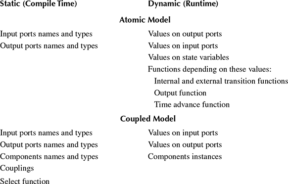
Table 4.2 classifies elements of DEVS models with respect to the earliest stage at which they are accessible. For example, the names of components in coupled models are static pieces of information (known at compile time) and can therefore be exploited in the metaprogram.
The “metasimulator” uses the static information to evaluate some parts of the simulation during template instantiation and generates a residual simulator specialized for the given model, where only the dynamic operations remain. Thanks to this, several improvements are obtained over more classical approaches that do not use metaprogramming.
A first set of enhancements concerns model verification. Specifically, the metaprogram can check many assertions about the model provided by the library user. This enables testing the correctness of the model before execution even begins. As a result, some errors are immediately caught and stop the generation of the object program (through compiler errors). The following is a list of the verifications that are performed by the metaprogram:
TABLE 4.2
Classification of the Different Elements of Atomic and Coupled DEVS Models
Name checking. Names are made available at the compilation stage by making them types instead of strings. As a consequence, the metaprogram can check that the names used throughout the model are all correct.
Identifier uniqueness. In addition to the preceding point, the metaprogram can also verify that each identifier is unique in its scope. For example, a model shall not have two ports with the same name. If this were the case, compilation would abort—generation of the object program would fail. Concretely, this is achieved by using static asserts, that is, assertions that are verified at compile time.
Detection of incorrect couplings. The metaprogram is able to detect several kinds of invalid connections between coupled model components:
Port-type incompatibility. If the types of two connected ports are incompatible (i.e., the output event of the source component cannot be converted into an input event of the destination component), the metaprogram issues an error and stops its execution.
Direct feedback loops. The DEVS formalism forbids algebraic loops, meaning cycles of output-to-input connections without delay. This constraint cannot be enforced by the metaprogram in the general case since it depends on time advance functions, which are not always statically evaluable. However, direct feedback loops (connection of an output port of a component to an input port of the same component) can be detected based solely on the coupling information. Consequently, they can be discovered and rejected by the metaprogram.
Simultaneous events on a component. In Classic DEVS, a component must not receive simultaneous events on its input ports. Once again, this can be enforced by the metaprogram using the coupling information. This constraint no longer holds in RT-DEVS.
In addition to these forms of verification, the use of metaprogramming also improves simulation efficiency by making the metaprogram perform actual simulation operations that are usually performed at runtime and by removing some of the overhead usually associated with the use of generic high-level libraries. The following is the list of operations performed by the metaprogram that have an impact on the residual simulator performances:
Virtual calls dispatch. Genericity is often achieved through inheritance and polymorphism. However, polymorphism comes at a price: since method calls must be bound at runtime, the compiler is deprived of several optimization opportunities, such as inlining. Moreover, the dynamic dispatch most of the time implies additional computation (e.g., a lookup in a virtual method table) generating some overhead. By using a technique called static polymorphism, it is possible to effectively achieve polymorphism at the metaprogram level and remove any necessity for it in the object program.
Event routing. Events exchanged between components involve two pieces of information: the value carried by the event (dynamic) and the source or destination port of the event (static). Since the source of the event is available at the metaprogramming stage, as well as the coupling information, it is possible for the metaprogram to route the events from their source to their destination at compile time. The result in the residual simulator is that there is no longer a need for any tree structure. Instead, all components are on the same level and are directly connected to one another. During execution, events pass directly from one component to another without going up and down a hierarchy of coupled model handlers.
Input events filtering. Atomic models usually have different reactions to different stimuli because the change in state depends on the port receiving the event. Consequently, external transition functions commonly make branching based on the input port involved. As discussed earlier, the routing of an event between models is performed by the metaprogram. Therefore, the identifier of the port receiving an event is statically known, which allows the metaprogram to filter events and dispatch to the correct behavior at compile time.
Removal of certain superfluous operations. On the basis of the structure of a model, the metaprogram is able to remove some simulation operations that are not necessary. For example, if an atomic model has no output ports, there is no need to invoke its output function.
Simultaneous internal events scheduling. When several components must undergo an internal event at the same time, the Select function is used to determine which one will be activated first. By representing this function with a data structure, it is possible for the metaprogram to perform the tie breaking. This optimization would not be applicable in RT-DEVS since there is no Select function in this extension of DEVS.
In a previous work [53], we tested this metaprogramming technique on a sample DEVS model, and the residual simulator was compared to other software: a program developed with another library supporting simulation of any DEVS model and a piece of software developed specifically for the model considered. The results showed that the residual program generated by the metaprogram was four times faster than the generic library (written in Java). We have also performed a comparison between the residual program and the several versions of C++ software especially crafted and optimized for the model considered. We observed an overhead only in one of these versions. This is explained by the fact that the “handwritten” simulator used some optimizations based on knowledge about the model that was not accessible to the metaprogram (in the same way that a compiler is not able to perform optimizations that depend on the domain of the software developed). However, the generation of the residual program is fully automated, and such a tool can be used by many modelers, whereas very few of them can implement efficient and optimized C++ code.
4.4 Conclusion
In this chapter, we introduced several metaprogramming techniques for improving program performance that can be used in the development of real-time software [54,55]. The optimization of the real-time simulation code can include low-level optimizations such as loop unrolling and recoding critical parts in assembly language or even in microcode. In this chapter, we considered optimization at a much higher level that we did not find in the current state of the art in real-time simulation. We discussed different code generation techniques (generation of data and instructions) and also presented the input of DSLs, programming or modeling languages dedicated to a particular domain. MSPLs were also discussed; they include constructs for concisely building object programs guaranteed to be syntactically correct. This class of programming languages includes C++, through the use of TMP. Finally, we offered some insights on partial evaluation, a powerful and automatic method for specializing programs to obtain better performance such as shorter execution time and lower memory footprint. Each of these approaches has already been successfully applied to real-time programming, as can be seen in the numerous references provided. We also proposed a comparison of all the techniques described. A table will help in selecting the most appropriate technique given a set of requirements, since no technique is universally optimal. To provide a more detailed case study using a specific technique, we presented how C++ TMP can be used to develop a DEVS metasimulator exhibiting significant improvements over traditional simulators.
The next avenue we want to investigate is applying metaprogramming techniques to multicore programming. A more powerful architecture must be considered when a simulation runs slower than real time. The increase in raw computing performance is now linked to parallel architectures. Among these architectures, the GP-GPU (General-Purpose Graphical Processing Unit) technology is an easy, inexpensive, and efficient way to allow processing of large data on a personal computer. Much currently available literature has already revealed that it is possible to use the computational capability of GPUs to implement real-time simulations of complex models [56, 57 and 58]. However, to make the most of it, the development work is still substantial, mainly because of the slow memory accesses that often force the developer to significantly modify the sequential implementation. The new generation of GP-GPU and the template facilities of the latest release of the NVIDIA C/C++ compiler will help in making up for many of these problems. Together with the increase of computational power and the additional fast local memory available on the GPU cards, it will allow developers to implement much more efficient real-time simulations for various domains.
References
1. Laplante, P. A. 1992. Real-Time Systems Design and Analysis, An Engineer’s Handbook. 2nd ed., 361 pp. Hoboken, NJ: John Wiley & Sons.
2. Lazaro, D., Z. El Bitar, V. Breton, D. Hill, and I. Buvat. 2005. “Fully 3D Monte Carlo Reconstruction in SPECT: A Feasibility Study.” Physics in Medicine & Biology 50: 3739–54.
3. El Bitar, Z., D. Lazaro, V. Breton, D. Hill, and I. Buvat. 2006. “Fully 3D Monte Carlo Image Reconstruction in SPECT Using Functional Regions.” Nuclear Instruments and Methods in Physics Research 569: 399–403.
4. Reuillon, R., D. Hill, Z. El Bitar, and V. Breton. 2008. “Rigorous Distribution of Stochastic Simulations Using the DistMe Toolkit.” IEEE Transactions on Nuclear Science 55 (1): 595–60.
5. Innocenti, E., X. Silvani, A. Muzy, and D. Hill. 2009. “A Software Framework for Fine Grain Parallelization of Cellular Models with OpenMP: Application to Fire Spread.” Environmental Modelling & Software 24: 819–31.
6. Wainer, G. A., and P. J. Mosterman. 2011. Discrete-Event Modeling and Simulation: Theory and Applications, 534 pp. Boca Raton, FL: CRC Press.
7. Lee, W. B., and T. G. Kim. 2003. “Simulation Speedup for DEVS Models by Composition-Based Compilation.” In Summer Computer Simulation Conference, Montreal, Canada, pp. 395–400.
8. Hu, X., and B. P. Zeigler. 2004. “A High Performance Simulation Engine for Large-Scale Cellular DEVS Models.” In High Performance Computing Symposium (HPC’04), Advanced Simulation Technologies Conference (ASTC), Arlington.
9. Muzy, A., and J. J. Nutaro. 2005. “Algorithms for Efficient Implementation of the DEVS & DSDEVS Abstract Simulators.” In First Open International Conference on Modeling and Simulation (OICMS), Clermont-Ferrand, France, pp. 273–80.
10. Sheard, T. 2001. “Accomplishments and Research Challenges in Meta-Programming.” In Proceedings of the 2nd International Workshop on Semantics, Applications, and Implementation of Program Generation (SAIG’2001), Florence, Italy, LNCS 2196, pp. 2–44.
11. Damaševičius, R., and V. Štuikys. 2008. “Taxonomy of the Fundamental Concepts of Metaprogramming.” Information Technology and Control, Kaunas, Technologija 37 (2): 124–32.
12. Taha, W. 1999. Multi-Stage Programming: Its Theory and Applications. PhD dissertation, Oregon Graduate Institute of Science and Technology, 171 pp.
13. Hill, D., and A. Roche. 2002. “Benchmark of the Unrolling of Pseudorandom Numbers Generators.” In 14th European Simulation Symposium, Dresden, Germany, October 23–26, 2002, pp. 119–29.
14. Hill, D. 2002. “Object-Oriented Modelling and Post-Genomic Biology Programming Analogies.” In Proceedings of Artificial Intelligence, Simulation and Planning (AIS 2002), Lisbon, April 7–10, 2002, pp. 329–34.
15. Hill, D. 2002. “URNG: A Portable Optimisation Technique for Every Software Application Requiring Pseudorandom Numbers.” Simulation Modelling Practice and Theory 11: 643–54.
16. Missaoui, M., D. Hill, and P. Perret. 2008. “A Comparison of Algorithms for a Complete Backtranslation of Oligopeptides.” Special Issue, International Journal of Computational Biology and Drug Design 1 (1): 26–38.
17. Auer, A., P. Kemppainen, A. Okkonen, and V. Seppänen. 1988. “Automated Code Generation of Embedded Real-Time Systems.” Microprocessing and Microprogramming 24 (1–5): 51–5.
18. Ward, P. T., and S. J. Mellor. 1985. Structured Development for Real-Time Systems, Vol. I: ISBN 9780138547875, 156 pp.; Vol. II: ISBN 9780138547950, 136 pp.; Vol. III: ISBN 9780138548032, 202 pp. Upper Saddle River, NJ: Prentice Hall.
19. Webster, M. R., D. C. Levy, R. G. Harley, D. R. Woodward, L. Naidoo, M. V. D. Westhuizen, and B. S. Meyer. 1993. “Predictable Parallel Real-Time Code Generation.” Control Engineering Practice 1 (3): 449–55.
20. Lengauer, C. 2004. “Program Optimization in the Domain of High-Performance Parallelism.” In Domain-Specific Program Generation. International Seminar, Dagstuhl Castle, Germany, LNCS 3016, pp. 73–91.
21. Ashenden, P. J. 2001. The Designer’s Guide to VHDL. 2nd ed., 759 pp. San Francisco, CA: Morgan Kaufmann.
22. Hill, D. 1993. Analyse Orientée-Objets et Modélisation par Simulation. 362 pp. Reading, MA: Addison-Wesley.
23. Hill, D. 1996. Object-Oriented Analysis and Simulation. 291 pp. Boston, MA: Addison-Wesley Longman.
24. Gordon, G. M. 1962. “A General Purpose Systems Simulator.” IBM Systems Journal 1 (1): 18–32.
25. O’Reilly, J. J., and K. C. Nordlund. 1987. “Introduction to SLAM II and SLAMSYSTEM.” In Proceedings of the 21st Winter Simulation Conference, Washington, DC, pp. 178–83.
26. Crosbie, R. 2012. “Real-Time Simulation Using Hybrid Models.” In Real-Time Simulation Technologies: Principles, Methodologies, and Applications, edited by K. Popovici, and P. J. Mosterman. Boca Raton, FL: CRC Press.
27. Pegden, C. D., R. E. Shannon, and R. P. Sadowski. 1995. Introduction to Simulation Using SIMAN. 2nd ed., 600 pp. New York: McGraw-Hill Companies.
28. Potier, D. 1983. “New User’s Introduction to QNAP2.” INRIA Technical Report No. 40.
29. Schmidt, D. C. 2006. “Model-Driven Engineering: Guest Editor’s Introduction.” IEEE Computer Society 39 (2): 25–31.
30. Gronback, R. C. 2009. Eclipse Modeling Project: A Domain-Specific Language (DSL) Toolkit. 736 pp. Upper Saddle River, NJ: Addison-Wesley Professional.
31. Hammond, K., and G. Michaelson. 2003. “Hume: A Domain-Specific Language for Real-Time Embedded Systems.” In Proceedings of the 2nd International Conference on Generative Programming and Component Engineering, Erfurt, Germany, LNCS 2830, pp. 37–56.
32. Dabney, J. B., and T. L. Harman. 2003. Mastering Simulink®, 400 pp. Upper Saddle River, NJ: Prentice Hall.
33. Gamatié, A., C. Brunette, R. Delamare, T. Gautier, and J.-P. Talpin. 2006. “A Modeling Paradigm for Integrated Modular Avionics Design.” In Proceedings of the 32nd EUROMICRO Conference on Software Engineering and Advanced Applications, Cavtat, Dubrovnik, pp. 134–43.
34. Peterson, J., P. Hudak, and C. Elliot. 1999. “Lambda in Motion: Controlling Robots with Haskell.” In Proceedings of the 1st International Workshop on Practical Aspects of Declarative Languages, San Antonia, TX, LNCS 1551, pp. 91–105.
35. Levine, J. R., T. Mason, and D. Brown. 1992. Lex & Yacc. 2nd ed., 388 pp. Sebastopol, CA: O’Reilly & Associates.
36. Fowler, M. 2010. Domain-Specific Languages. 640 pp. Boston: Addison-Wesley Professional. ISBN 9780321712943.
37. Veldhuizen, T. L., and D. Gannon. 1998. “Active Libraries: Rethinking the Roles of Compilers and Libraries.” In Proceedings of the 1998 SIAM Workshop on Object Oriented Methods for Interoperable Scientific and Engineering Computing, New York, pp. 286–95.
38. Veldhuizen, T. L. 1998. “Arrays in Blitz++.” In Proceedings of the 2nd International Scientific Computing in Object Oriented Parallel Environments (ISCOPE’98), LNCS 1505, pp. 223–30. Santa Fe: Springer.
39. Niebler, E. 2007. “Proto: A Compiler Construction Toolkit for DSELs.” In Proceedings of the 2007 Symposium on Library-Centric Software Design, Montreal, Canada, pp. 42–51.
40. Saidani, T., J. Falcou, C. Tadonki, L. Lacassagne, and D. Etiemble. 2009. “Algorithmic Skeletons within an Embedded Domain Specific Language for the CELL Processor.” In Proceedings of the 18th International Conference on Parallel Architectures and Compilation Techniques, Raleigh, pp. 67–76.
41. Hawkins, T. 2008. “Controlling Hybrid Vehicles with Haskell.” Presentation at the 2008 Commercial Users of Functional Programming Conference, Victoria, Canada.
42. Peterson, R. S. 2010. Testing real-time requirements for integrated systems. Master’s thesis, University of Twente. Retrieved from http://essay.utwente.nl/59656/ (last accessed April 2011).
43. Taha, W., and T. Sheard. 1997. “Multi-Stage Programming with Explicit Annotations.” In Proceedings of the ACM-SIGPLAN Symposium on Partial Evaluation and Semantic Based Program Manipulations PEPM’97, Amsterdam, pp. 203–17.
44. Allard, J. R., and L. B. Hawkinson. 1991. “Real-Time Programming in Common LISP.” Communications of the ACM – Special Issue on LISP 34 (9): 64–9.
45. Veldhuizen, T.L. 2003. C++ Templates are Turing Complete. Technical report, Indiana University.
46. Abrahams, D., and A. Gurtovoy. 2004. C++ Template Metaprogramming: Concepts, Tools, and Techniques from Boost and Beyond. 400 pp. Boston: Addison-Wesley Professional. ISBN 9780321227256.
47. Jones, N. D. 1996. “An Introduction to Partial Evaluation.” ACM Computing Surveys 28 (3): 480–503.
48. Chepovsky, A. M., A. V. Klimov, Y. A. Klimov, A. S. Mischlenko, S. A. Romanenko, and S.Y. Skorobogatov. 2003. “Partial Evaluation for Common Intermediate Language.” In M. Broy and A. V. Zamulin (Eds.), Perspectives of System Informatics, LNCS 2890, pp. 171–7.
49. Herrmann, C. A., and T. Langhammer. 2006. “Combining Partial Evaluation and Staged Interpretation in the Implementation of Domain-Specific Languages.” Science of Computer Programming 62 (1): 47–65.
50. Nirkhe, V., and W. Pugh. 1993. “A Partial Evaluator for the Maruti Hard Real-Time System.” Real-Time Systems 5 (1): 13–30.
51. Zeigler, B. P., H. Praehofer, and T. G. Kim. 2000. Theory of Modeling and Simulation: Integrating Discrete Event and Continuous Complex Dynamic Systems. 2nd ed., 510 pp. San Diego, CA: Academic Press.
52. Hong, J. S., H. S. Song, T. G. Kim, and K. H. Park. 1997. “A Real-Time Discrete Event System Specification Formalism for Seamless Real-Time Software Development.” Discrete Event Dynamic Systems 7 (4): 355–75.
53. Touraille, L., M. K. Traoré, and D. Hill. 2010. “Enhancing DEVS Simulation through Template Metaprogramming: DEVS-MetaSimulator.” In Proceedings of the 2010 Summer Computer Simulation Conference, Ottawa, Canada, pp. 394–402.
54. Allworth, S. T. 1981. Introduction to Real-Time Software Design. 128 pp. Macmillan. ISBN 9780333271353.
55. Ganssle, J. G. 1992. The Art of Programming Embedded Systems. 279 pp. San Diego, CA: Academic Press.
56. Keller, M., and A. Kolb. 2009. “Real-Time Simulation of Time-of-Flight Sensors.” Simulation Modelling Practice and Theory 17 (5): 967–78.
57. Ritschel, T., M. Ihrke, J.-R. Frisvad, J. Coppens, K. Myszkowski, and H.-P. Seidel. 2009. “Temporal Glare: Real-Time Dynamic Simulation of the Scattering in the Human Eye.” Computer Graphics Forum 28 (2): 183–92.
58. Wu, E., Y. Liu, and X. Liu. 2005. “An Improved Study of Real-Time Fluid Simulation on GPU.” Computer Animation and Virtual Worlds 15 (3–4): 139–46.