15. Arc Faults and Electrical Safety

Arcing faults in electrical wiring can occur for a wide variety of different reasons [1]. Many times arcing faults can lead to electrically initiated fires, especially in residential settings, where loss of life is more likely than in an office or industrial setting (75% of all fire deaths originating from electrical causes occur in a residential setting) [1]. 47% of electrical fires occur from “behind-the-wall” installed wiring owing to connections while 11% occur from “temporary” extension cords and plugs owing to misuse (overloaded, insulated) or abused (insulation damage, cut, crushed, pinched) wire, as seen in Figure 15.1 [2,3]. While other conditions exist, these two examples combine for the majority of causes of electrical fires and, as such, are areas for further investigation [2,3,4].

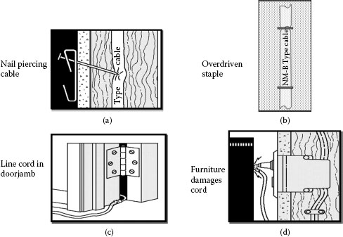
FIGURE 15.1
Examples of potentially hazardous for behind-the wall and exposed wiring (a) nail pierces behind-the-wall wire insulation, (b) over-driven wire staple, (c) cord crushed in door jamb, (d) cord pinched by furniture.

Since the late 1980s, research on mitigating residential electrical fires produced from electrical arcing faults has led to the development of the first commercially available Arc Fault Circuit Interrupter (AFCIs) in 1999 [5,6,7,8]. These circuit protection devices are designed to mitigate the effects of electrical arcing faults that are not detected by ordinary thermal-magnetic (T-M) circuit breakers or other types of circuit protection devices [5,6,7,8,9,10]. These new circuit protective devices have the potential to reduce property and equipment damage and minimize personnel injury by their ability to sense various types of arcing faults [5,6,7,8,9,10]. Today, AFCI technology is an actively researched field with many companies and universities pursuing advancements in detection methodology, testing standards, and basic arc physics to advance electrical safety [9, 11,12,13,14,15,16,17].

Because arcing fault properties are the key to the development of these protective devices, three types of fault conditions will be examined along with a basic description of how AFCI breakers operate and how wiring and loads can affect arc detection. Since residential applications are currently the only commercial application of this technology, the scope of this work covers residential applications on the basis of North American standards with some coverage on commercial and industrial arcing faults.

15.2 Arc Fault Circuit Interrupters (AFCIs)

The branch feeder (B/F) AFCI, commercially introduced in 1999, effectively lowered the magnetic instantaneous trip threshold of a thermal-magnetic (T-M) breaker from the typical range of 200A_rms to 250A_rms down to 75A_rms (as seen in Figure 15.2) while still retaining the standard thermal-magnetic overload trip features of a traditional breaker [5,8,9,10]. However, the B/F device had limitations in that it could not sense arcing faults below its detection limit of about 75A_rms.

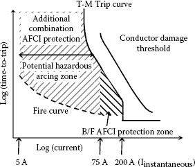
FIGURE 15.2
Additional protection zones provided by the B/F and combination breakers are indicated by the shaded areas. The fire curve is described in the following section.

The now outdated B/F device was replaced by the combination AFCI breaker which provides both branch feeder protection (i.e., behind-the-wall wiring having two wires with ground) and outlet protection (two wire cord), essentially combining both branch feeder and outlet protection, hence the name combination. A combination AFCI breaker has the ability to detect arcing faults without the need for ground fault, detecting arcing faults down to as low as 5A_rms as shown in Figure 15.2 [18,19,20,21,22].

One of the biggest challenges for designers of these devices was in the ability to discriminate between arcing faults and loads that normally arc during operation (e.g., motors, certain types of lighting, switches, etc.) and loads that have high di/dt [20]. Frequently, highly nonlinear currents with series arcing can be difficult to distinguish from the normal waveform without arcing. Figure 15.3 illustrates some examples of current waveforms from some loads which inherently produce nonsinusoidal current.

In designing AFCI breakers and other types of protective devices, the HF current from the arc is utilized [23] in algorithms, processed with microcontrollers, to identify arcing faults [18,19,20,21,22]. These algorithms generally use a combination of characteristics inherent in arcs including threshold signals obtained from broadband RF current generation produced from the arc and duration patterns. Since the focus of this section is on arcing fault phenomena, specific algorithms are not described in detail but rather can be found in the patent and nonpatent literature [18,19,20,21,22,23].

Commercially available combination AFCIs generally use a measure of the power frequency current and a bandpass filtered RF current signature to make a trip/no trip decision on the basis of proprietary algorithms [18,19,20,21,22]. A simplified block diagram of the RF sensing method is shown in Figure 15.4. Generally some means of bandpass filtering is used to only pass specific frequency range(s) of interest, consisting of one or more frequency bands. By measuring the amplitude and duration of the RF current at specific frequency band(s), a software algorithm can be used to determine if an arcing fault is present.

For currents below the instantaneous magnetic trip threshold of a breaker, decision times (i.e., time to trip) can be found in the latest UL1699 standard [24]. This standard has many requirements, including arcing tests used to determine if the AFCI device trips fast enough to meet minimum standards. One of the tests is named the carbonized path clearing time test because the test consists of creating a carbonized path or carbon bridge in SPT-2 lamp cord. This carbon path is intended to replicate the conditions formed when a broken conductor arcs while under load resulting in carbonized insulation [24]. Wire samples are prepared per the standard, by cutting the insulation across a lamp cord (SPT-2), exposing the copper wire strands and then wrapping the cut portion with electrical tape and cloth tape to replicate a repaired wire. HV is applied to the wire to create a carbonized path across the cut in the insulation, creating a wire with arcing damage. After the HV conditioning requirements have been meet, 120 Vac is applied to the wire sample at a specified current to initiate arcing. Continuous series arcing must occur for the test to be declared valid and the AFCI device must trip within a specified time per the standard [24].

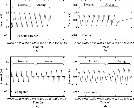
FIGURE 15.3
Illustrations showing how difficult it can be to detect series arcing faults for various nonsinusoidal loads; (a) Vacuum Cleaner; (b) Dimmer; (c) Computer; (d) Compressor.

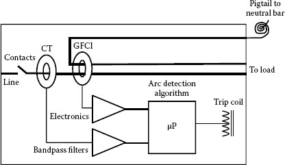
FIGURE 15.4
Block diagram showing RF current spectrum method of arc detection.

FIGURE 15.5
UL1699 “fire” curve. (Curve and circuits taken from UL Standard for Safety for Arc-Fault Interrupters, UL1699 rev. 4, Feb. 11, 2011.)

The higher the current, the faster the breaker must trip to decrease the probability of starting a fire owing to the higher arc energy. It has been shown that the probability of igniting a fire under these conditions increases with increased arcing current [24]. On the basis of experimental data, a “fire” curve (Figure 15.5) was developed that indicates the maximum allowable time for AFCI device trip as a function of the power line current. This test requires that the arcing fault be located in various positions in the circuit (configurations A, B, C, D), representing the different locations an arcing fault can occur in a branch circuit [24].

Another test, called the opposing electrode test, consists of an arc generator (with copper and graphite electrodes), a resistive load R, and a masking load (configuration A, B, C, or D). There is no masking load used in configuration A. Like the carbonized path clearing time test, the AFCI device in this test must also trip within the allowed time indicated by the “fire” curve (i.e., below the fire curve).

15.3 Arcing Faults

It is generally considered that there are three classifications of arcing faults in residential circuits: short-circuits (i.e., parallel arcs), broken conductors/wire (i.e., series arcs), and loose overheated connections (i.e., glowing connections). Per UL1699, AFCI devices are intended to detect and trip within the required time on short-circuit and series arcs above 5A_rms. They are not intended to detect glowing connections although it is recognized that a glowing connection may progress into a series arc which may be detected [25].

To illustrate the differences in faults, Figure 15.6 compares the three types of fault conditions that can occur in a residential electric circuit—short-circuit (overheated extension cord under a rug), series arc (broken conductor inside an appliance cord), and glowing connection (loose wirenut) and corresponding waveform examples.

FIGURE 15.6
Photographs of three types of residential faults and associated waveforms; (a) Parallel arcing; (b) Series arcing; (c) Glowing connection [27,37,38].

15.3.1 Short-Circuit Arcing

The stranded wire lamp cord (e.g., SPT-2) used in many extension cords, lamps, and appliances can become cut, crushed, pinched, over-heated, or deteriorated from old age exposing the metal conductors. Exposed live wires can create line-to-neutral or line-to-ground arcing faults, defined as a short-circuit arcing fault. The UL1699 standard refers to a guillotine test for measuring the high current arcing performance of an AFCI device [24].

In residential applications a short-circuit arcing fault is commonly referred to as a “parallel” arc fault. This “parallel” short-circuit arc generally produces a high current fault with a magnitude that depends on the available short-circuit current. This available short-circuit current is determined by available current at the load center and impedance of the circuit created by the fault location. Frequently, parallel faults can occur at the load which is connected by long lengths of lamp cord plus long lengths of “behind-the-wall” cabling (i.e., typically NM-B) cable length as illustrated in Figure 15.7. The longer these wires and the smaller their conductor size, the greater the impedance and the lower the available fault current becomes at the load.

It was recognized that a home fire could be initiated by a continuous short-circuit with a low available fault current [1,2]. It was also discovered that intermittent arcing can occur with a low available fault current, also called a sputtering arc [5,9]. Frequently, sputtering arcs are created by damaged stranded extension or lamp cords owing to the fine wire strands of the lamp (or appliance) cord (e.g., SPT-2) vaporizing [1,12,26]. The strands intermittently make and break creating sporadic arcing, carbonizing the wire insulation, which may not activate the thermal overload (i.e., bimetal) of a standard breaker to trip the breaker. This type of arcing fault can persist and create a hazardous condition, producing hot molten copper particles that get violently ejected from the fault along with ignited gasses and a hot arc, possibly igniting a fire. Consequently, a standard T-M breaker may not trip or trip after significant arcing has occurred, greatly increasing the probability of igniting a fire in either the wire insulation or in the surrounding material [27].

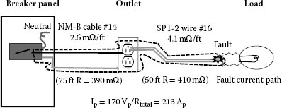
FIGURE 15.7
Drawing illustrates typical wiring setup in residential North American applications. This example shows how the available short-circuit current can be below the instantaneous pickup level of a traditional T-M breaker.

Another form of parallel arcing can occur by “scintillation” [28,29,30]. Scintillations start as small, very low current, partial breakdown between two conductors at different potentials, across an insulating surface [26, 28,29,30]. Repeated breakdown can lead to carbonization of the surface (i.e., carbon bridge formation) and potentially a parallel arcing fault [28,29,30]. It is also known that old wiring will deteriorate and can be prone to arcing faults [31].

15.3.2 Series Arcing

Figure 15.6b shows how a broken wire in one conductor leg of a hair dryer cord created a series arc. A low current arcing fault, often referred to as a “series” arc fault because the arc fault is initially in series with a load, is an unintended arc created by either a break in the line side or neutral conductor. This section shows how continuous low current arcing can occur at residential voltage levels (i.e., 120V_rms) and illustrates some examples of low current “series” arcing faults.

If one were to examine the Paschen breakdown curve for air at atmospheric pressure (see Figures 9.8 and 15.9) the lowest possible breakdown voltage. is around 327V [32,33,34,35]. This implies that for continuous arcing, the voltage must be greater than this value, otherwise the arc will extinguish at the first half-cycle zero crossing. It is possible for extremely small contact gaps that breakdown of the gap can occur for much lower voltages, see Section 9.3.2. Usually, however, when a 120V_rms circuit with two copper wires conducting current is pulled apart, even with a small gap, the arc extinguishes in ½ cycle. So, how does a series break in a conductor of a circuit operating at 120V_rms (170V_p) produce continuous “series” arcing at voltages below the Paschen minimum for air at atmospheric pressure? It turns out that in general, virtually all residential wiring and distribution equipment (i.e., outlets, fixtures, etc.) use some type of organic material (e.g., polyvinyl chloride [PVC], nylon or other types of thermoplastic materials) to insulate conductors. If this insulation is exposed to intermittent arcing or elevated temperatures, say from a loose connection, it can decompose and produce carbonaceous material (i.e., long chain hydrocarbons) [28,29,30,34]. This carbon is the reason why sustained “series” arcing is possible at 120V_rms. Carbon is an excellent thermionic emitter (see Figure 15.9) with a very high vaporization temperature [31,32,33,34,35]. If a connection arcs intermittently or a broken wire occurs creating a series arc, the wire or nearby insulation can become carbonized, coating the copper wire surface and even creating a carbon bridge across the gap formed by the break in the conductor [29, 33]. Now rather than a pure copper wire, the wire acts like more like a carbon electrode and carbon electrodes, even at low currents, can sustain arcing since carbon is an excellent thermionic emitter with a negative temperature coefficient [32,33,35].

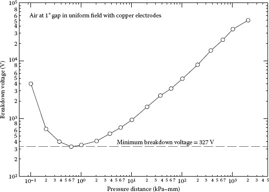
FIGURE 15.8
Paschen curve for air. Note minimum breakdown is 327V making 120V_rms (170V_p) seem too low for continuous arcing.

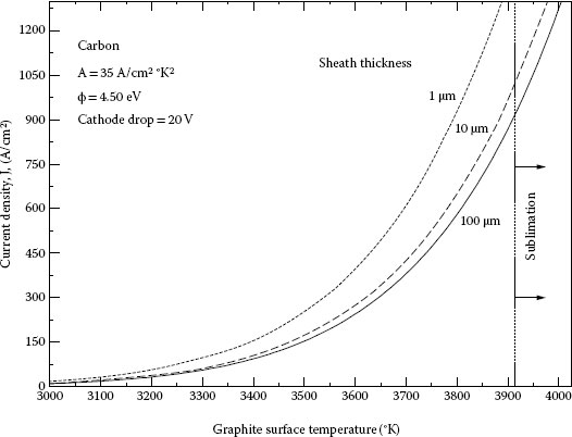
FIGURE 15.9
Thermionic emission for graphite [36].

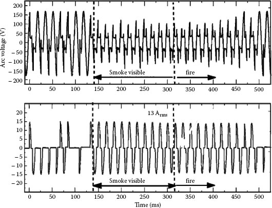
FIGURE 15.10
Arcing in SPT-2 cord at 13 A_rms initiated fire after 316 ms of arcing. Line-to-neutral arcing eventually occurred after the wire insulation burned through to both conductors at 6.7s [27].

Once the carbon becomes heated from the arc, its thermionic emission and negative temperature coefficient properties result in continuous “series” arcing faults. Once either a carbon bridge is formed or carbon coats the conductors in a broken connection, continuous arcing at 120V_rms becomes possible as shown in Figure 15.10 [27].

To ignite a fire, the arc needs to have a fuel source. Many times, the wire insulation itself becomes the fuel source, especially PVC insulation which can produce volatile gasses that can be ignited by the arc [37,27,28,29,30,34]. Gas ignition, not the arc itself, is generally observed during an arcing event since the chemical energy released from the burning gasses is far greater than the arc energy [37]. It is the ignited gases which can subsequently ignite surrounding materials such as structural wooden members, rugs, newspapers, or other materials and generally not the arc itself [37,27,28,29,30,34].

15.4 Glowing Connections

A third type of electrical fault that can occur in residential electrical systems is frequently referred to as a glowing connection (Figure 15.6c, see also Section 6.4.3.3) [38]. Glowing connections are molten metal and metal oxides that generally occur at a loose connection point in an electrical circuit [38,28]. The molten metal/oxide can reach temperatures around 1235°C (melting point of Cu₂O) [39–40]; well above the melting and vaporization temperature of polymeric insulation used in wiring [30,34,41]. Depending on current magnitude, 10s of watts of power can be dissipated in the loose joint causing overheating of electrical wiring and the surround area [38]. These very high temperatures at the connection interface can propagate down the conductor to the wire insulation and the surrounding structure (i.e., outlet housing or wood framing), leading to charring of the insulation and wood and potential ignition of the wire insulation, plastic outlets, wood framing, etc. [30]. While a glowing connection is technically not an arc, it does have characteristics similar to a plasma owing to its high temperature [42]. Its presence goes undetected by present day AFCIs [24]. However, it has been shown that fires can be prevented owing to a glowing connection because in some cases the glowing connection will progress to an arcing fault which can be detected by an AFCI device [25].

Frequently, a glowing connection can be a slowly progressing phenomenon, generally associated with loose electrical connections, worn out connections, applications involving vibration, or poorly designed connections [34,42,43,44,45]. Glowing connections have been documented in residential AC circuit (i.e., 120V_rms in North America, 220V_rms in Europe, 100V_rms in Japan) [29,45,48].

Glowing connections were initially studied in the mid 1970s in Japan [47,48] and then at the National Bureau of Standards (NBS) (now the National Institute of Standards (NIST)) in the late 1970s [49]. Others have also documented glowing connections [50,51]. Japanese researchers and a few researchers in the US showed some images of glowing connections and documented their effects on electrical safety [38,34,48]. Aronstein has also documented practical examples of safety hazards from glowing connections in wire nuts and especially the hazards associated with improperly installed aluminum wiring [52,53].

The ability of a glowing connection to be self-sustaining has been previously documented but detailed measurements on the characteristics and physics of this phenomena have not been documented under controlled conditions until recently [38,39,42].

Glowing connections can form at the interface of an electrical connection and are characterized by an incandescent orange glow of molten oxide [38,34,45]. Usually, the glowing connection would be the unintended result of a loose connection that intermittently arcs under load current. Depending on the connection material, it may take thousands of make/break arcing cycles and just the proper alignment of the wires to make a glow occur [38, 30]. In other materials, especially ferrous materials, the glow can occur with only a few or as little as one make/break operation under load [27]. Repeated make/break action of a loose connection is generally a precursor for the initiation of a glowing connection because the arc creates a metal oxide on the connection interface [38,30,39,40]. These semi-conductive oxides can form a resistive interface that can lead to glow formation [38,30,39,40]. Due to surface tension, it is suspected that the repeated make/break arcing action draws a thin strand of metal/metal oxide, heated to high temperatures owing to the high current density [38,39]. With sufficient oxide present on the surface of the interface, the glow will be initiated and sustained owing to the negative temperature coefficient of resistance of the metal oxide (e.g., Cu₂O, CuO). The glow can continue to consume the metal wire (i.e., convert metal to metal oxide) for extended periods of time (up to hours) [38,34]. The material type and current level also determine the type and stability of the glow.

The glowing phenomenon is not to be confused with I²R resistive heating created from inherent connection resistance. Figure 15.11 illustrates how glowing connections can form in a loose or broken electrical connection. A “good” connection has a low resistance interface at the connection point along with a low mV drop and low and stable connection temperature. A loose connection can arc under load and create metal-oxide at the connection interface. The voltage drop across the connection will increase, intermittent short duration arcing may occur, along with an increase in the interface temperature. Even without arcing, millivolt drops may exceed softening temperatures and approach melting temperatures of the connection metals (see Lorenz voltage-temperature properties). A glowing connection can form if the metal-oxide at the connection interface becomes heated to the molten state [39]. This heating can be caused by a high-current density created by a thin strand of metal oxide being drawn between the interface or if the joule heating of the metal oxide is high enough to melt the oxide then a glow will form [38,39]. The glow can be modeled as a molten metal-oxide in parallel with a solid metal-oxide with voltage drops of about 2 to 10V_rms (depending on current and materials) and very high and rising connection interface temperatures [38,39].

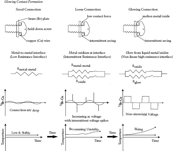
FIGURE 15.11
Conceptual sketches show the glowing connection formation process.

A device, consisting of a micrometer and a spring loaded wire holder, was designed to easily reproduce glowing connections to allow for controlled study of this phenomenon [34]. A series of photographs were taken, using this device that shows the progression of the glow over time (Figure 15.12).

An example of electrical waveforms, seen in Figure 15.13, illustrates the electrical characteristics of a copper-to-copper wire glowing connection at 2.9_Arms. The voltage waveform is obviously distorted and high in magnitude (~6Vrms), about 1,000 times higher, as compared to a good electrical connection (typically for residential electrical connections 1 to 20mΩ)! Also, the glowing voltage is well above the reported values for softening (140mV) and melting voltages (430mV) for copper. The glow is actually modulated by the ac current as seen in Figure 15.13. The molten metal-oxide filament can be seen meandering across the solid oxide bridge surface of Figure 15.12 as it is modulated on-and-off by the ac current. At lower currents (i.e., about <6Arms) the glow extinguishes near current zero because the molten-metal oxide temperature drops. The current then flows through the solid oxide bridge. On the next half-cycle, as the current magnitude increases, the solid the glow reignites. At higher currents, the glow does not extinguish at current-zero because the molten-metal oxide temperature remains high enough to maintain the metal-oxide in a liquid state [38].

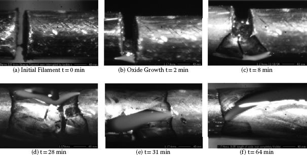
FIGURE 15.12
A time lapse series of photographs showing the initial bridge formation and growth of a glowing connection (color images show orange filament) between two copper wires. Dark area (copper oxide) 1-mm diameter wires, 37× magnification at 1.17 A_rms [34].

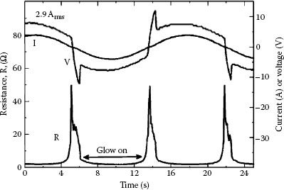
FIGURE 15.13
Dynamic resistance of glowing contact (2.9 A_rms, 1-mm diameter copper wire) shows large increase in resistance near current zero [38].

Glow voltage is a function of current. An average glowing contact voltage was measured at seven different current levels, at the time the glowing was initiated, to determine the average power dissipated in the connection as a function of current (Figure 15.14). As the current is increased from 0.9 A_rms to 5 A_rms, power dissipated at the connection interface increased from 7W to 25W and remained fairly constant at 25W to about 16A_rms. At this point the wattage rapidly increased to 50W at 20A_rms. A voltage minimum is seen near 13A_rms and increases for both higher and lower currents. Thus, with increasing current, glowing voltage actually decreases but the power dissipated in the joint increases exponentially as shown [38]. The glow voltage is well below minimum arc voltage for copper (12V) indicating that the glow is not an arc [38,39].

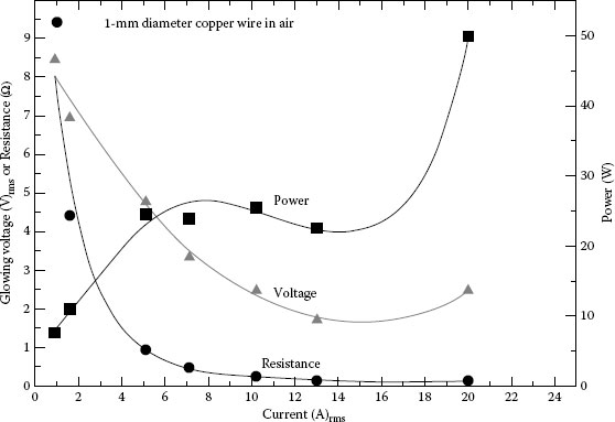
FIGURE 15.14
Typical average glowing contact voltage and power dissipated in contact for 1-mm diameter copper wire pair. Measurements taken just after glowing contact formation stabilized [38,39].

Glowing connections are expected to occur in virtually any type of electrical circuit [38,39]. Glow initiation and sustainability depend on many factors including: current, wire interface shape, wire diameter, dc or ac, and wire material [38]. Glowing connections have been created with currents as low as 250mA_rms [38].

Glowing contacts have been studied for copper conductors but there are also other materials that may be present in electrical wiring that can glow. The metals in Figure 15.15 were chosen on the basis of their potential use in various types of electrical products, copper being the most common along with steel. Alloys of copper, brass, and phosphorous bronze are used in wall outlets and electrical switches. Steels, while not intended as a conductor path, can be found in outlet screws that secure the wires in wall receptacles, junction boxes, support structures, and conduit. Sometimes the steel screws are brass or nickel plated for polarity identification purposes. However, if arcing occurs, the plating can be removed exposing the base metal (often times steel). Wire nuts also frequently use tin plated steel springs to secure conductors and can result in glowing connections [38,28,29,30,31,39,40,41,42,43,44,45,46,47,48,49,50,51,52,53].

Research has shown that the material or combination of materials affects the glowing connection voltage wave-shape and thus the power dissipated in the glowing connection [38]. Figures 15.15 and 15.16 show the very dramatic difference in voltage waveform shape for various material combinations. And, for the same combinations, Figure 15.16 illustrates how the voltage wave-shape changes at a higher current. At higher current levels, the voltage distortion tends to decrease and become more sinusoidal owing to elevated temperatures (see prior explanation in Figure 15.13).

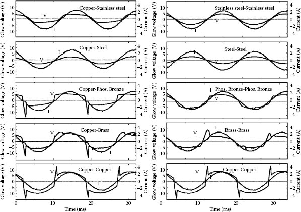
FIGURE 15.15
Current and voltage waveforms for the various material combinations all at 1.6 A_rms. All wires were 1.0 mm in diameter [38].

Figure 15.17 illustrates this material-current effect by showing the rms voltage across the glowing connection as a function of rms current for a number of different materials at 60Hz. Figure 15.18 shows the corresponding power dissipated.

The propensity of a material or material combination to begin glowing is an important measure since it reflects the probability of initiating a glowing connection which may lead to a fire. The relative ease to initiate glowing, for a given material pair, is indicated qualitatively in Table 15.1 (i.e., easy, very hard, etc.). This represents the number of make/break operations necessary to start a glowing connection. The lower the number of make/break to initiate a glow, in general, the easier it is to initiate a glowing connection.

The extinction current, in Table 15.1, shows the minimum current for existence of the glow in a steady state under the stated conditions. The minimum current to initiate glowing is considered to be about 0.25 A_rms for a brass-iron combination [38]. The outcome is a qualitative measure of how the oxide grows. Figure 15.12 shows how copper wires are consumed and form copper-oxides along the wire lengthwise. Slow growth, such as in case of an iron based wire, indicates that glowing occurs at the interface rather than over a distinct molten filament on the oxide surface as in the copper-to-copper case seen in Figure 15.12. Material properties of commonly used metals for electrical application are shown in Table 15.2.

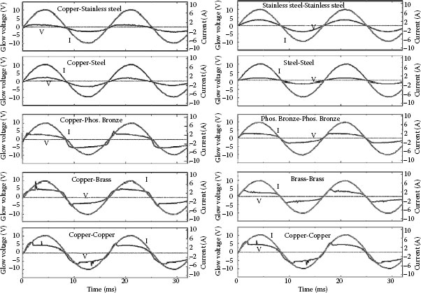
FIGURE 15.16
Current and voltage waveforms for the various material combinations all at 5 A_rms. All wires were 1.0 mm in diameter [38].

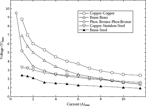
FIGURE 15.17
The true rms voltage as a function of current for the various combinations of wire materials at 60Hz. Except for the iron based materials there is an exponential decrease in voltage with increasing current [38].

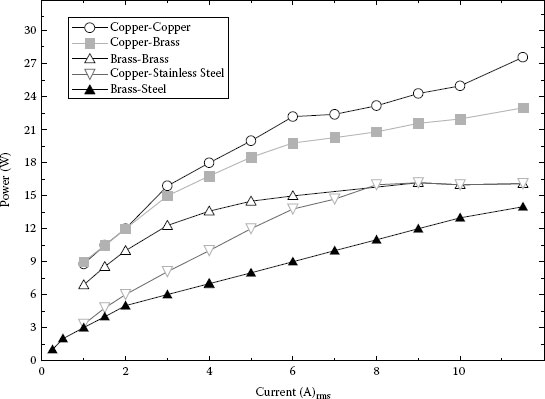
FIGURE 15.18
Power dissipated in the glowing connection as a function of current for various material combinations at 60Hz [38].

TABLE 15.1
Wire Materials Combinations and Outcomes

Material Type	Extinction Current (Ar_ms)	Outcome	Possible Oxide Products	Ease to Initiate Glow
Copper – Copper	1.0	Breeding	Cu₂O, CuO	Hard
Brass – Brass	1.0	Slow Growth	Cu₂O, CuO, ZnO	Hard
Steel – Steel	1.0	Slow Growth	FeO, Fe₂O₃, Fe₃O₄	Very Easy
Stainless Steel – Stainless Steel	0.5	Slow Growth	Cr₂O₃, NiO, FeO, Fe₂O₃,Fe₃O₄	Very Easy
Phosphor Bronze – Phosphor Bronze	0.5	Breeding	Cu₂O, CuO, SnO₂, Sn₂O₄	Very Hard
Copper – Brass	1.0	Breeding	Cu₂O, CuO, ZnO	Hard
Copper – Phosphor Bronze	1.0	Breeding	Cu₂O, CuO, SnO₂, Sn₂O₄	Very Hard
Copper – Steel	1.0	Slow Growth	Cu₂O, CuO, FeO, Fe₂O₃, Fe₃O₄	Easy
Copper – Stainless Steel	0.5	Slow Growth	Cu₂O, CuO, FeO, Fe₂O₃, Fe₃O₄, Cr₂O₃, NiO	Easy

All wires 1.0-mm diameter. Degree of ease to initiate glow scale: Very Easy = 1 to 2, Easy = 2 to 10, Hard = hundreds, Very Hard = hundreds to thousands of make/break operations [38].

TABLE 15.2
Wire Material Properties

Material Type	Composition (wt%)	Metal MP (°C)	λ (W/m°K)	Melting Point (MP) of Various Stable Oxides (°C)
Copper	Cu (99.999)	1083	400	1235 (Cu₂O) and 1326 (CuO)
Brass 260	Cu/Zn (70/30)	915–955	109	1975 (ZnO) + copper oxides
Steel 1006	Fe/C/Mn (99.5/0.06/0.35)	1535 (Fe)	46	1457 (Fe₂O₃), 1597 (Fe₃O₄), 1360–1424 (FeO)
Stainless Stee 302	Fe/Cr/Ni/Mn (71./18/8/2)	1400–1420	16	2400 (Cr₂O₃) and 1984 (NiO) + steel oxides
Phosphor Bronze 510	Cu/Sn/P(94.8/5.0/0.2)	975–1060	84	540 (SnO2) and 1100d. (Sn₂O₄) + copper oxides

All wires 1.0-mm diameter. Steel 1006 (Fe/C/Mn/P/S) (99.5/0.06/0.35/0.04/0.05). Stainless steel 302 (Fe/Cr/Ni/Mn/Si/C/P/S) (71./18/8/2/0.75/0.15/0.04/0.03). Potential intermetallic oxides are not listed. (d. Decomposes, thermal conductivity, λ, given at 20°C) [38].

15.5 Arcing Fault Properties

AFCI breaker designers utilize the fact that arcing faults produce broadband RF currents [54,55,56,57,58,59]. Since many loads can produce RF current during normal operation, one of the greatest challenges in developing AFCI technology is the ability to distinguish between loads that produce RF currents and undesired arcing faults [20]. This is so difficult because many loads either arc or mimic arcing during normal operation. For example, arcing can occur in a light switch operated under load and, commutation brushes of a motor while high frequency noise, that mimics arcing, can occur in high intensity discharge lamps and compact fluorescent lamps. Various algorithms, using RF current magnitude and duration, pattern recognition, and frequency bandwidth, have been developed for distinguishing “good” intentional arcing (or electronics that create HF signals) from ‘bad” or unintentional arcing [18,19,20,21,22,23]. Furthermore, there are many other factors that can influence the RF current signal generated by an arc fault (or HF produced from electronics). The main factors being the frequency range of interest, arcing current magnitude, cable and circuit influences, and arc gap materials. The following sections examine each of these factors to illustrate how they affect the magnitude of the RF current generated by the arc fault as seen by an AFCI protective device.

15.5.1 Frequency

It is well documented that broadband RF current can be generated by an arcing fault [54,55,56,57,58,59]. One example of the spectral output of a 5A_rms arcing fault over a 20MHz bandwidth is shown in Figure 15.19. Notice how the amplitude generally decreases across the frequency range shown. This data shows the level of detection circuit sensitivity needed to detect arcing in this particular circuit. There are situations where a load (e.g., inverters, compact fluorescent lights, or motors, etc.) may produce high harmonic content at a frequency used by the AFCI device [14,16,20]. Also, power-line carrier signals can operate in the 100kHz range and other smart grid devices can produce high frequency signals on a residential circuit that must be tolerated by the AFCI device. To prevent false tripping, AFCI devices generally utilize more than one frequency or operate over a broad range of frequencies to reduce false tripping [18,19,20,21,22,23]. Also, because there is generally a high background noise in many ac power systems below 2.5kHz as seen by the dramatic rise in RF voltage shown in Figure 15.19, many designs tend to use a frequency range above this level [18,19,20,21,22,23]. The upper frequency limit is generally limited by transmission line effects combined with a diminishing signal and more costly electronics, making the useful detection range between about 2.5kHz to 20MHz [18,19,20,21,22,23,33].

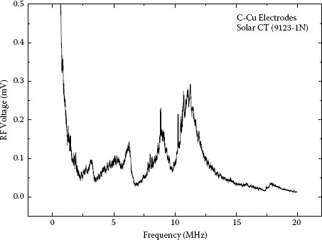
FIGURE 15.19
Spectrum analyzer output of a 5A_rms series arc illustrating the RF signal magnitude over DC to 20MHz bandwidth. Voltage input to spectrum analyzer shown (50 Ω load). Results not compensated for CT probe frequency response.

15.5.2 Electrode Materials

The type of material that create the anode and cathode of an arcing fault gap also have an effect on the RF current generation. It has been shown that very little RF current is produced from carbon electrodes and high RF currents are generated from copper and other nonthermionic metals with RF current being produced from the cathode since it is an electron source [33,36]. The RF current generation is attributed to arc root instabilities on the cathode caused by an inherent high current density of the arc root on nonthermionic emitting material (i.e., copper) [36,60]. The arc voltage waveforms of Figure 15.20 illustrates an example of this instability in arc voltage for Cu-Cu (nonthermionic) electrodes as compared to a much smoother arc voltage for C-C (thermionic) electrodes. Figure 15.21, a real-time spectrum analyzer (RSA) output for a 2.5A_rms series arc created with the opposing electrode arc generator [24], with Cu-C electrodes, clearly illustrates this effect, with RF current generated from the cathode. The highest amount of RF current is produced when the cathode is made from a nonthermionic emitting material (e.g., copper). Very little RF current is produced from a graphite cathode except at very low currents [33,36]. Fortunately, virtually all residential wiring is made of nonthermionic materials (i.e., Cu), but significant amounts of carbon, produced from burned insulation, may reduce RF current generation or become intermittent and make arc detection more difficult in some situations.

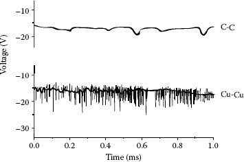
FIGURE 15.20
Expanded views of the arc voltage during a portion of a 60Hz half cycle that shows the difference in HF arc voltage activity between copper and carbon electrodes at 4.5A_rms [36].

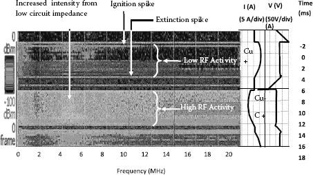
FIGURE 15.21
Real-time spectrum analyzer (RSA) output shows broadband RF current is predominantly produced when the cathode is made from a nonthermionic emitting material (copper) (4.8A_rms at 120Vac copper-graphite electrodes in the opposing electrode arc generator) [33].

15.5.3 Arc Fault Current

The magnitude of the power frequency current (i.e., 60Hz) also has a significant effect on the magnitude of the RF current generated by an arc fault [33]. Generally, the lower the arcing current, the greater the RF current magnitude generated and the easier it is to detect with an AFCI device. Conversely, it was discovered that the amplitude of the RF current signal decreases with increasing arc current [33]. Above about 30A_rms there is a significant drop-off in the measured RF current as shown in Figure 15.22. This can be very significant effect for designers of AFCI protective devices since it may not be possible to use RF current sensing methods at high arcing currents [33]. Oftentimes, the only RF current is produced at the current zero crossings in ac systems.

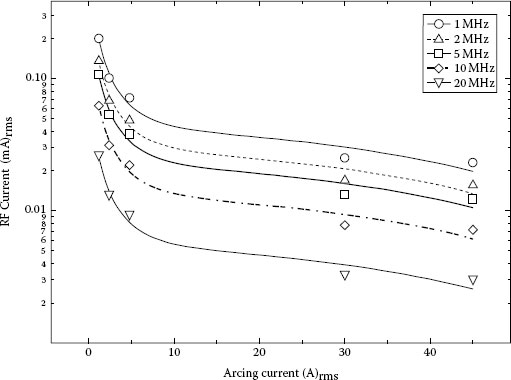
FIGURE 15.22
RF current produced by series arcing faults (copper–graphite opposing electrodes) at 120Vac for different arcing fault currents. RF current generally decreases in magnitude with increasing arcing current and increasing frequency.

15.5.4 Cable Impedance and Cable Length Effects

RF current, circulating through household wiring and through an AFCI device, can be greatly affected by the circuit impedance [14,33,61]. Wire capacitance and inductance affect the RF current magnitude, especially at higher frequencies. In particular, discrete shunt capacitance across the load or along the branch circuit, from loads in other upstream outlets, can have a significant effect on the magnitude of the RF current “seen” by the AFCI device.

The circuit impedance in a residential branch circuit depends on cable type, length, load, and source impedance. Since many AFCI devices operate in the MHz range, cabling can act like a transmission line—creating standing waves with varying levels of RF current magnitude along the cable’s length causing the level of RF current at the AFCI device to depend on cable properties and length [33,61].

At the RF frequencies of interest, residential wiring can act like a transmission line with the impedance, Z_b, as seen by the protective device, can be represented by Equation 15.1.

$Z_{b} = Z_{0} \frac{Z_{L} + j Z_{0} T a n (β l)}{Z_{0} + j Z_{L} T a n (β l)}$ $Z_{b} = Z_{0} \frac{Z_{L} + j Z_{0} T a n (β l)}{Z_{0} + j Z_{L} T a n (β l)}$

(15.1)

$β = \frac{2 π}{λ}$ $β = \frac{2 π}{λ}$

(15.2)

where Z_o is the wire’s characteristic impedance given by

$Z_{0} = \sqrt{\frac{R + j ω L}{G + j ω C}}$ $Z_{0} = \sqrt{\frac{R + j ω L}{G + j ω C}}$

(15.3)

and λ the wavelength of the RF current and Z_L the magnitude of the load impedance.

Equation 15.3 can be simplified with a lossless case (i.e., R = 0 wire series resistance and G = 0 line-to-line wire conductance) resulting in the following:

$Z_{0} = \sqrt{\frac{L}{C}}$ $Z_{0} = \sqrt{\frac{L}{C}}$

(15.4)

Typical values for commonly used residential wiring are shown in Tables 15.3 and 15.4. Cable length can also affect the magnitude of the RF current seen at a protective device. With longer cable lengths (Figure 15.23), the cable can become multiple wavelengths long (λ = c/f), especially at higher frequencies, creating multiple impedance peaks and valleys (Equation 15.1) along the cable resulting in varying levels of RF current magnitude along the cable length.

The wave propagation speed, v, is a measure of how fast a signal travels through a media. A radio signal in free space travels at the speed of light, c, approximately 3 × 10⁸m/s, but a signal on a transmission line (e.g., NM-B cable at high frequencies) travels slower compared to the speed of light, effectively increasing the electrical line length. In twisted pair wires and NM-B type cable, the velocity of propagation may be 40% to 75% of the velocity in free space [61,62]. The relationship between propagation velocity v, and the speed of light is given by

$v = cVF$ $v = cVF$

(15.5)

TABLE 15.3
Electrical Properties of Various Types of Commonly Used Residential Wire

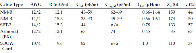
All values taken at 100kHz. Resistance is per wire conductor, Differential capacitance (line-line (L-L)), is measured between conductors, L is measured as loop inductance of the line-line conductors. Zo and VF are calculated using equations 15.4 and 15.7, respectively, using median values for CL-L and LL-L. NM-B has 2 conductors plus a bare ground wire. SPT-2 is 2 conductor PVC lamp/appliance cord. BX is 4 insulated conductors in a steel sheath.

TABLE 15.4
Dielectric Properties of Various Types of Insulation Used in Electrical Products

Insulation	ε_r	$VF = \frac{1}{\sqrt{ε_{r}}} (%)$ $VF = \frac{1}{\sqrt{ε_{r}}} (%)$
PVC	4.0	50
Nylon	3.7	52
HDPE	2.7	60
Polypropylene	2.3	66
Polycarbonate	4.4*	49

(at 60Hz unless otherwise noted) * 1kHz [61,62].

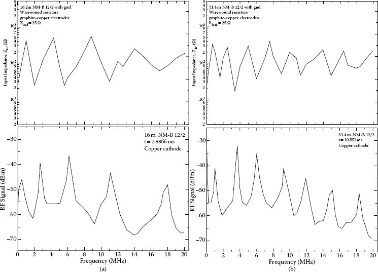
FIGURE 15.23
Change in cable length translates into a change in RF current magnitude versus frequency due to an approximate doubling of the wave propagation time from reflections from the load. Increased RF signal corresponds to low impedance (i.e. valley in input impedance). Velocity factor, VF, remains equal in both cases since the same cable was used in both cases. (NM-B 12/2 cable) (a) 16.2m and (b) 31.4m [33].

where VF is written as

$VF = \frac{1}{\sqrt{ε_{r}}}$ $VF = \frac{1}{\sqrt{ε_{r}}}$

(15.6)

or for the lossless case

$VF = \frac{1}{c \sqrt{L C}}$ $VF = \frac{1}{c \sqrt{L C}}$

(15.7)

where ε_r is the relative permittivity of the cable insulation and L is wire inductance per unit length and C the wire capacitance per unit length. The velocity factor, VF, is a percentage of the speed of light, c, and for wire insulation made from PVC, the wave propagation velocity is approximately 50% that of the speed of light in free space. Meaning that for a given frequency, the wavelength is half as long as compared to the wavelength in free space making a given cable length effectively double as compared to the wave traveling at the speed of light. Knowing either the relative permittivity of the cable insulation or the L and C per unit length of the cable will allow for calculating VF.

Thus, for a given frequency, the magnitude of the RF current depends not only on the cable properties but also on the cable length and the location along the cable where the RF current is measured. The greater the circuit impedance at a given frequency, the lower the RF current and, conversely, the RF current magnitude will be higher at impedance valleys. This effect can be very significant since an AFCI protective device is expected to function properly for any cable length. There are many books and references on transmission line theory which the reader can refer for further study [61].

15.6 Other Types of Arcing Faults

While there is certainly much interest in residential arcing faults that may lead to fires, other applications such as commercial and industrial cover a wide range of circuits, currents, and voltages, especially 240Vac and higher [63,64,65,66]. Fault conditions that can occur in residential applications (i.e., series, parallel, and glowing) can also occur in commercial and industrial settings as well, but generally lead to arcing faults that can produce not only electrical fires but also produce significant arc flash which can cause serious injury or even death [67,68,69,70,71,72,73]. Accidents include series arcing that can progress to parallel arcing (line-to-line or line-to-ground), accidentally shorting a live conductor, animal shorting out live conductors, loose connections, degraded and/or contaminated insulation, especially at medium voltages [69]. Many of these problems can result in a large energy arc flash that can cause serious burns and even death to personnel near the arc flash zone and/or cause serious equipment damage [69]. A number of solutions used today to mitigate the effects of an arc flash include: protective clothing, crowbar devices that sense arcing faults and extinguish the arc flash in milliseconds, maintenance mode switches that reduce the trip time of a breaker when maintenance is being performed on a live circuit, zone selective interlocking (ZSI) (a method which allows two or more ground fault breakers to communicate with each other so that a short-circuit fault or ground fault will be cleared by the breaker closest to the fault in the minimum time), and fast shunt and arc flash energy diverters [66,67,68,69]. However, there is much room for improvement and new innovation to help further reduce the number and severity of injuries that occur each year.

15.7 Conclusions

Arcing faults can be effectively detected by AFCI protective devices. They effectively extend the protection level down to 5 Amps by responding to both sputtering arcing faults and low current “series” arcing faults. Both low current (series) and short-circuit (parallel) arcing faults can be reliably detected and discriminated from loads that inherently arc and loads that mimic arcing faults making AFCI technology a very reliable form of arc fault detection in residential applications. Many arcing fault properties have been discussed along with their effect on arc fault detection. AFCI technology, combined with continuous improvements in connection methods, insulation materials, installation standards, and insulation monitoring are all needed to further reduce electrical fires and enhance electrical safety. Continued study of arcing fault phenomena will also lead to new insights and developments.

References

1. L . Smith and D McCoskrie, “Residential Electrical Distribution Fires,” US Consumer Product Safety Commission Report, Dec. 1987.

2. J . Mah, L Smith, and K Ault, “1997 Residential Fire Loss Estimates,” CPSC Tech. Report, 1997, Available at www.cpsc.gov/LIBRARY/fire97.pdf.

3. J .R Hall, Jr., Home Structure Fires Involving Electrical Distribution or Lighting Equipment, NFPA, 1 Batterymarch park, Quincy, M.A .02169-7471, March 2008.

4. R .esidential Building Electrical Fires, TFRS, US Fire Administration National Fire Data Center, Vol. 8, Issue 2, March 2008.

5. C . Kimblin, J Engel, and R Clarey, “Arc-Fault Circuit Interrupters,” IAEI, Illinois July 2000.

6. National Electric Code (NEC), National Fire Protection Association (NFPA) 70, 1 Batterymarch Park, Quincy MA, 02169-7471 1999.

7. P . Boden, R Davidson, W Skuggevig, R Wagner, adn D Dini “Technology for Detecting and Monitoring Conditions That Could Cause Electrical Wiring System Fires,” Prepared for U.S .Consumer Product Safety Commission by Underwriters Laboratories Inc., Contract No. CPSC-C-94-1112, Sept. 1995.

8. “Report of Research on Arc-Fault Detection Circuit Breakers for National Electrical Manufacturers Association,” U.L .Project Number 95NK6832, March 1996.

9. R .W MacKenzie and J.C .Engel, “Electronic Circuit Breaker with Protection Against Sputtering Arc Faults and Ground Faults,” US. Patent# 5,224,006 29 June 1993.

10. J .C Engel and R.W .MacKenzie, “Low Cost Apparatus for Detecting Arcing Faults and Circuit Breaker Incorporating Same,” US. Patent# 5,691,869 25 Nov. 1997.

11. J .A Wafer, “The Evolution of Arc Fault Protection in Residential Systems,” Mort Antler Lecture at the 51^st IEEE Holm Conference, Chicago, IL, Sept. 2005, www.ewh.ieee.org/soc/cpmt/tc1/h2005wafer.pdf.

12. U .nderwriters Laboratories Inc. (UL). U.L .Standard for Safety for Arc-Fault Interrupters, U.L .1699, Northbrook, I.L .60062-2096 Feb. 26, 1999.

13. E . Carovou, J.B.A. Mitchell, N Ben Jemma, S Tian, and H Belhaja, “AC Electrical Arcs with Graphite Electrodes,” 57^th IEEE Holm Conference, Minneapolis, M.N .pp. 232–237, Sept. 2011.

14. P . Muller, S Tenbohlen, R Maier, and M Anheuser, “Influence of Capacitive and Inductive Loads on the Detectability of Arc Faults,” 57^th IEEE Holm Conference, Minneapolis, M.N .pp. 143–148, Sept. 2011.

15. J .-M. Martel, M Anheuser, and F Berger, “A Study of Arcing Fault in the Low Voltage Electrical System,” 25^th International Conference on Electrical Contacts with 56th IEEE Holm Conference, Charleston, S.C .pp. 199–209, Oct. 2010.

16. C Strobel “Arc Fault Detection in A.C .and D.C .Systems,” Proc. 21^st Albert-Keil-Kontaktseminar, Karlsruhe, Germany, Sept. 2011.

17. J .M Martel, M Anheuser, and A Hueber “Protection Against Parallel Arcing in Residential Installations,” Proc. 21^st Albert-Keil-Kontaktseminar, Karlsruhe, Germany, Sept. 2011.

18. K .L Parker and T.J .Miller “Arc Fault Circuit Interrupter And Method Providing Improved Nuisance Trip Rejection,” U.S .Patent #8,089,737 Jan. 3, 2012.

19. X . Zhou, J.J .Shea, J.C .Engel, K.L .Parker, and T.J .Miller “Arc Fault Interrupter and Method of Parallel and Series Arc Fault Detection,” U.S .Patent #7,558,033 July 7, 2009.

20. C .E Restrepo, “Arc Fault Detection and Discrimination Methods, 53^rd IEEE Holm Conference on Electrical Contacts, Pittsburgh, P.A .Sept. 17–19, 2007.

21. C . Restrepo, P Staley, A Nayak, V Mikani, and H Kinsel “Systems and Methods for Arc Fault Detection,” U.S .Patent # 2008/0106832 A1 May 8, 2008.

22. S .J Brooks et al, “Method of Detecting Arcing Faults in a Line Conductor,” EP1657559, May 9, 2007.

23. F .K Blades, “Method and Apparatus for Detecting Arcing in Electrical Connections by Monitoring High Frequency Noise,” U.S .Patent # 5,223,795, 29 June 1993.

24. U .nderwriters Laboratories Inc. (UL). U.L .Standard for Safety for Arc-Fault Interrupters, U.L .1699 rev. 4, Northbrook, I.L .60062-2096 Feb. 11, 2011.

25. U .L Report, “Special Services Investigation on Branch/Feeder Arc Fault Circuit Interrupter Incorporating Equipment Ground Fault Protection,” File E45310, May 31, 2001.

26. “Household Extension Cords Can Cause Fires” CPSC Document# 5032 www.cpsc.gov/cpscpub/pubs/5032.pdf.

27. J .J Shea, “Conditions that Can Cause Upper Thermal Limits on Residential Wiring to be Exceeded,” Presentation at the Fire and Materials Conference, San Francisco, C.A .Jan 2007.

28. V . Babrauskas, Ignition Handbook. Issaquah, WA: Fire Science Publishers Society of Fire Protection Engineers, 2003, ch. 7, pp. 312–315, ch. 11, pp. 534–553, ch. 14, pp. 775–795.

29. V . Babrauskas, “How do electrical wiring faults lead to structure ignitions,” Proc. Fire Materials Conf., London, U.K, 2005, pp. 39–51.

30. V . Babrauskas, “Mechanisms and modes for ignition of low-voltage PVC wires, cables, and cords,” Fire and Materials Conference, San Francisco, 2005, pp. 291–309.

31. D . Dini, “Some History of Residential Wiring Practices in the U.S.,” Underwriters Laboratory,” Presented at the NFPA sponsored Aging Wiring Conference, Chicago, IL, 2006.

32. P .G Slade, Electrical Contacts. New York, NY: Marcel Dekker, 1999.

33. J .J Shea and X Zhou, “RF Currents Produced from A.C .Arcs with Asymmetrical Electrodes,” Proc. 56^th IEEE Holm Conference on Electrical Contacts, Charleston, SC, pp.188–198, Oct 2010.

34. J .J Shea, “Conditions for Series Arcing in PVC Wiring,” IEEE Transactions CPT 2007; 30(3): 532–539.

35. H .F Ivey, “Thermionic Electron Emission from Carbon,” Phys. Rev, vol. 76, pp. 55–67, July 8, 1949.

36. J .J Shea and J Carrodus, “RF Currents Produced from Electrical Arcing,” Proc. 57th IEEE Holm Conference on Electrical Contacts, Minneapolis, MN, Sept. 2011.

37. J .J Shea, “Identifying causes for certain types of electrically initiated fires in residential circuits,” Fire and Materials, Fire Mater. 2010, Published online in Wiley InterScience (www.interscience.wiley.com), DOI: 10.1002/fam.1033.

38. J .J Shea and X Zhou, “Material Effect on Glowing Contact Properties,” IEEE CPMT, vol. 32, no.4, pp. 734–740, Dec. 2009.

39. J . J Shea, “Glowing Contact Physics,” in Proc. 52^nd IEEE Holm Conference on Electrical Contacts, Montreal, QC, Sept. 2006, pp. 48–57.

40. J . Sletbak, R Kristensen, H Sundklakk, G Navik, and M Runde “Glowing Contact Areas in Loose Copper Wire Connections,” IEEE Trans. Comp., Hybrids, Manufact. Technol., vol. 15, no. 3, pp. 322–327, June 1992.

41. C .L Beyler and M.M .Hirschler, Thermal Decomposition of Polymers (3rd ed.) 2002 Society of Fire Protection Engineers Handbook of Fire Protection Engineering, National Fire Protection Association, 1 Batterymarch Park, Quincy, M.A .02169.

42. X Zhou and J.J .Shea, “Characterization of Glowing Contacts Using Optical Emission Spectroscopy,” IEEE Holm Conference on Electrical Contacts, Pittsburgh, P.A .Sept. 2007.

43. J . Urbas, “Glowing Connection Experiments with Alternating Currents below 1Arms,” Proc. 54^th IEEE Holm Conference on Electrical Contacts, Orlando, FL, pp. 212–217, Oct. 2008.

44. J . Wilson et al, “Glowing Electrical Connections,” Tech. Rep., Electrical Construction and Maintenance, pp. 57–60, Feb. 1978.

45. Y . Hagimoto, K Kinoshita, and T Hagiwara, “Phenomenon of Glow at the Electrical Contacts of Copper Wires,” NRIPS (National Research Institute of Police Science) Reports, Research on Forensic Science, vol. 41, No. 3, Aug. 1988.

46. B .V Ettling, “Glowing Connections,” Fire Technology, vol. 18, Issue 4, pp. 344–349 Nov. 1982.

47. T . Kawase (1975) “The Breeding Process of Cu2O,” IAEI News, vol. 47: 24–25 July/Aug.; 1977, second report, vol. 49: 45–46, Nov./Dec.

48. H . Ohtani and K Kawamura, “An Experimental Study on Thermal Deterioration of Electric Insulation of a PVC Attachment Plug,” J. Japan Society for Safety Engineering vol. 42, no. 4, pp. 216–221, 2003.

49. W .J Meese and R.W .Beausoliel, Exploratory Study of Glowing Electrical Connections (NBS Building Science Series 103). Washington, DC: U.S .Department of Commerce, National Bureau of Standards, Oct. 1977.

50. G .lowing Electrical Connections. Electrical Construction and Maintenance, McGraw-Hill, vol. Feb. 1978, pp. 57–60, 1978.

51. D . Newbury and S Greenwald, “Observations on the Mechanisms of High Resistance Junction Formation in Aluminum Wire Connections,” Journal of Research of the National Bureau of Standards (NBS), vol. 85, no. 6, p.429 Nov./Dec. 1980.

52. J . Aronstein, “Evaluation of receptacle connections and contacts,” in Proc. 39^th IEEE Holm Conf. Elect. Contacts, Sept. 1993, pp. 253–260.

53. J . Aronstein, “Environmental Deterioration of Aluminum-Aluminum Connections,” in Proc. 38^th IEEE Holm Conf. Elect. Contacts, Sept. 1992, pp. 105–111.

54. K . Uchimura, “Electromagnetic Interference from Discharge Phenomena of Electric Contacts,” IEEE Trans. Electromagnetic Compatibility, vol. 32, no. 2, pp. 81–86, May 1990.

55. J .D Cobine and J Gallagher, “Noise and Oscillations in Hot Cathode Arcs,” J. Franklin Institute, vol. 243, Issue 1, pp. 41–54, Jan. 1947.

56. T . Takakura, K Baba, K Nunogaki, and H Mitani, “Radiation of Plasma Noise from Arc Discharge,” Journal Applied Physics, vol. 26, no. 2, pp. 185–189, Feb. 1955.

57. M .I Skolnik and H.R .Puckett, Jr., “Relaxation Oscillations and Noise from Low-Current Arc Discharges,” Journal Applied Physics, vol. 26, no. 1, pp. 74–79, Jan. 1955.

58. I . Langmuir, “Oscillations in Ionized Gases,” Proceedings National Academy of Sciences USA, vol. 14, Issue 8, pp. 627–637, 1928.

59. D . Klapas, R.H .Apperley, R Hackam, and F.A .Benson, “Electromagnetic Interference From Electric Arcs in the Frequency Range 0.1-1000 MHz,” IEEE Trans. Electromagnetic Compatibility, vol. EMC-20, no. 1, Feb. 1978, pp. 198–202.

60. A .E Guile, “Arc-Electrode Phenomena,” Proc. IEE, IEE Reviews, vol. 118, No. 9R, Sept. 1971.

61. P .C Magnusson, G.C .Alexander, V.K .Tripathi, and A Weisshaar, Transmission Lines and Wave Propagation, 4th ed. CRC Press, 2000 N.W .Corporate Blvd. Boca Raton, F.L .33431 2001.

62. E . Oberg, Machinery’s Handbook, 28 ed., New York, NY: Industrial Press, 2008, table also found at www.machinist-materials.com/comparison_table_for_plastics.htm

63. D . Kolker, S.Campolo, and N DiSalvo, “A study of Time/Current Characteristics of the Ignition Processes in Cellulosic Material Caused by Electrical Arcing for Application in 240V Arc-Fault Circuit Interrupters,” 53^rd IEEE Holm Conference Proceedings on Electrical Contacts, Pittsburgh, PA, pp. 105–114, Sept. 2007.

64. J .J Shea, “Comparing 120Vac and 240Vac Series Arcing for Residential Wiring,” IEEE Holm Conference on Electrical Contacts, Orlando, FL, 2007.

65. F . Berger, “Arcing Faults – An Overview,” Proc. 20th Albert-Keil-Kontaktseminar, Karlsruhe, Germany, pp. 199–205, Oct. 2009.

66. J.M .Martel, “Series Arc Faults in Low Voltage Electrical Installations,” Proc. 20th Albert-Keil-Kontaktseminar, Karlsruhe, Germany, pp.215–224, Oct. 2009.

67. G . Gregory and K Lippert, “Applying Low-Voltage Circuit Breakers to Limit Arc Flash Energy,” IEEE Trans. Industry Applications, vol. 48, no. 4, July/Aug. 2012, pp. 1225–1229.

68. C . Maroni, R Cittadini, Y Cadoux, and M Serpinet, “Series Arc Detection in Low Voltage Distribution Switchboard Using Spectral Analysis,” International Symposium on Signal Processing and its Applications (ISSPA), Kuala Lumpur, Malaysia, I3–I6 Aug. 2001, pp.473–476.

69. J .W Brown, S.P .Nowlen, and F.J .Wyant, “High Energy Arcing Fault Fires in Switchgear Equipment, A Literature Review,” Sandia Report SAND2008-4820, Sandia National Labs, Albuquerque, NM, 87185, Feb. 2009.

70. A .D Stokes and D.K .Sweeting, “Electric Arcing Burn Hazards,” IEEE Trans. Industry Applications, vol. 42, no. 1, pp.134–141, Jan. 2006.

71. I .EEE 1584, “Guide for Performing Arc-Flash Hazard Calculations,” 445 Hoes Lane, Piscataway, NJ, 08855, 2002.

72. M .G Drouet and F Nadeau “Pressure Waves Due to Arcing Faults in a Substation,” IEEE Trans. Power Apparatus and Systems, (PAS), vol. PAS-98, no. 5, pp. 1632–1635, Sept/Oct. 1979.

73. T . Domitrovich and K White, “Implementation of an Arc Flash Reduction Maintenance Switch – A Case Study,” IEEE Electrical Safety Workshop (ESW), ESW2012-08, Daytona Beach, FL, 2012.

..................Content has been hidden....................

You can't read the all page of ebook, please click here login for view all page.

Table of Contents for 15. Arc Faults and Electrical Safety

Create new playlist

Sign In

Sign Up

Table of Contents for
15. Arc Faults and Electrical Safety