The theory presented here assumes that time is a continuous variable. This is not true for digital systems, where time progresses in discrete steps. When applying the continuous-time theory to such processes, care must be taken that the step size is smaller (by at least a factor of 5–10) than the shortest time scale describing the dynamics of the system. If this condition is not satisfied, then the continuous-time theory can no longer be safely regarded as a good description of the discrete-time system.

There is an alternate version of the theory that is based directly on a discrete-time model and that is generally useful if one desires to treat discrete time evolution explicitly. In discrete time, system dynamics are expressed as difference equations (instead of differential equations) and one employs the z-transform (instead of the Laplace transform) to make the transition to the frequency domain.

Structurally, the resulting theory is very similar to the continuous-time version. One still calculates transfer functions and examines their poles and zeros, but of course many of the details are different. For instance, for a system to be stable, all of its poles must now lie inside the unit circle around the origin in the (complex) z-plane, rather than on the left-hand side of the plane. And the entries in a table of transform pairs are different from those in Table 20-1, of course.

This discussion assumes that one is actually in possession of a good analytical model of the controlled system and intends to use the theory for calculating quantitative results! Rembember that (with the exception of the continuous-time cooling fan speed example) for none of the case studies in Part III did we have an analytical model of the system’s time evolution at all, and theoretical results were meaningful only “by analogy.” However, in cases where the controlled system exhibits nontrivial dynamics and there is a reasonably good analytical model, z-transform methods should be used if the sampling interval is not significantly shorter than the shortest relevant time scale of the controlled system.

All the theoretical methods discussed in preceding chapters were based on the transformation from the time domain into the frequency domain. In addition to these “classical” frequency-domain methods, there exists a completely different set of mathematical methods for the design of feedback control systems that is known as time-domain, state-space, or simply “modern” control theory. (These methods were developed in the 1960s.)

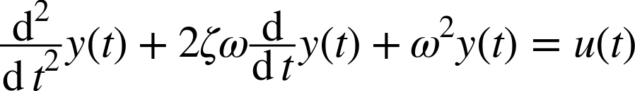
Whereas classical control theory relies on transforms to the frequency domain, state-space methods are based on linear algebra.^[33] The theoretical development begins with the realization that any linear differential equation, regardless of its order, can be written as a linear system of first-order equations by introducing additional variables. As an example, consider the familiar second-order equation that describes a harmonic oscillator:

If we introduce the new variable

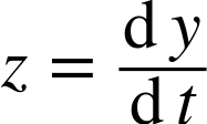
then the original second-order equation can be written as a system of two coupled first-order equations:

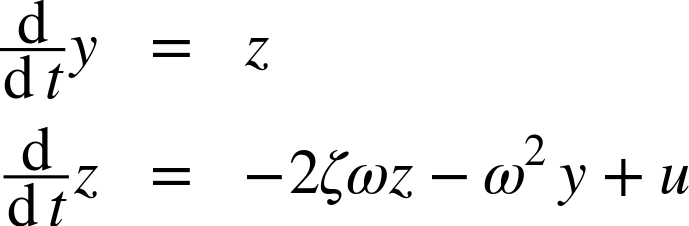
Clearly, the process can be extended to equations of higher order if we introduce more variables. It is easy to treat vector-valued equations or systems of equations this way by turning each component of the original vector into a separate first-order equation.

These equations can be written in matrix form (where a dot over a symbol indicates the time derivative) as follows:

In general, any system of linear, first-order equations can be written in matrix form as

where x and u are vectors and where A and B are matrices. Because there are always as many equations as variables, the matrix A is square; however, depending on the dimension of input u, the matrix B may be rectangular.

Such a system of linear first-order differential equations always has a solution in terms of the matrix exponential:

Here x₀ is a vector specifying the initial conditions, and the matrix exponential is defined via its Taylor expansion:

Now consider the following feedback system:

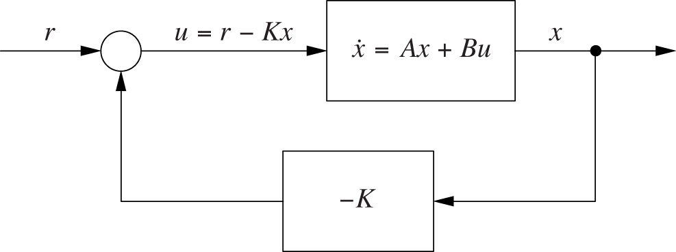
In contrast to what we have seen in the preceding chapters, the information about the system’s dynamic behavior is not provided through its transfer function in the frequency domain. Instead, that information is specified explicitly through the system of differential equations.

The controller K is a matrix, yet to be determined, that acts on (is multiplied by) the system’s output x. Given the setpoint r, we can therefore express the system’s control input u as follows:

Plugging this expression into the differential equation that describes the system yields

This equation is the equivalent of the “feedback equation” (Chapter 21) for the state-space representation.

The matrix (A – BK) determines the dynamics of the closed-loop system; specifically, the eigenvalues ω_j of this matrix correspond to the individual modes of the dynamical system (as discussed in Chapter 23). As mentioned earlier, the solution to the differential equation is given by the matrix exponential. Inserting the matrix (in diagonalized form) into the matrix exponential leads to terms of the form e^ω_jt, so that ultimately the time evolution of the dynamical system is again represented as a linear superposition of harmonic terms.

So in order to design a closed-loop system that has the desired behavior, we must “assign the system’s eigenvalues” to the appropriate values. (This is equivalent to “placing the system’s poles” when working in the frequency domain.) Recall that A and B are determined by the system itself but that the controller K is still completely undetermined. It turns out that under certain conditions it is possible to move the eigenvalues of the closed-loop transfer matrix (A – BK) to arbitrary locations by adjusting the entries of K. Moreover, it is possible to write down explicit expressions that yield the entries of K directly in terms of the desired eigenvalues.

This is a considerable achievement. By following the program just outlined, it is possible to design a closed-loop system having any desired dynamic behavior. Once the desired behavior has been specified (in terms of the eigenvalue positions), the controller can be calculated in a completely deterministic way.

It is instructive to compare this approach with frequency-domain methods. There, the form of the controller was fixed to be of the PID-type; the only means to adapt it to the particular situation was to find the best values for its two (or three) gain parameters. Now, the form of the controller is much less constrained (it is only required to be linear), and its entries are determined completely in terms of the desired behavior. Whereas frequency methods required the “tuning” of a predetermined controller, state-space methods amount to “designing” or “synthesizing” the controller from scratch.

Beyond their immediate application to controller design, state-space methods also allow for new ways to reason about control systems. In particular for systems involving multiple input and output signals, state-space methods enable new insights by bringing methods from linear algebra and matrix analysis to bear on the problem.

For systems involving multiple input and output channels, the question arises under what conditions the inputs are sufficient to establish control over all the outputs simultaneously. It is intuitively plausible that, if a system has fewer inputs than outputs, then in general it won’t be possible to control the values of all the outputs simultaneously. State-space methods help to make this intuition more precise by relating it to questions about the rank of certain matrices that are derived from the matrices A and B determining the controlled system.

To summarize, state-space methods have several advantages over the classical theory:

At the same time, however, state-space methods also have some serious drawbacks:

The last point brings up the issue of robustness, which is the topic of the next section.

The controller-design program outlined in the previous section seemed foolproof: once the desired behavior has been specified in terms of a set of eigenvalue positions, the required controller is completely determined by a set of explicit, algebraic equations. What could possibly go wrong?

Two things, in fact. First of all, it is not clear whether a controller “designed” in this way is feasible from a technical point of view: the control actions required may be larger than what can be built with realistic equipment. But beyond these technical issues, there is a deeper theoretical problem: the controller that was found as solution to the algebraic design problem may be suitable only for precisely that particular problem as expressed in the differential equations describing the dynamical system. In reality, there will always be a certain amount of “model uncertainty.” The physical laws governing the system may not be known exactly or some behavior was not included in the equations used to set up the calculation; in any case, the parameters used to “fit” the model to the actual apparatus are known only to finite precision. State-space methods can lead to controllers that work well for the system as specified yet perform poorly for another system—even if it differs only minimally from the original one.

The methods known as robust control address this issue by providing means to quantify the differences between different systems. They then extend the original controller design program to yield controllers that work well for all systems that are within a certain “distance” of the original system and to provide guarantees concerning the maximum deviation from the desired behavior.

This topic can quickly become quite involved.

In addition to the momentary performance requirement (in terms of minimum rise time, maximum overshoot, and so on), it may be desirable to optimize the overall cost of operating the control system, typically over an extended period of time. We encountered this consideration in several of the case studies in Part III: if there is a fixed cost with each control action, then naturally we will want to reduce the number of distinct control actions. At the same time, there may also be a cost associated with the existence of a persistent tracking error, so that there is a need to balance these two opposing factors. This is the purview of optimal control.

In some ways, optimal control is yet another controller design or tuning method, whereby instead of (or in addition to) the usual performance requirements the system is also expected to extremize an arbitrary performance index or cost function. The performance index is typically a function that is calculated over an extended time period. For instance, we may want to minimize, over a certain time interval, the average tracking error or the number of control actions.

Optimal control leads naturally to the solution of optimization problems, usually in the presence of constraints (such as limits on the magnitude of the control actions, and so forth). These are difficult problems that typically require specialized methods. Finally, it is obviously critical to ensure that the performance index chosen is indeed a good representation of the cost to be minimized and that all relevant constraints are taken into account.

As the last few sections suggest, the mathematical methods used to study feedback and control systems can become rather involved and sophisticated. The classical (frequency-space) theory uses methods from complex function theory to prove the existence of certain limits on the achievable performance of feedback systems. For example, the “Bode integral formula” states that systems cannot exhibit ideal behavior over the entire frequency range: an improvement in behavior for some frequencies will lead to worse behavior at other frequencies.

The endpoint of this line of study is mathematical control theory, which regards control systems as purely mathematical constructs and tries to establish their properties in a mathematically rigorous way. The starting point is usually the dynamical system (or, more generally, , and strict conditions are established under which, for example, all solutions of this system are bounded and thus indicate stability. The direct application of these results to engineering installations is not the primary concern; instead, one tries to understand the properties of a mathematical construct in its own right.