
Chapter 20. The Transfer Function
As Chapter 3 demonstrated, understanding a system’s dynamic behavior is important for building a stable and well-performing feedback loop. In this chapter, we will first describe how to capture information on a system’s dynamic behavior; we then show how to repackage this information in a way that is particularly convenient for our purposes. The tool that we will use is the transfer function.
Differential Equations
The usual way to describe the time evolution of a system is through differential equations. A differential equation is an expression involving the derivative of a quantity, often together with the quantity itself. Here are some examples of differential equations:

Because the derivative is the rate of change of the quantity, differential equations are the natural way to describe how a system changes over time: they describe the system’s dynamics. “Solving” a differential equation means finding a curve y(t) that, for all times t, fulfills the differential equation. Several analytical and numerical methods exist to find the solution to a given differential equation.
Laplace Transforms
Differential equations provide an especially compact way of describing the dynamics of a system: all possible trajectories, for all times t, can be obtained from the differential equation alone.[21] We now repackage this information in a way that makes it easier to manipulate. Rather than considering the quantities of interest as functions of time, we transform them to the frequency domain or frequency space.
To begin with, consider an arbitrary well-behaved function f(t). We can calculate its Laplace transform F(s) as

where s is an arbitrary complex number. Note that f(t) is a function of t whereas F(s) is a function of s. Since t has dimensions of time and since the exponent of the exponential must be dimensionless, it follows that s must have dimension of 1/time; for this reason, we will refer to it as frequency. Functions of t are said to be in the time domain, whereas their Laplace transforms are in the frequency domain.
As it turns out, the quantity F(s) contains exactly the same information as f(t). We can regain the original function by means of an inverse transformation:
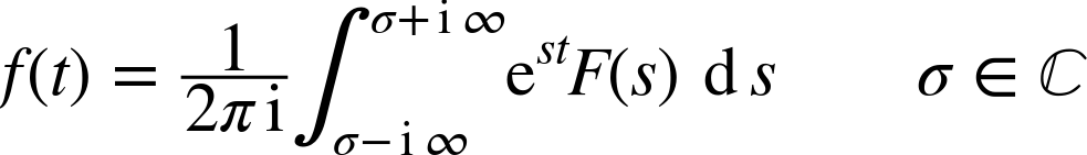
In practice, one rarely finds the Laplace transform of some function (or its inverse) by explicitly evaluating the respective integrals. Transform pairs for most commonly used functions can be looked up in appropriate tables. One can also establish several generally applicable rules to extend the tabulated results to more general cases. (Some transform pairs and rules are shown in Table 20-1. All of these relations are easily verified by performing the transform integral. Every book on control theory will contain such tables, often with many more entries, but Table 20-1 will suffice for our purposes.)

Properties of the Laplace Transform
Given the definition, it is easy to show that the Laplace transform is linear: if h(t) = a f(t) + b g(t), then its Laplace transform is H(s) = a F(s) + b G(s) (where a and b are constant scalars). This property allows us to build up the Laplace transform of a more complicated function (such as a polynomial) from the Laplace transform of its components.
However, the essential property of the Laplace transform—and the real reason we care about it to begin with—is the effect it has on derivatives and integrals.
For example, suppose we want to take the Laplace transform of ![]() , which is the derivative of
f(t). From the definition of the Laplace
transform, we have
, which is the derivative of
f(t). From the definition of the Laplace
transform, we have
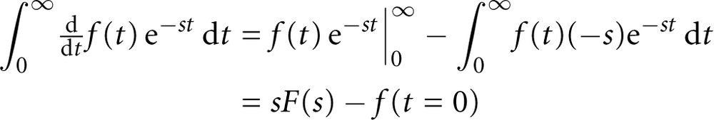
where the integration is performed using integration by parts. In other words, taking the Laplace transform of the derivative of a function amounts to multiplying the transform of the function itself by s. (We pick up an additional term for the value of the function at t = 0. In what follows, we will always assume that the system is initially “at rest,” so that f (t = 0) = 0 and thus we can ignore this term from now on.)
For higher derivatives, we obtain an additional factor of s for each order of the derivative. For integrals, however, we pick up a factor of 1/s—this should not be surprising, since taking the derivative is the inverse operation to performing an integration.
One other operation deserves mention because it occurs frequently in practical applications: if F(s) is the Laplace transform of f(t), then the Laplace transform of f(t – T) is e–sTF(s). In other words, shifting the function in the time domain introduces an exponential factor in the frequency domain. Such shifts are common in control problems, since they describe delays. (If a system replicates its input u(t) to its output y(t) but introduces a delay of duration T, then the output is a shifted version of the input: y(t) = u(t – T).)
We can summarize our discussion as follows:
Taking the derivative in the time domain amounts to a multiplication by s in the frequency domain.
Taking the integral in the time domain amounts to a multiplication by 1/s in the frequency domain.
Shifting the function in the time domain by T to the right introduces a factor e–sT in the frequency domain.
Using the Laplace Transform to Solve Differential Equations
As we have seen, taking the Laplace transform of a derivative replaces each derivative (in the time domain) by a factor of s (in the frequency domain). We can use this property of the Laplace transform to turn differential equations into algebraic equations, provided that the differential equation is linear and has constant coefficients. (A differential equation is linear if the unknown function and its derivatives enter only as linear factors. Of the three differential equations introduced earlier, the first two are linear but the Riccati equation is not—because it contains the term a(y(t))2, which includes the unknown function y(t) raised to the second power.)
A Worked Example
As an example, let’s consider the following simple linear differential equation:

This equation describes various decay processes. If we initially ignore the term u(t), then the change in y(t) is proportional to the current magnitude of y(t). Moreover, as long as the constant T is positive, the change is negative. This means that y decays at a constant rate given by 1/T. A radioactive sample undergoing nuclear decay behaves this way; during each time interval, a specific fraction of the atoms in the sample decay. The differential equation also describes a heated body that is cooling down, because the body loses a fraction of its heat per unit of time.
The term u(t) stands for any type of additional change in y(t) that is independent of the system’s internal dynamics. For instance, u(t) might describe heat that is supplied to the body by an external source. What’s important is that u(t) is independent from the mechanisms that govern the changes in the system itself: it describes an external influence.
It is customary to bring all terms depending directly on the unknown quantity y(t) on the lefthand side, thus:

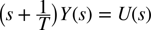
To “solve” this differential equation, we need to find an explicit expression for u(t) that holds for all times t. We will now do so by using the Laplace transform. First, we transform all functions that depend explicitly on time t into functions of frequency s. The differential equation now becomes

Observe that this equation is simply an algebraic equation—all derivatives have been replaced by factors of s. Hence we can now factor out the term Y(s) on the left-hand side:
and solve for Y(s):

We have now “solved” the differential equation, because we have completed our program to obtain an explicit expression for the unknown quantity. Furthermore, this expression is valid for all possible external influences! The problem is that we have only obtained an expression in the frequency domain. To find the behavior in the time domain, we must transform the expression for Y(s) back; this can be done once the shape of the external influence has been fixed.
The Transfer Function
The solution to the differential equation that we found in the previous section had the following structure:
Here the term H(s) does not depend on the external “forcing” function U(s) in any way: it is completely determined by the differential equation alone. In this way, it encapsulates all the internal dynamics of the system. All the information that is contained in the differential equation about the behavior of the system is now contained in H(s). But because H(s) is simply a function of s, H(s) is easier to work with than using the differential equation directly. The function H(s) is known as the transfer function of the system.
Using the Laplace transform, any linear differential equation with constant coefficients can be repackaged into a transfer function. The transfer function can be used to calculate how the system will respond to an arbitrary external influence: just multiply H(s) by the Laplace transform of the influence, and then transform the result back into the time domain. Because the transfer function does not depend on the external forcing function, we can find the response of the system to any external influence in this way.
Moreover, it is often not even necessary to perform the back-transformation to the time domain. Much information about the dynamic behavior of the system can be obtained merely from the structure of the transfer function alone. In particular, the locations where the transfer function becomes infinite or zero (its poles and zeros) let us predict how the system will respond to an external disturbance. This will be the topic of Chapter 23 and Chapter 24.
Worked Example: Step Response
Let’s work out the step response of the system just described. The differential equation ![]() describes its dynamics, and its transfer function H(s) is
describes its dynamics, and its transfer function H(s) is

which has been normalized, so that its steady-state (or zero-frequency, s = 0) gain is unity.
As input to this system we choose a step function u(t) = 1 for t > 0; according to Table 20-1 this function the Laplace transform
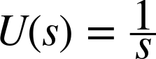
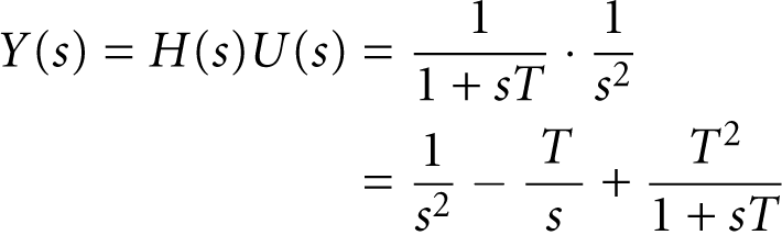
In frequency space, applying an input to a system amounts to multiplying the system’s transfer function by the Laplace transform of the input

In the second step here we have split the expression into partial fractions. (Just add the two terms together to convince yourself that this is indeed correct.)
The quantity Y(s) is the step response in the frequency domain. In order to find the form of the step response in the time domain, we need to transform this expression back. Using Table 20-1 again, we find that
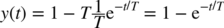
We can now see why this process is commonly known as “simple lag”: the output basically follows the step input but is lagging behind. The response is also simple, without oscillation or other notable behavior.
The simple lag is an extremely important process for practical applications, since it provides the simplest description of any “sluggish” process that basically follows its input. (The process models used in Chapter 8 and Chapter 9 were for the most part based on this type of behavior.)
Worked Example: Ramp Input
In the previous section we found the behavior of a system when subjected to a steplike input. To find the response to a different input, we need only multiply the transfer function by the appropriate input function. For example, if we want to know how the system behaves when we apply a “ramp input” u(t) = t, then we must first find the Laplace transform of the ramp; according to Table 20-1, this is U(s) = 1/s2. We now multiply this input by the transfer function:
This expression can be transformed back into the time domain, term by term. The final result is

This example demonstrates how the transfer function makes it (relatively) easy to find the response to an arbitrary input. Just multiply by the desired forcing function in the frequency domain, and transform back into the time domain.
The Harmonic Oscillator
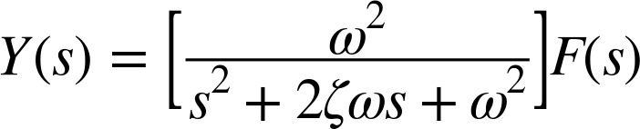
Another example of considerable practical importance is the harmonic, damped oscillator driven by an external force f(t). It has the following differential equation:

If we take the Laplace transform of all functions that depend on t while accounting for the effect the Laplace transform has on derivatives, then the preceding differential equation becomes
Solving for Y(s) yields
and so the transfer function for the harmonic oscillator is
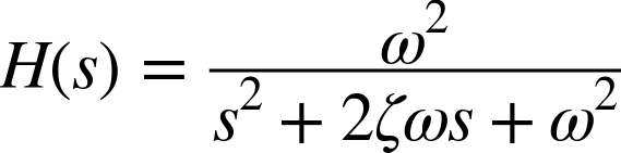
This result is of tremendous practical importance because so many mechanical and electrical systems have a tendency to oscillate. The harmonic oscillator serves as a description of (or at least an approximation to) all such systems.
What If the Differential Equation Is Not Known?
The methods developed in this chapter all assume that the differential equation describing the system dynamics is known explicitly. For many mechanical or electrical systems, this is true because the governing laws are well known. For automation processes, however, this is often not the case. Not only may the actual dynamic behavior be entirely unknown, but it may not even be clear what “laws” might describe it—what would take the equivalent place of Newton’s laws for, say, a web cache?
Despite these objections, the techniques developed in this chapter (and in those that follow) are still relevant for two reasons. First, even if the dynamics of a system are not known a priori, we can still measure its behavior and build a transfer function based on the experimental observations (rather than deriving the transfer function from a differential equation; this was the topic of Chapter 8). Furthermore, the concepts and arguments regarding the dynamic behavior of a system are the same, regardless of whether a differential equation is known explicitly or not.
[21] To pick out one specific trajectory from all possible ones, one also needs to specify its value for t = 0, the initial condition.