
MIMO PLC Electromagnetic Compatibility Statistical Analysis
CONTENTS
7.2.2 General Requirements for the Measurements
7.3.2 Calculation of the Radiation Measure (A:-Factor)
7.4 Statistical Evaluation of ^-Factor Results
7.5 Subjective Evaluation of the Interference to Radio Broadcast
7.5.1 Verification and Calibration
7.6 Interference Threshold of FM Radio Broadcasts
This chapter describes a field measurement campaign performed under the umbrella of ETSI [1] and STF410 [2–5]. The radiated E-field was recorded from power line communication (PLC) signals injected into the mains grid within private homes. Due to the special interest in multiple-input multiple-output (MIMO) PLC, the radiations for all potential feeding possibilities were compared. Furthermore, interference tests were conducted with frequency-modulated (FM) radio receivers.
Electromagnetic interference (EMI) properties of the low-voltage distribution network (LVDN) can be recorded in the time domain (TD) or in the frequency domain (FD). An example of a record in the TD is a continuous transmission of a pseudo-random sequence where the receiver calculates the correlation to derive the channel’s impulse response. An FD measurement is typically done by network analysers (NWAs) when sweeping a carrier over the frequency range of interest. A receiver monitors the channel’s modification of the carrier in amplitude and phase. The pros and cons of each measurement method were evaluated at the beginning of the measurement campaign. It was concluded that the FD approach is better suited for the following reasons:
• Most of the earlier PLC electromagnetic compatibility (EMC) measurements were performed in FD. Thus, a comparison of the results obtained by previous measurements and this campaign is facilitated.
• The human ear is vitally an FD analyser.
• Interferences assessed by human ears like the signal, interference, noise, propagation and overall (SINPO) measurements use consumer electronic devices like amplitude-modulated (AM) or FM radio receivers. Such measurements were performed in ETSI TR 102 616 [6] and ITU-R [7] earlier. Test signals are fed to all transmitter (Tx) paths simultaneously or sequentially. These investigations are conducted with a pulsed signal to allow recognition by the human ear–brain chain.
• Field levels are monitored with a calibrated antenna, which is straightforward to process in FD. EMI measurements in TD have the risk that periodicities in the transmitted PN sequence may cause additional spurs. Furthermore, the measurement dynamics do not seem to be adequate.
• FD measurements can be done using a comb generator and spectrum (or EMI) analyser. This set-up has the benefit that transmitter and receiver do not need to be synchronised. On the other hand, the dynamic range or frequency resolution is limited as feeding energy from the comb generator has to be shared among all signal carriers.
Alternatively, a sweeping source like an NWA might be used. Special care must be taken with signals received by the antenna, as they can be influenced by additional signals being picked up through the long cables connecting the antenna to the NWA. To minimise this effect, double-shielded cables, common-mode absorption devices (CMADs) and ferrites have to be installed (see Chapter 1). This measurement method was selected for faster recoding of frequency sweeps and the high dynamic range.
Measurement campaigns were conducted in Germany, Switzerland, Belgium, France and Spain. To guarantee comparability of the data recorded in each country, all teams were equipped with identical probes or PLC couplers. The antenna was shipped to each team in turn. The actual measurements were performed with a general purpose NWA.
A commercially available, small biconical antenna (with built-in amplifier) was used because of its frequency range of up to 100 MHz. In one location, the loop antenna (limited to frequencies up to 30 MHz) was used in order to have a comparison for the results obtained by earlier measurement campaigns. Figure 7.1 shows the measurement set-up used for the EMI radiation measurements.
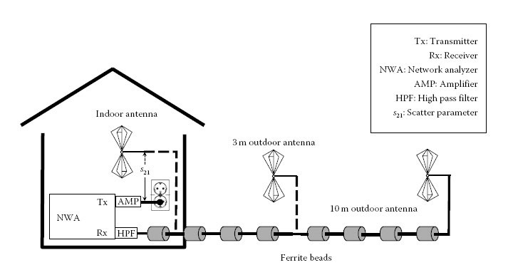
FIGURE 7.1
Measurement set-up arranged in private home.
7.2.2 General Requirements for the Measurements
The test signals for all EMI measurements are fed using MIMO PLC couplers. These couplers as well as the preparation of the power supply for the measurement equipment is described in Chapter 1.
The radiation measurement set-up basically consists of an NWA connected with a MIMO PLC coupler to the mains. To enhance the dynamic range of the set-up, the NWA is connected to an amplifier (AMP) and the amplified signal is fed into the MIMO coupler. The signal has to be at least 10 dB above the noise floor, that is, the signal indicated by the NWA without the signal injection connected. Care should be taken that the output power does not exceed 1 W to avoid damaging the couplers and disturbing the appliances connected to the mains grid. On the other side, the antenna is connected through a cable with ferrites as shown in Figure 7.1 to a high-pass filter (HPF) and the receiving end of the NWA. The HPF attenuates signals below 2 MHz, which were identified in a few cases reducing the dynamic range of the NWA.
In the past, NWA k-factor measurements using coaxial cables to connect the couplers were considered unacceptable, as results may be influenced by signals picked up by the cable. Therefore, the coaxial measurement set-up (including the ferrite beads) described herein was validated by comparative measurements using fibre-optical link equipment between the antenna and the NWA. No difference could be detected. Thus, the fibre-optical link was not further used, because of its reduced dynamic range, higher noise floor and its more cumbersome installation.
The outlets where PLC signals were fed were arbitrarily selected from within the building. The antenna is positioned at a distance of 10 or 3 m from the exterior wall outside the building (see Figure 7.1).
The NWA needs to be calibrated in order to eliminate the effects caused by using long cables in the building. A response (‘through’) calibration is done by shortcutting the endings of both coaxial cables. A conventional adapter (BNC female to BNC female) is used as calibration kit. The MIMO coupler is considered to be part of the PLC channel.
7.3.2 Calculation of the Radiation Measure (k-Factor)
The coupling factor or k-factor is the ratio between the electrical field caused by signal radiation and the signal power fed into the main grid. The k-factor was used first in ETSI TR 102 175 [8].
The radiation of buildings is evaluated by
(7.1) |
where
kEH is k-factor in dB(μV/m)–dBm with regard to the electric component (kE) or in dB(μA/m)–dBm with regard to the magnetic field component (kH)
Eantenna is the electrical field strength in dB(μV/m) received at the location of the antenna
Pmax,feed is the signal power in dBm at the output of the PLC coupler (in case of terminated output)
UReceiver is the voltage in dB(μV) at the output of the antenna
AF is antenna factor in dB(1/m) of the antenna
Pmax,amp_output is signal power in dBm at the output of the amplifier (in case of termination)
APLC_Coupler is the attenuation of the PLC coupler in dB ETSI TR 101 562-2 [4]
PReceiver is the power from in dBm the output of the antenna
ConvdBm2dBμV is the conversion factor from dBm to dBμV in a 50 Ω environment: 107 dBμV–dBm (see Chapter 6)
s21 is the scattering parameter in dB as measured by the calibrated network analyser (as shown in Figure 7.1)
The literal meaning of the formula earlier is as follows: If a signal is fed with 0 dBm into the mains of a building, then an electrical field of Eantenna dBμV/m is recorded inside as well as outside the building.
From the recorded values s21 of the NWA, the k-factor can be derived using Equation 7.1.
The combinations of different antenna polarisations or orientations are antenna dependent. The calculations presented in Table 7.1 apply to derive a single k-factor for each injection, plug and antenna location combination. Loop antennas capture signals only from one orientation or direction. The circumpolar symmetry of the biconical consequences signals to be picked up from two directions. The first orientation is the one where the antenna spots to where the second one is the horizontal or vertical orientation (as set up by the operator). The resulting field is derived after calculating the maximum of the two biconical records or the vector sum of the three dimensions individually measured using the loop antenna.
Calculation of Resulting k-Factor in Dependence of Antenna Type
Antenna Type |
Calculation of the Resulting k-Factor |
Biconical |
kres = max(khorizontal, kvertical) |
Loop |
where x, y and z are the three orientations |
These calculations are performed individually for each frequency in each record.
7.4 Statistical Evaluation of k-Factor Results
The k-factor was measured at 15 locations in Spain, France and Germany.
A typical sweep from 1 to 100 MHz of any k-factor measurement is shown in Figure 7.2. Fading characterises the shape of a k-factor sweep. The legend of Figure 7.2 says that the signals are fed to outlet No. ‘01’ for this record. The feeding port was ‘LNNT’, which is the D1 of the MIMO PLC coupler displayed in Chapter 1. The abbreviation represents ‘live to neutral’; other ports are ‘not terminated’, which is the single-input single-output (SISO) feeding case; and ‘A03_D0’ is the antenna position number 3 at a distance of 10 m from the outside wall of the building (symbolised by ‘D0’).
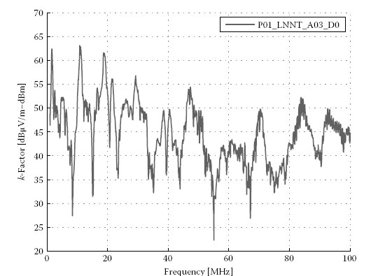
FIGURE 7.2
Typical sweep of a k-factor measurement outdoors at 10 m distance.
In total, 1294 such sweeps were recorded in this measurement campaign.
Figures 7.3 and 7.4 show the median of all data separated into the individual feeding possibilities. The median value for each measured frequency and feeding style is calculated individually. The values here are derived from data received from all antenna locations indoors and outdoors at 3 and 10 m distance from the building. For MIMO PLC, a comparison to the traditional SISO feeding style is interesting. All median values in Figures 7.3 and 7.4 are shown relative to SISO.
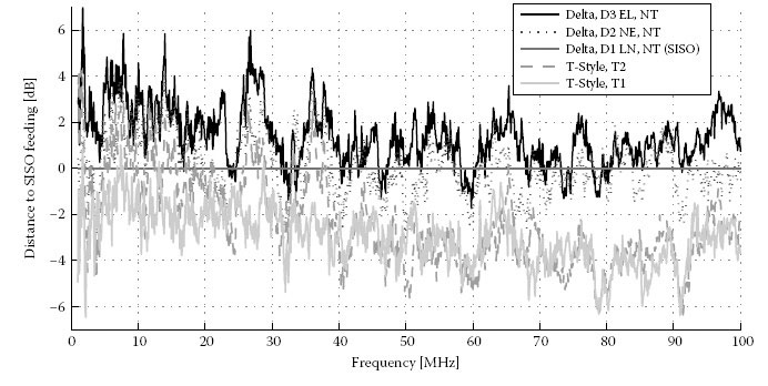
FIGURE 7.3
Median values for non-terminated delta- and T-style feeding possibilities. Outlet or antenna position always matches at comparisons relative to SISO.
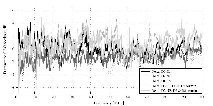
FIGURE 7.4
Median values for delta feeding possibilities Outlet or antenna position always matches at comparisons relative to SISO.
Figure 7.3 presents the unterminated delta- and T-style feeding. The SISO case (from live neutral [LN] and not terminated [NT]) is one of them. It is the straight 0 dB line. Figure 7.4 depicts the terminated delta feedings. Either all delta ports are terminated or only 2 out of the 3 are terminated, as indicated in the legend. The three-port termination (D1, D2, D3) feeds 1.3 dB less energy into the mains after the PLC coupler compared to one-port termination (D1 NT, D2 NT, D3 NT on the left side). The feeding style causing the highest E-fields is the unterminated D3. The reason could be the absence of any devices connected to the mains between protective earth and live. There are no resistors present consuming the HF power between these ports. The two T-style couplings show the lowest potential for interference. This is valid for the full monitored frequency range. Apparently, they meet the best symmetry in the mains grid.
The median k-factor value of each location is given in Table 7.2 for all antenna positions indoors and at 3 and 10 m distance from the outside wall of the building.
Due to the high variance of the results between the individual locations and the low number of locations surveyed, a statistical evaluation of the k-factor for each country has not been calculated Furthermore, the number of records from each location is unique and given in Table 7.2 in brackets. The number of antenna positions was selected according to the size of the location, size of the garden and accessibility to each location. In total, in all frequencies and feeding possibilities, 771,682 values (482 sweeps) have been recorded from a 10 m distance, 650,006 values (406 sweeps) from 3 m and 441,876 values (276 sweeps) from indoors. An explanation why there is such a high spread in the median values might be due to local conditions surrounding the building and inside the flat. In most measurements conducted, the area around the building was flat and the outdoor antenna positions were located on the same level as the ground floor. If the residential unit was a flat located on the second floor of a building or a multi-level house, then some of the feeding outlets had an additional vertical distance to the antenna. For example, the k-factor measurements in France and the location Voerde in Germany were recorded where all feeding outlets were located on the ground floor and the area around the building is flat land. This is why the outdoor k-factors at these locations tend to be higher than at others.
Median Coupling Factors of Each Location
Location |
Country |
Median k-Factor Indoor in dBμV/m–dBm (No. of Records) |
Median k-Factor from 3 m Distance in dBμV/m–dBm (No. of Records) |
Median k-Factor from 10 m Distance in dBμV/m–dBm (No. of Records) |
Duerrbachstr |
Germany |
72.60 (38,425) |
Not measured |
45.63 (76,849) |
ImGeiger |
Germany |
69.17 (51,233) |
Not measured |
44.77 (102,465) |
Nauheimerstr |
Germany |
73.48 (51,233) |
Not measured |
43.24 (102,465) |
Rothaldenweg |
Germany |
73.60 (12,809) |
Not measured |
51.54 (102,465) |
Schlossbergstr |
Germany |
68.46 (38,425) |
57.10 (115,273) |
44.74 (76,849) |
VickiBaumWeg |
Germany |
61.19 (51,233) |
Not measured |
47.70 (102,465) |
Boenen |
Germany |
71.88 (38,425) |
62.38 (25,617) |
Not measured |
Universitaet |
Germany |
Not measured |
55.58 (12,809) |
49.84 (12,809) |
Voerde |
Germany |
Not measured |
69.53 (60,839) |
59.76 (60,839) |
El_Puig |
Spain |
55.89 (48,031) |
40.04 (144,091) |
Not measured |
Sant_Sperit |
Spain |
Not measured |
49.51 (144,091) |
44.87 (48,031) |
Torre_en_Conill |
Spain |
57.83 (48,031) |
45.12 (96,061) |
31.87 (48,031) |
Guingamp |
France |
72.92 (25,617) |
59.52 (25,617) |
54.22 (12,809) |
RueBunuel |
France |
69.61 (12,809) |
Not measured |
52.67 (12,809) |
RueDepasse |
France |
70.67 (25,617) |
62.89 (25,617) |
50.69 (12,809) |
All locations |
67.98 |
51.3 |
46.96 |
The complementary cumulative distribution (C-CDF) of the k-factor at a location where all three antenna positions were recorded is depicted in Figure 7.5.
The k-factor records presented earlier were obtained using an E-field antenna, because magnetic EMC antennas are not available for frequency ranges up to 100 MHz. Furthermore, consumer electronic devices in private homes use an E-field antenna (stick or whip) in the HF and VHF bands. The marker in Figure 7.5 is to be interpreted as ‘in 20% of all records in a 3 m distance from the house, the k-factor was larger than 51.6 dBμV/m–dBm’.
Comparisons between the magnetic field (H-field) and electric field (E-field) were recorded at the location in Voerde, Germany. Radiation measurements were recorded from the building using an E-field biconical antenna [9] and H-field ring antenna [10], from 3 and 10 m away, with the antennas in the same fixed position for each reading. In order to compare H- and E-field values, the magnetic fields – recorded in dBμA/m – need to be converted into electric fields with a free space wave impedance of 377 Ω = 51.5 dBΩ. Figure 7.6 shows low correlation between H- and E-fields at 3 m distance. Obviously, a distance of 3 m may still be in the near field, where the free space wave impedance of 377 Ω cannot be applied. At 10 m from the building, the E- and H-fields display a similar pattern, as expected in the far field (see Figure 7.7), especially for frequencies higher than 15 MHz. The graphs stop at 30 MHz because the loop antenna [10] is only specified up to this frequency. At frequencies above 30 MHz, it is expected that far-field radiation conditions from a building are valid at closer distances or even indoors.
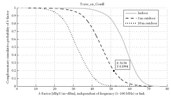
FIGURE 7.5
C-CDF of k-factor of a location. Note: Number of sweeps indoor, 33; in 3 m, 66; and in 10 m, 33.
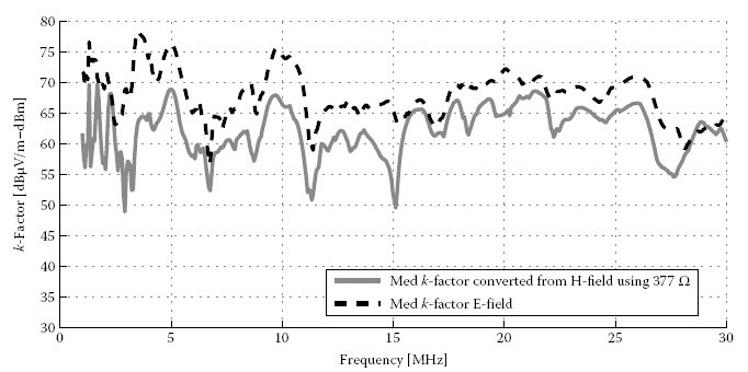
FIGURE 7.6
k-Factor measured with biconical and loop antenna at 3 m distance at one location.
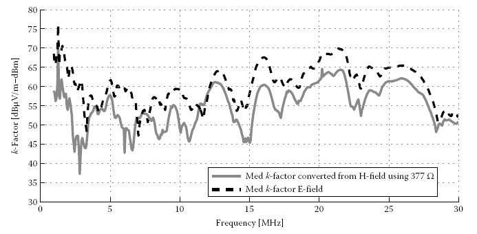
FIGURE 7.7
k-Factor measured with biconical and loop antenna at 10 m distance.
7.5 Subjective Evaluation of the Interference to Radio Broadcast
Subjective evaluations of interference to AM radio reception in the high-frequency (HF) bands were performed in the past in TD ETSI TR 102 616 [6]. Performing identical tests with all MIMO feeding possibilities would deliver unstable results, because the variance of received signal level (fading in TD) is more dynamic than an operator might be able to test. During a MIMO test, the interference from all MIMO feeding possibilities should be compared. The signal level is usually never stable in HF bands. Schwager [11] describes dynamic changes in the received HF signal level caused by reflections on the ionosphere. Broadcasting conditions in the very high-frequency (VHF) band are by far more stable over time, allowing a comparison of levels recorded over a period of a few minutes.
The source of the signal is a broadband noise generator and a frequency modulator shifting the noise to the desired frequency. The generator can be switched on and off, in order to distinguish the disturbed and undisturbed states. The FM-modulated signal is injected as an interfering signal to the mains using all possible feeding styles of the MIMO coupler shown in Chapter 1.
7.5.1 Verification and Calibration
Prior to the test, the disturbance signal has to be analysed with a measurement receiver or spectrum analyser to document the 3 dB bandwidth. As a first step, the amplification between the generator output level and the signal injected into the Bayonet BNC plug of the MIMO PLC coupler has to be determined. The feeding level of the signal generator is Umax_feed.
At each frequency of a selected radio station, the level of the RF generator is adjusted to a lower level where no disturbance at the radio receiver is recognised. From that value, the generator level is increased until a disturbance can hardly be recognised. After that the level of interference signal, Ugen in dBμV is verified and documented.
This procedure is repeated for each
• Coupling type
• Selected frequency
• Feeding outlet (injection point)
• Radio receiver
• Radio receiver location
Furthermore, the measurements have to be done when the radio receiver is battery driven and mains powered.
7.6 Interference Threshold of FM Radio Broadcasts
The level of interference in FM radio broadcasts was tested at 10 different locations. The field test set-up is shown in Figure 7.8. In total, 1179 subjective evaluations of PLC interference, which can be detected by human ears, in FM radio were conducted. This includes nine feeding styles times 131 radio stations with various radio devices in a range of different positions. The threshold at which human ears are able to detect interference is noted in the measurement protocol.
Figure 7.9 shows the C-CDF of the threshold of all radio services at all locations independent of the radio device or power supply used. The x-axis is the feeding PSD injected to a power outlet. All MIMO feeding styles are within the black area, and the three delta feedings are explicitly given. The FM services received with a low signal level are interfered also with low PLC feeding levels. As shown in the top left corner of Figure 7.9, there is only a small variation between the individual feeding styles. Sensitive FM stations do not show higher or reduced interference potential when another feeding style is selected.
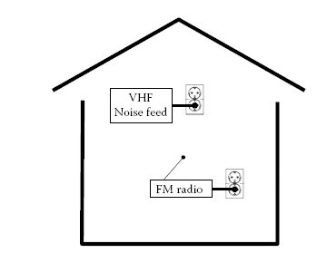
FIGURE 7.8
Basic set-up for FM interference tests.
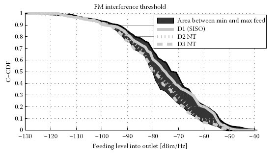
FIGURE 7.9
C-CDF of threshold when interference is noticeable by human ears.
When performing similar tests in the HF range with AM radio stations, a significant difference was found if the radio was battery driven or mains powered [9]. HF radio devices also used the mains grid for communications (like PLC modems). They use the mains as a counterpoise to the whip antenna resulting in a bipolar reception instead of only a monopole. This phenomenon could not be verified in the VHF; the conducted coupling path was not dominant.
Or in other words, the FM radio receivers used in this test are sufficiently isolated from the mains interferer. There was never any influence whether the FM radio was mains powered or battery driven.
The FM radio immunity field tests were performed using radio receivers operated by the habitants of the flats. The immunity of all radio devices was pretty much identical. No dependency among device manufacturers or HIFI radio systems versus kitchen radios could be found.
EMI field tests were conducted measuring the PLC’s radiation from buildings as well as the interference to FM radio receivers. The results show all three wires connected to power outlets in private homes to have a similar potential for interference. No significant difference was found when injecting signals into the mains in any MIMO feeding style compared to the traditional SISO style. Chapter 16 shows further experiments of the influence of beamforming on the radiated fields.
1. European Telecommunications Standards Institute, http://www.etsi.org, accessed April 2013.
2. Special Task Force 410. http://portal.etsi.org/STFs%5CToR%5CToR410v11_PLT_MIMO_measurem.doc Members to STF410: Andreas Schwager (STF Leader), Sony, Germany; Werner Bäschlin, JobAssist, Switzerland; Holger Hirsch, University of Duisburg-Essen, Germany; Pascal Pagani, France Telecom, France; Nico Weling, Devolo, Germany; Jose Luis Gonzalez Moreno, Marvell, Spain; Hervé Milleret, Spidcom, France. STF410 produced following technical reports: [ETSI TR 101 562-1]; [ETSI TR 101 562-2]; [ETSI TR 101 562-3].
3. ETSI TR 101 562-1 V1.3.1 (2012-02), PowerLine Telecommunications (PLT); MIMO PLT; Part 1: Measurement methods of MIMO PLT.
4. ETSI TR 101 562-2 V1.3.1 (2012-10), PowerLine Telecommunications (PLT); MIMO PLT; Part 2: Setup and statistical results of MIMO PLT EMI measurements.
5. ETSI TR 101 562-3 V1.1.1 (2012-02), PowerLine Telecommunications (PLT); MIMO PLT; Part 3: Setup and statistical results of MIMO PLT channel and noise measurements.
6. ETSI TR 102 616 V1.1.1 (2008-03): PowerLine Telecommunications (PLT); Report from Plugtests™ 2007 on coexistence between PLT and short wave radio broadcast; Test cases and results.
7. ITU-R Recommendation BS. 1284: General methods for the subjective assessment of sound quality.
8. ETSI TR 102 175 V1.1.1 (2003-03): PowerLine Telecommunications (PLT); Channel characterization and measurement methods.
9. SCHWARZBECK MESS – ELEKTRONIK; EFS 9218: Active electric field probe with biconical elements and built-in amplifier 9 kHz … 300 MHz.
10. R&S®HFH2-Z2: Loop Antenna Broadband active loop antenna for measuring the magnetic field-strength; 9 kHz–30 MHz.
11. A. Schwager, Powerline communications: Significant technologies to become ready for integration, PhD dissertation, Universität Duisburg-Essen, 2010, http://duepublico.uni-duisburgessen.de/servlets/DerivateServlet/Derivate-24381/Schwager_Andreas_Diss.pdf.