1. Introduction to Power Line Communication Channel and Noise Characterisation

Since the late 1990s, an increased effort has been put into the characterisation of power line communication (PLC) channels with the aim of designing communication systems that use the electrical power distribution grid as data transmission medium.

Reliable PLC systems, for home networking, Internet protocol television (IPTV), Smart Grid and smart building applications are now a reality. However, power lines have not been designed for communication purposes and constitute a difficult environment to convey information via early analogue signalling or nowadays widespread advanced digital PLC systems. The PLC channel exhibits frequency-selective multi-path fading, a low-pass behaviour, cyclic short-term variations and abrupt long-term variations that are introduced in Section 1.5. Further, power line noise can be grouped based on temporal as well as spectral characteristics. Following, for example [5,6], one can distinguish coloured background noise, narrowband (NB) noise, periodic impulsive noise (asynchronous or synchronous to the alternating current [AC] frequency), as well as aperiodic impulsive noise (see Section 1.6). These impairments are leading some researchers to speak of a ‘horrible channel’ [7].

Apart from these, the very principle of PLC implies that small-signal, high-frequency technologies are being deployed over power-carrying cables and networks that were designed for electricity transmission at low frequencies. In terms of voltage, the equipments’ communication ports would fail if they were connected directly to the power grid. This is similarly true when looking at PLC testing and measurement equipment, such as a spectrum analyser, which is why PLC couplers are needed to couple the communication signal into and out of the power line while at the same time protecting the communication equipment. Couplers may be of either inductive or capacitive nature with detailed coupling schemes introduced in Section 1.3. Before that, however, this chapter looks at PLC frequency bands and common topologies in Section 1.2 as these are possibly the most profound stage setters when characterising PLC channel and noise scenarios. In the sequel, the aim of Section 1.4 is to provide information on measurement equipment and procedures that have been used to generate a plurality of results for various chapters throughout this book. Further, Sections 1.5 and 1.6 introduce the underlying concepts of PLC channel and noise modelling, respectively, and guide the reader to the more detailed chapters on each topic. This chapter is rounded off by an appendix that explains the basics of dual conductor transmission line theory, considered interesting background reading for those new to PLC signal propagation.

1.2 PLC Frequency Bands and Topologies

The frequency bands – as agreed upon by the International Telecommunications Union [8] – are shown in Figure 1.1. The band name abbreviations stand for super low, ultra low, very low, low, medium, high, ultra high, very high, super high, extremely high and tremendously high frequency, respectively. As indicated in Figure 1.1, currently only the VLF up to the UHF bands are interesting for PLC systems. These systems are usually subdivided into narrowband (NB) and broadband (BB) PLC; the former operating below 1.8 MHz, the latter operating above [9]. Details on the regulations corresponding to these frequency bands can be found in Chapter 6. An overview on systems that belong to either the class of NB-PLC or the class of BB-PLC can be found in Chapter 10.

Besides the distinction into NB-PLC and BB-PLC, it has been common practice to distinguish power line topologies according to operation voltages of the power lines [2,9,10].

FIGURE 1.1
ITU frequency bands and their usage in power line communications.

High-voltage (HV) lines, with voltages in the range from 110 to 380 kV, are used for nationwide or even international power transfer and consist of long overhead lines with little or no branches. This makes them acceptable wave guides with less attenuation per line length as for their medium-voltage (MV) and low-voltage (LV) counterparts. However, their potential for BB communication services has up to the present day been limited. Time-varying HV arcing and corona noise with noise power fluctuations in the order of several tens of dBs as well as the practicalities and costs of coupling communication signals in and out of these lines have been an issue. Further, there is a fierce competition of fibre optical links. In some cases, these links might even be spliced together with the ground conductor of the HV system [11,12]. Nevertheless, several successful trials using HV lines have been reported in [13, 14, 15, 16].

MV lines, with voltages in the range from 10 to 30 kV, are connected to the HV lines via primary transformer substations. The MV lines are used for power distribution between cities, towns and larger industrial customers. They can be realised as overhead or underground lines. Further, they exhibit a low level of branches and directly connect to intelligent electronic devices (IED) such as reclosers, sectionalisers, capacitor banks and phasor measurement units. IED monitoring and control requires only relatively low data rates and NB-PLC can provide economically competitive communication solutions for these tasks. MV-related studies and trials can be found in [17, 18, 19, 20].

LV lines, with voltages in the range from 110 to 400 V, are connected to the MV lines via secondary transformer substations. A communication signal on an MV line can pass through the secondary transformer onto the LV line, however, with a heavy attenuation in the order of 55–75 dB [21]. Hence, a special coupling device (inductive, capacitive) or a PLC repeater is frequently required if one wants to establish a high data rate communications path. The LV lines lead directly or over street cabinets to the end customers’ premises. Note that considerable regional topology difference exits. For example, in the United States, a smaller secondary transformer on a utility pole might service a single house or a small number of houses. In Europe, however, it is more common that up to 100 households get served from a single secondary transformer substation. Further, as pointed out in [22], significant differences exist between building types. They may be categorised as multi-flat buildings with riser, multi-flat buildings with common meter room, single family houses and high-rise buildings. Their different electrical wiring topologies influence signal attenuation as well as interference between neighbouring PLC networks [23]. In most cases, the electrical grid enters the customer’s premises over a house access point (HAP) followed by an electricity meter (M) and a distribution board (fuse box). From there, the LV lines run in a tree or star topology up to the different power sockets in every room. One frequently refers to PLC systems operating from outside to inside a customer’s premises as access systems while systems operating within the premises are referred to as in-home. It can be summarised that the access scenario establishes data connections to a group of customers through the overhead and/or underground electrical power distribution grid [7,24, 25, 26]. The in-home scenario enables the communication of different devices within a user’s premises [7,27, 28, 29, 30, 31, 32].

Besides these operation voltage-oriented distinctions, one may distinguish in-vehicle PLC and MIMO PLC.

In-vehicle PLC has been considered to provide data access to moving vehicles like trains [33], as well as within the vehicles themselves, for example, in cars [34], aerospace and outer space applications [35,36], ships [37] and submarines [38]. Among others, advantages of PLC over other wireline communication techniques are weight reduction, reduced pin numbers for device internal connections and, in general, wiring complexity reductions. Especially, communicating with parked plug-in electrical vehicles has been at the focus of attention with respect to integrating electrical vehicle fleets into the Smart Grid that is currently built up all around the world [39]. Besides, in-cars PLC is starting to revitalise the after-sales market business for consumer electronics.

MIMO PLC – Building on the success of multiple-input multiple-output (MIMO) signal processing within wireless communications [40,41], it is worth noting that MV and HV installations often make use of four or more conductors. In this respect, a theoretical framework of multi-conductor transmission line (MTL) theory is extensively treated in [42]. Further, in many in-home installations three wires, namely live (L) (also called phase), neutral (N) and protective earth (PE), are common. Exactly how common on a worldwide scale was investigated by the European Telecommunications Standards Institute (ETSI).^* The investigation of Specialist Task Force (STF) 410 [43] was based on

• A study of individual grounding systems and investigations into which grounding systems are used in which countries; such information could be derived from, for example, education material for electricians.

• The creation of a list of AC wall socket types and their respective usage area. For example, universal travel adapters indicate how many different power outlets exist in the world. Plugs and sockets could easily be checked for the presence of a PE pin. However, the existence of the pin does not guarantee the existence of a PE wire leading up to the socket. When renewing older buildings frequently, the protective earth of the socket is shortcut with the neutral wire behind the outlet or simply not connected at all.

• Research on the dates when the PE installation became mandatory in a country and an estimate of how many electrical installations have taken place since then.

• A survey of sales information, for example, worldwide sales numbers of residual-current devices (RCDs) or power cables including ground which in the sequel allows estimates on the PE availability level in a country.

• A worldwide survey of data from electrical standardisation committees and engineering clubs for each country.

Reference [43] lists detailed information and statistical evaluations on each of these points. It is almost impossible to summarise all this information into a single sentence, but when trying to do so, the result would be something like

The third wire is present at all outlets in China and the Commonwealth of Nations, at most outlets in the western countries and only at very few outlets in JP and Russia.

1.3 Coupling Methods

When turning to coupling methods, one may generally distinguish between inductive and capacitive couplers. It should be noted that inductive couplers guarantee a balance between the lines whereas capacitive couplers often introduce asymmetries due to component manufacturing tolerances. Besides symmetry, signal bandwidth and the dimensioning to protect the communications equipment, for example, against lightning strikes or other HV spikes on the grid side are decisive coupler properties. Moreover, the observed channel characteristics are not independent from the coupling devices used to inject and receive the power line signal. Inductive as well as capacitive couplers especially tailored to MV, HV and even up to extra HV lines can be found in ([44, Section 5.5.1]). Further, details on LV inductive single-input single-output (SISO) couplers may, for example, be found in [45,46]. The following will focus on LV inductive MIMO coupling options that play an important role throughout various chapters of this book.

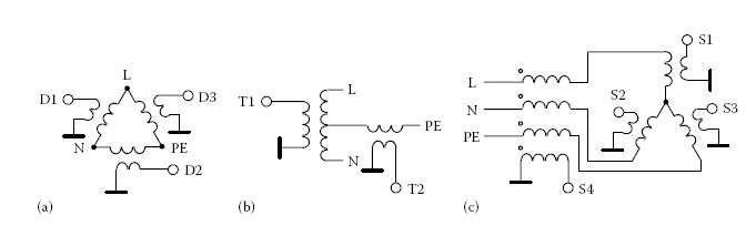
FIGURE 1.2
Inductive MIMO PLC couplers, (a) Delta-style (D), (b) T-style (T) and (c) star-style (S).

Figure 1.2 presents three inductive MIMO coupler options, that is, a delta-style (D) coupler [47], a T-style (T) coupler [48] and a star-style (S) coupler [47]. Coupler designs are tightly related to radiated emission treated in more detail in Chapters 6 and 7. According to the Biot–Savart law, the main source of radiated emission is the common-mode (CM) current denoted I_CM. To avoid radiated emission, traditionally PLC modem manufacturers aim at injecting the signal as symmetrically as possible. This way, 180° out of phase electric fields are generated that neutralise each other resulting in little radiated emission. This desired symmetrical way of propagation is also known as differential-mode (DM) with its associated signal voltage U_DM. In a symmetrical network, the differential current I_DM flows from its feeding point via the network back to its source as indicated in Figure 1.3. In case of asymmetries, for example, caused by parasitic capacitances (inside the refrigerator in Figure 1.3), a small part of the differentially injected radio frequency (RF) current I_DM turns into CM current I_CM. It flows to ground or to any other consumer device and returns to its source via a series of asymmetries in the network. Normally, there are many asymmetries inside a PLC topology. For example, an open light switch causes an asymmetric circuit and, hence, even if only DM is injected by a PLC coupler, DM to CM conversion occurs [49].

Specifically, to avoid additional CM currents, feeding MIMO PLC signals can be done using the delta or T-style couplers from Figure 1.2 while it is not recommended using the star-style coupler – known also as longitudinal coupler – due to the risk of CM signal injection. As shown in Figure 1.2, the delta-style coupler, also called transversal probe, consists of three baluns arranged in a triangle between L, N and PE. The sum of the three voltages injected has to be zero (following Kirchhoff’s law). Hence, only two of the three signals are independent. Turning to the T-style coupler, it feeds a DM signal between L and N plus a second signal between the middle point of L-N to PE. Further details on the pros and cons of each coupler type are discussed in [43].

All three coupler types are well suited for reception. However, especially the starstyle coupler, where three wires are connected in a star topology to the centre point, is interesting. Kirchhoff’s law forces the sum of all currents arriving at the centre point to be zero. Thus, only two of the three receive (Rx) signals are independent. Nevertheless, due to parasitic components the signals at the third port may additionally improve the capacity of MIMO PLC system (see Chapter 5 for details). However, a more significant benefit is the possibility to receive CM signals, that is, a fourth reception path. The CM transformer is magnetically coupled (Faraday type). On average, CM signals are less attenuated than DM signals which makes their reception interesting, especially for highly attenuated channels [47] (see also Chapter 5).

FIGURE 1.3
Generation of CM signals in a building.

In general, looking at the experienced input impedance of a mains network, there might be an impedance unbalanced between L-N and L-PE. This is especially true for lower frequencies where 50 Hz loads play an important role [27]. Further, the effective CM impedance is also very different from DM impedances (see Chapter 5 for details).Table 1.1 shows a summary of approximate expected power line input impedances as obtained from the open literature and other chapters in this book. Table 1.1 shows that, for example, impedances in Europe and the United States are very similar. Comparing L-N with L-PE impedances, a marked difference can be observed. For example, for frequencies below 500 kHz this difference can be more than three times and for frequencies between 1 and 30 MHz the L-PE impedance may be around two times larger than in the L-N impedance. However, when looking at the average statistics up to 100 MHz, impedance levels converge, yielding a more balanced MIMO system, the reason possibly also being that MIMO couplers used in the related measurement campaign terminated all three ports at signal injection. More details are found in Chapter 5.

TABLE 1.1

Power Line Impedances

Frequencies	Country	L-N in Ω	L-PE in Ω	N-PE in Ω	Source
50–500 kHz	JP	0.5–20 (6.5)	na	na	[50,51]
	Germany	1–60 (10)	na	na	Chapter 2
	Europe	na	1–200 (30)	na	[52]
	China	1–9 (5)	na	na	Chapter 3
	United States	na	1–150 (18)	na	[52,53]
1–30 MHz	JP	3–1 k (83)	na	na	[54]
	Germany	10–300 (30)	20–400 (60)	na	[27]
	Europe	(102)	9–400 (90)	na	[47,52]
	United States	na	6–400 (95)	na	[52,53]
1–100 MHz	Europe	10–190 (86)	10–190 (89)	10–190 (87)	Chapter 5

Note: Value in brackets indicates median. If there is more than one reference, the range was taken over the minima/maxima from the references and the arithmetic mean was calculated to obtain a single median value.

Statistical knowledge of the input impedances may be taken into account in the MIMO coupler design. That is, isolation transformers/baluns are required for most MIMO coupling strategies to allow the multiple signals to float independently. In this respect, to obtain BB channel and noise characterisation and EMC results in Chapters 5 and 7, a single coupling circuit – capable of implementing the T-style, delta-style and star-style coupler – as introduced in Figure 1.2, has been designed with its schematic shown in Figure 1.4.

The physical connection to the power grid via a Schuko-type plug is shown on the left. Selection between the coupling types is performed via the switches labelled Sw1 and Sw2, shown in the centre. On the right-hand side, there are the terminals T1 to T2, D1 to D3 and S1 to S4 for connecting the coupler to measurement equipment such as a network analyser (NWA) or a digital sampling oscilloscope (DSO). The delta-style and T-style terminals are connected through current baluns to facilitate floating signals, and further minimise CM injection as well as any subsequent increase in radiation. The baluns in the delta-style coupler are 1:4 Guanella transformers with very low loss. They perform a 50–200 Ω impedance conversion. Considering a DM impedance of any pair of the three wires of 102 Ω where in the MIMO case this impedance exists twice in series plus once in parallel (resulting in 68 Ω), the 200 Ω output of the Guanella transformer appears to be the optimal matching compromise. Sw3 allows toggling between MIMO and SISO terminations of the feeding ports. The star-style terminals use coupled current transformers (CM chokes). Their function is to measure the CM current flowing through the three wires ( $L | | P E | | N$ $L | | P E | | N$ ). The inductance of each winding is selected small enough not to filter the PLC frequencies of interest (1–100 MHz). An additional switch (not shown in Figure 1.4) might short circuit the secondary (and thus magnetising inductance) of these CM chokes, thus making them transparent to the overall circuit when not in use.

Looking at the other electronic components in Figure 1.4, one can see that in series with each line, there is a 4.7 nF coupling capacitor, fulfilling the main coupling function – protection by means of filtering, while the capacitor to the Earth wire is implemented to maintain symmetry. Furthermore, it lowers the leakage current that could otherwise cause a residual current device (RCD) to fail. The breakdown voltage of these capacitors are rated roughly twice the expected root mean square (rms) value, that is, 1.5 times the expected peak value of the power waveform to be blocked. The mains connection can be unplugged at any time. Hence, the capacitors may be charged to dangerous voltages, and they are in this case discharged by a parallel resistor, large enough not to short circuit significant current past the blocking capacitor – thereby impacting on the filtering action of this capacitor. The RC time constant is adjusted so that the blocking capacitor discharge within 15 ms to protect against accidentally touching the prongs of the attached Schuko when unplugging it. Apart from the protection offered by the coupling capacitor, supplementary protective devices are deployed to absorb voltage transients. Surge protection diodes can be seen in parallel with the three lines. The input impedance of these and other protective devices are sufficiently high not to drain or filter the PLC signal. On the mains side of the coupling capacitors (across L-N), gas-discharge devices and metal-oxide varistors (MOVs) are used. They serve as over-voltage protection and are deployed in parallel as they possess different speed versus power characteristics and are, hence, complementary. Supplementary information on surge protection in general may be found in [55, 56, 57, 58]. The specific safety components of the coupler as shown in Figure 1.4 are given in [45] alongside the coupler’s calibration data.

FIGURE 1.4
A 2-Tx 4-Rx MIMO PLC coupler with added protective circuitry. (Based on European Telecommunication Standards Institute (ETSI), Powerline Telecommunications (PLT); MIMO PLT Universal Coupler, Operating Instructions – Description, May 2011. Available online at: http://www.etsi.org/deliver/etsi_tr/101500_101599/101562/01.01.01_60/tr_101562v010101p.pdf.)

1.4 Channel and Noise Measurement Set-Up

This section describes the measurement set-up and the equipment used to record channel, reflection and noise properties of the MIMO PLC channel on a LV grid. It therewith forms the basis for the results in Chapters 5, 7 through 9, 16, 17 and 22. The following measurement campaign objectives are defined:

• Frequency range from 1 to 100 MHz.

• Channel transfer function (CTF) measurements.

• Noise-level measurements.

• Input impedance measurements.

• Coupling factor measurements (i.e.the coupling factor or k-factor is the ratio between the electric field caused by signal radiation and the signal power fed into the main grid [59] [see also Chapter 7]).

• All measurements are to be performed with the same coupler design to allow for straightforward comparability of results.

1.4.1 Transfer Function Measurements

The CTF can be measured in the frequency domain by recording the scattering parameter S₂₁ using a conventional NWA (for an introduction to scattering parameters see, for example, [60]).Figure 1.5 depicts the set-up for channel measurements in a private home.

A NWA is connected to two PLC couplers via its transmit (Tx) and receive (Rx) ports. The couplers follow the schema as introduced in Figure 1.4. All terminals T1 to T2, D1 to D3 and S1 to S4 are terminated by 50 Ω each. Terminating the ports avoids additional signal reflections caused by connecting measurement equipment. When terminating the three-wire system, the impedance of each wire pair is present three times in parallel. A final PLC modem implementation might terminate two or three of the three wires with, for example, a low impedance when transmitting and a high impedance when receiving.

Further, a ground plane as shown in Figure 1.6 is connected tight to the receiving coupler. To achieve a low impedance or high capacity connection to ground, a huge ground plane is necessary, especially also for reproducibility of the received CM signal. The size of the ground plane is sufficiently large when human contact no longer influences measurement results. From a physical point of view, human contact results in a capacitance increase towards ground, which will not influence the result when the ground plane’s stand-alone capacity is already sufficiently large. In this respect also, the reception of lower frequencies requires a larger ground plane than the reception of higher frequencies. In a practical setting, the backplane, for example, of a high-definition television (HDTV) could serve as a ground plane for an incorporated PLC modem. Coming back to the NWA, it provides a dynamic range of 120 dB for ‘through’, that is, S₂₁, measurements. Considering that the dynamic range of many commercial PLC modems lies in the order of 90 dB, 120 dB seems sufficient. However, to obtain meaningful results, the coaxial cables – especially the one connecting the Rx coupler with the Rx port of the NWA – have to support such a dynamic range, which means double-shielded cables are required. Moreover, due to long distances inside the buildings, low attenuation cables are preferred. RG214 or Ecoflex 10 cables fulfil these requirements. Further, to avoid signal ingress to the cable going back from the Rx coupler to the NWA, the cable is surrounded by suppression axial ferrite bead with a 15 cm inter-bead spacing as indicated in Figure 1.5.

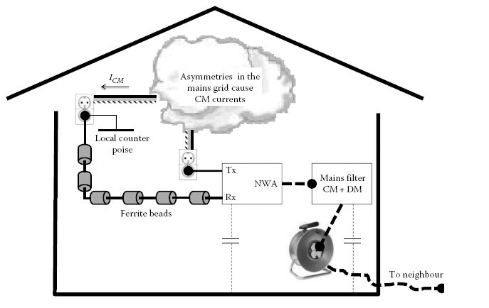
FIGURE 1.5
Private home with channel measurement equipment.

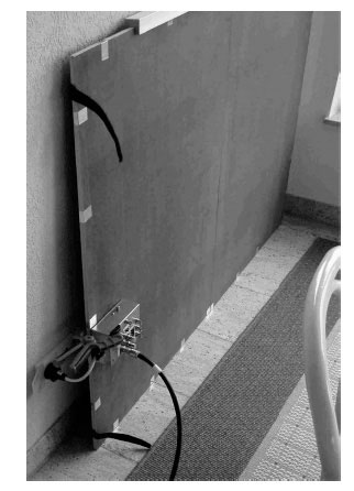
FIGURE 1.6
Ground plane with connected PLC coupler.

If the test instruments (namely the NWA) are connected to the mains section for electromagnetic interference (EMI), impedance and CTF measurements, the instruments represent an additional load and may cause measurement errors. Hence, whenever possible the power for the measurement equipment is drawn from a neighbouring flat via an extension cable. Further, on the right hand side of Figure 1.5, one can see a ‘mains filter CM+CD’. This filter is used to isolate the PE wire and consists of an isolation transformer and a line impedance stabilisation network (LISN). Additionally, a MIMO mains filter is used on each of the three wires eliminating DM signals, plus a CM choke to get rid of potential longitudinal signals. Such MIMO mains filter is not commercially available and was specifically manufactured for this measurement campaign.S₂₁ measurement results using this set-up may be found in Chapter 5.

1.4.2 Reflection Measurements and Input Impedance Calculation

The LV distribution network (LVDN) is a network with undefined complex characteristic impedance. The often measured absolute value of the input impedance has little practical significance. Adding a short piece of mains cable may change the results considerably. Thus, ETSI STF 410 measured the reflection loss expressed through the scattering parameter S₁₁ [60] at the ‘delta’ terminals of the couplers instead.

Generally, reflection measurement signals are fed and received at one and the same NWA port and require only the Tx coupler. The set-up is as shown in Figure 1.5 but without connecting the Rx coupler. The NWA is calibrated with a ‘short’, ‘open’ and a ‘50 Ω termination’ connected at the end of the coaxial cable. The MIMO PLC coupler is considered to be part of the PLC channel.

S₁₁ is a complex value which is a function of the load impedance and of the characteristic impedance of the measurement system (see Equation 1.14 for a general definition). Here, the measurement system consists of the NWA, which has a characteristic impedance of 50 Ω and the balun inside the MIMO coupler, which transforms the 50–200 Ω, that is, Z_coup = 200 Ω. Theoretically, S₁₁ on the 50 Ω side is identical to S₁₁ if measured on the 200 Ω side, except for a phase shift due to the length of the transmission lines inside the balun. The real and the imaginary parts of S₁₁ are recorded. For engineering purposes, the absolute value $| S_{11} |$ $| S_{11} |$ is often sufficient. It allows calculating the maximum line input impedance Z_{DM max}, that is,

$Z_{DM \max} = Z_{coup} \cdot \frac{(1 + | S_{11} |)}{(1 - | S_{11} |)} .$ $Z_{DM \max} = Z_{coup} \cdot \frac{(1 + | S_{11} |)}{(1 - | S_{11} |)} .$

(1.1)

However, the phase is also required to calculate Z_DM as a function of frequency and line length of the balun (≈0.3 m^-1) denoted x, that is,

$Z_{DM} = Z_{coup} \cdot \frac{(1 + S_{11} \cdot e^{j β x})}{(1 - S_{11} \cdot e^{^{j β x}})},$ $Z_{DM} = Z_{coup} \cdot \frac{(1 + S_{11} \cdot e^{j β x})}{(1 - S_{11} \cdot e^{^{j β x}})},$

(1.2)

where the phase constant β may be obtained as outlined in Appendix 1.A, Equation 1.12, assuming a wave speed v in the balun to be ≈200,000,000 m/s.

1.4.3 Noise Measurements

The noise measurement set-up is depicted in Figure 1.7. The MIMO coupler from Figure 1.4 is used in the star configuration (ports S1, S2, S3 and S4). Thus, the noise voltage present at the L, N and PE wires as well as the CM voltage can be directly sampled in the time domain by connecting a DSO (with digital signal processing [DSP] probe P1 to P4). The sampling rate is 500 Msamples/s. Further, care is taken that the DSP memory can store the four signals over 20 ms, corresponding to a single period of the AC line cycle at 50 Hz.

One drawback of the time domain measurement is that out-of-band noise can easily influence the result. Hence, DSO probes are using band-pass filters in order to reduce out-of-band noise. In each configuration, four different bands were tested, with the respective frequency ranges 2–100 MHz, 2–88 MHz, 30–100 MHz and 30–88 MHz. Further, in environments with low noise levels, low noise amplifiers are used to boost the input signal before recording. Each amplifier presented a flat frequency response up to 100 MHz and a gain of 28 dB.

FIGURE 1.7
Private home with noise measurement equipment.

1.5 Channel Characterisation and Modelling Approaches

The power line channel and noise situations heavily depend on the scenario as outlined in Section 1.2 and, hence, span a very large range. Generally, frequency-selective multi-path fading, a low-pass behaviour, AC-related cyclic short-term variations and abrupt long-term variations can be observed (see, for example, Chapters 2 through 5).

1.5.1 Channel Characteristics

Multi-path fading is caused by inhomogeneities of the power line segments where cabling and connected loads with different impedances give rise to signal reflections and in the sequel in-phase and anti-phase combinations of the arriving signal components. The corresponding transfer function can readily be derived in close form as infinite impulse response (IIR) filter [1] and underlying basics are outlined in Appendix 1.A. One important parameter capturing the frequency-selective characteristics is the rms delay spread (DS). For example, designing orthogonal frequency-division multiplexing (OFDM) systems, the guard interval might be chosen as 2–3 times the rms DS to deliver good system performance [61]. To provide an orientation, the mean of the observed rms DS for a band from 1 MHz up to 30 MHz in the MV, LV-access and LV-in-home situations in [21,61] was reported to be 1.9, 1.2 and 0.73 μs, respectively. Similarly, in Chapter 4, rms DS in the range 0.2–2.5 μs are reported from LV-in-home measurements performed within the 1.8–88 MHz frequency band.

Besides multi-path fading, the PLC channel exhibits time variation due to loads and/or line segments being connected or disconnected [62]. Further, through synchronising channel measurements with the electrical grid AC mains cycle, Cañete et al. were able to show that the in-home channel changes in a cyclostationary manner [47,63] (see also especially Chapters 2 and 21).

Until now, the low-pass behaviour of PLC channels has not been considered. It results from dielectric losses in the insulation between the conductors and is more pronounced in long cable segments such as outdoor underground cabling. Transfer function measurements on different cable types and for different length can be found in [6,25].

1.5.2 Channel Modelling Overview

Channel characterisation and modelling are tightly intervened. Channel characterisation in terms of channel measurements is indispensable to derive, validate and fine-tune channel models, while the channel models themselves often provide valuable understanding and insight that might stimulate more advanced channel characterisation.

In general, PLC channel models can be grouped into physical and parametric models (or into bottom-up and top-down models as in [7]). While physical models describe the electrical properties of a transmission line, for example, through the specification of cable type (line parameters), the cable length and the position of branches [48,64, 65, 66, 67] (see also Appendix 1.A), parametric models use a much higher level of abstraction from the physical reality and describe the channel, for example, through its impulse response or transfer function [25,68,69] (see also especially Chapters 4 and 5).

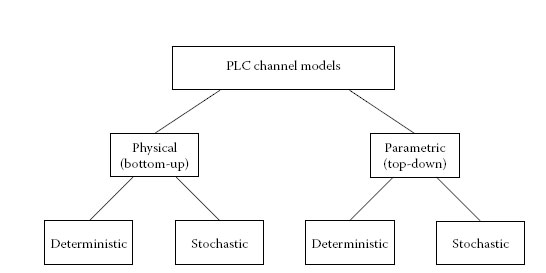
FIGURE 1.8
PLC channel modelling options.

Further, within each group, it can be distinguished between deterministic and stochastic models. While deterministic models aim at the description of one or a small set of specific reproducible PLC channels realisations, stochastic models aim at reflecting a wide range of channel realisations according to their probability of occurrence. This categorisation of channel modelling options is reflected in Figure 1.8 with a short description of each in the following.

Physical-deterministic modelling describes the electrical properties of a transmission line, for example, through the specification of cable parameters, cable length, the position of branches, etc. [64, 65, 66, 67,70]. Most physical models are based on representing power line elements and connected loads in the form of their ABCD or S-parameters [60], which are subsequently interconnected to produce the channel’s frequency response [64, 65, 66, 67,70, 71, 72, 73]. Alternatively, [1,74] introduced power line elements as well as connected loads as IIR filters, which is a novel and still intuitive approach if one considers that a communication signal travels in the form of an electromagnetic wave over the PLC channel and may bounce an infinite amount of times between neighbouring line discontinuities. Physical-deterministic models are especially well suited to represent and test deterministic power line situations. An introduction on to the underlying transmission line theory is provided in more detail in Appendix 1.A. MTL theory [42] is particularly well suited in the case of PLC propagation, since it allows describing the signal transmission along any arbitrary topology of interconnected wires and any set of connected loads. Physical-deterministic techniques are sometimes referred to as ‘bottom up’, as they start from a precise description of the electrical network under consideration in order to derive a global behaviour of the propagation channel. For a given electrical network, the physical-deterministic method can provide a CTF model very close to actual measurement. The drawback is that it requires a significant amount of input data and computational resources, especially if one wishes to derive channel statistics from a large number of different network topologies.

Physical-stochastic models combine the aforementioned deterministic approach with stochastic elements. In [75,76] a so-called ‘statistical bottom-up’ approach is presented, where the CTF is computed from the exact network topology using a deterministic algorithm. The stochastic nature of the model arises from the random generation of realistic electrical network topologies, based on a number of rules derived from observed cabling practices, an approach that has also been proposed in [1]. Physical stochastic models include the advantages of the deterministic approach in terms of accuracy with respect to physical transmission phenomena, while allowing for the random generation of statistically representative channel realisations. System engineers generally run digital simulations of the full system, which allow evaluating the behaviour and efficiency of different signal processing algorithms. A stochastic channel model is thus expected to reproduce the main effects of the propagation channel by generating a large number of random channel realisations, which are statistically representative of real-world observations.

Parametric-deterministic models are possibly one of the categories most used but not usually labelled as ‘parametric-deterministic’. Here, this label is referring to a database of measured parameters, such as the CTF, where simple playback of the measurement results can be used in PLC system simulations and performance studies. The advantage is that the exact parameters as observed in real situations are used without the risk to generate unrealistic channels due to modelling inaccuracies. On the other hand, a large and diverse database is needed to obtain meaningful results on a more general level. An example of such a huge database sourced from six European countries is documented in Chapter 5.

Parametric-stochastic models use a high level of abstraction and describe the channel, for example, through its impulse response characteristics [6,68,77]. The analysis of collected measurement data allows defining a model in the form of a mathematical expression. The mathematical form of the model is not necessarily linked to the physical phenomena taking place in the transmission of electromagnetic signals, but is designed to faithfully reproduce the main characteristics of the channel under study. The model parameters are defined in a statistical way, which allows generating different random realisations of the CTF (or the channel’s impulse response) exhibiting similar statistics as the experimental data. This modelling strategy is sometimes referred to as a ‘top-down’ approach, in the sense that it first considers global statistics of the propagation channel in order to define deeper details of the channel structure. This approach generally provides realistic results, with the drawback of requiring a large amount of experimental data to produce the model. The model in [25] is an early example of such statistical channel model, where a general CTF model has been defined based on physical considerations of the signal propagation through simple electrical network topologies. The model parameters were then obtained by fitting the mathematical model to a number of experimental measurements taken in the 0–20 MHz range. A more recent example of this modelling strategy is given in [78,79], where a channel model is defined on the basis of 144 measurements taken in different dwelling units in the 0–100 MHz range. The measurements are subdivided into nine different classes according to the observed channel capacity, and a statistical channel model is provided for each class.

Table 1.2 provides a comparison between the different PLC channel modelling options. Each of the four exists in its own right and bears advantages and disadvantages when it comes to specific applications. Thus, before deciding the type of channel model, the question What is the channel model supposed to do? is key. Some desirable properties of a channel model could, for example, be to

TABLE 1.2

Comparison of PLC Channel Modelling Options

Feature	Physical Deterministic	Physical Stochastic	Parametric Deterministic	Parametric Stochastic
Modelling principle	Electromagnetic transmission theory	Electromagnetic theory and topology generator	Playback of experimental measurement parameters	Statistical fit to experimental measurement parameters
Measurement requirements	None	None	Large data base	Large data base
Topology knowledge	Detailed	Detailed stochastic models	None	None
Complexity of model design	Medium	High	Low	Medium
Complexity of channel generation	High	High	Very low	Low
Correlated multi-user studies	Straightforward	Straightforward	Straightforward	Difficult
Closeness to experimental data	Accurate for considered topology	On a statistical basis	Exact	On a statistical basis
Ability to extrapolate	Yes	Yes	No	No

1. Describe the influence of the time-variant channel on the received signal quality in link and system simulations and algorithm testing, for example, on impulsive noise avoidance, signal-to-noise ratio estimation, channel filter tracking, MIMO schemes.

2. Model the correlation between temporal and spatial channel and noise variations.

3. Support the investigation of multi-point (multi-user) PLC systems.

4. Allow extension to various propagation scenarios based only on a small set of additional scenario measurements.

5. Describe modal coupling to be used in the design of MIMO couplers.

6. Assist in the development of the modem’s analogue front-end.

The objectives (1) to (3) and (5) can with more or less effort be realised with either a physical (bottom-up) or a parametric (top-down) model implementation. However, the objectives (4) and (6) are hard to realise with a parametric model. In general, parametric models require a larger range of measurement results to adjust the model parameters. On the contrary, physical models allow deploying knowledge, for example, on the physical dimensions of a new scenario, to adjust physical model parameters. Afterwards, only a smaller set of measurements is needed for rough verification purposes. Looking at signal processing–related issues with respect to MIMO PLC systems, a parametric model has certain advantages. It might be more easily deployed and parameters such as spatial correlation are well understood due to related studies in the wireless world [80]. However, looking at the practical implementation of, for example, MIMO couplers or the adjusting of analogue front-ends, a physical model, being significantly closer to the reality of electronic components, might be more useful. After these examples, it becomes clear that channel model selection has to be carried out on a case-by-case basis.

1.5.3 MIMO Channel Models

Turning specifically to MIMO channels, besides in the early patents [81, 82, 83, 84], one of the first public investigations of the MIMO access case appears in [85] with perfectly isolated multiple phase wires. Sparked also through the success of MIMO signal processing in the wireless world [41], larger public parametric-deterministic investigations of MIMO signal processing for BB in-home PLC appears in [86]. Similar evaluations, based on a limited set of measurements, are conducted in [87,88]. Following this trend, experimental channel and noise characterisation for MIMO PLC systems have been conducted in [47,89, 90, 91, 92]. For example, [87,88] conclude that the application of 2 × 2 MIMO signal processing to in-home PLC provides a capacity gain in the order of 1.9. Further, [86] showed that this capacity gain even increased with the number of Rx ports. In a 2 × 3 MIMO configuration, the average capacity gain ranged between 1.8 and 2.2 depending on the Tx power level. When adding CM reception, average gains between 2.1 and 2.6 were observed. Along these lines, additional MIMO capacity and throughput results can be found in Chapter 9.

Only a few proposals for physical-deterministic MIMO channel modelling have been made so far. The most straightforward bottom-up approach of modelling a channel composed of several wires is to apply MTL theory [42,60]. As shown in Figure 1.9, MTL theory can be applied to compute the currents i₁(x,t), i₂(x,t) and i₃(x,t) flowing in a three-wire transmission line as well as the corresponding differential voltages υ₁(x,t), υ₂(x,t) and υ₃(x,t) for a given line position x and a given time t To do so, a long list of per unit length line parameters needs to be known, that is, the inductances L₁₁, L₂₂ and L₃₃ and the resistances R₁₁, R₂₂ and R₃₃ of wires 1, 2 and 3, respectively, the mutual inductance between any pair of wires (L₁₂, L₁₃ and L₂₃), the capacitances (C₁₁, C₂₂ and C₃₃) and conductances (G₁₁, G₂₂ and G₃₃) of each wire with respect to the ground, the mutual capacitances (C₁₂, C₁₃ and C₂₃) and finally the conductances (G₁₂, G₁₃ and G₂₃) between any pair of wires. Note that some authors consider a simplified model with three conductors only, where the PE wire is assumed to be equivalent to the ground [93]. At high frequencies this assumption is not valid, especially when the reception of CM signals is expected as introduced in Figure 1.3. In such cases, a more complete model such as the one presented in Figure 1.9 is necessary to provide accurate results. The MTL modelling approach has been used in the work of Banwell and Galli for in-home LV electrical networks [48,66,94], and by Anatory et al. [73] for overhead MV or HV networks. However, these studies do not consider the use of three electrical wires for the purpose of MIMO communication.

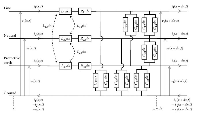
FIGURE 1.9
MTL theory: equivalent circuit of a per unit length section of a three-wire transmission line.

The first use of MTL theory to explicitly model a MIMO PLC channel in a physical-stochastic approach appears in [93,95]. The work therein extends the physical-stochastic SISO channel model presented in [76] by recomputing the MTL equations in the case of three conductors. Using the stochastic topology generator from [76], it is then possible to produce the CTF matrix for a large set of random electrical networks.

On the other hand, a parametric-stochastic approach has been applied by several research teams to devise models of the MIMO PLC channel. The first attempt is described in [96]. This study considers a 2 × 4 MIMO channel, where two differential input ports can be addressed simultaneously, and up to four Rx ports are considered, including the CM path. The model first considers a SISO PLC channel impulse response (CIR) composed of 5–20 taps according to the model defined within the European project OPERA [21]. It then builds the 2 × 4 MIMO channel matrix by producing eight variants of this CIR. Each of the variants has the same tap structure, but the amplitudes of some of these taps are multiplied using different random phases uniformly drawn from the interval [0,2π). The more taps are modified using a random phase shift, the more uncorrelated the channel becomes. The model produces MIMO channels that exhibit similar correlation values as observed in the measurements of [87]. The same approach is further developed in [97], where a 3 × 3 MIMO channel model has been designed to fit observations from a measurement campaign in France. In total, 42 3 × 3 MIMO channels were measured in five different houses using a vector NWA. The proposed MIMO channel model builds on the SISO channel model first defined by Zimmermann and Dostert [25], and later extended by Tonello by providing complementary channel statistics [98]. In the following, the notation adopted during the OMEGA project [99] will be used, where the CTF H(f) is given as a function of the frequency f by

$H (f) = A \sum_{p = 1}^{N_{p}} g_{p} e^{- j (2 π d_{p} / υ) f} e^{- (a_{0} + a_{1} f^{k}) d_{p}},$ $H (f) = A \sum_{p = 1}^{N_{p}} g_{p} e^{- j (2 π d_{p} / υ) f} e^{- (a_{0} + a_{1} f^{k}) d_{p}},$

(1.3)

where

υ represents the speed of the electromagnetic wave in the copper wire (which may be approximated as two-thirds the speed of light^*), that is, 200,000,000 m/s

d_p and g_p represent the length and gain of the propagation path

N_p represents the number of propagation paths

Parameters a₀, a₁, K and A are attenuation factors

FIGURE 1.10
Example of CTF simulated using the MIMO PLC channel model of Hashmat et al.[97]. Tx port D1 only.

An example of channel realisation is given in Figure 1.10 and the approach will be revisited in Chapter 5 to devise a novel channel model on the basis of European field measurements.

An alternative parametric-stochastic approach is presented in [100]. This study characterised the MIMO channel covariance matrix R_h, by analysing 96 MIMO channel measurements recorded in five houses in North America. Following a similar approach as in [80], the MIMO channel matrix H(f) is then modelled for each frequency f as

$H (f) = K (f) \cdot R_{r}^{1 / 2} (f) \cdot H^{'} (f) \cdot R_{t}^{1 / 2} (f),$ $H (f) = K (f) \cdot R_{r}^{1 / 2} (f) \cdot H^{'} (f) \cdot R_{t}^{1 / 2} (f),$

(1.4)

whrere

K(f) is a normalising constant

H’(f) is a channel matrix composed of independent and identically distributed complex Gaussian variables

R_r(f) and R_t(f) represent the Rx and Tx correlation matrices, respectively

Each channel correlation matrix is modelled by its decomposition in eigenvectors and eigenvalues. Details on this alternative model that allows very straightforward reproduction of the MIMO channel’s correlation properties can be found in Chapter 4.

1.6 Noise Characterisation and Modelling Approaches

Turning from the channel to the noise situation, one should note that in contrast to many other communication channels the noise in a power line channel cannot be described as additive white Gaussian noise (AWGN).

1.6.1 Noise Characteristics

The noise observed on indoor power line networks has been traditionally categorised into several classes, depending on its origin, its level and its time domain signature [101]. Power line noise can be grouped based on temporal as well as on spectral characteristics. Following, for example [5,6], one can distinguish coloured background noise, narrowband (NB) noise, periodic impulsive noise asynchronous to the mains frequency, periodic impulsive noise synchronous to the mains frequency and aperiodic impulsive noise as indicated in Figure 1.11.

A first class consists of the impulsive noise generated by electronic devices connected to the mains grid, such as switched mode power supplies, light dimmers or compact fluorescent lamps. This type of noise is of short duration (a few μs) but of relatively high level in the order of tens of mV. Due to the periodic nature of the mains, noisy devices can generate impulses in a synchronous way with the mains period. In this case, the impulsive noise is said to be periodic and synchronous to the mains frequency and presents a repetition rate at multiples of 50 or 60 Hz dependent on the mains frequency. Other noise sources generate impulses at a higher periodical rate up to several kHz, which are classified as periodic and asynchronous to the mains frequency. Finally, strong impulses can also be observed more sporadically, without any periodicity with the mains or with itself. This type of noise is sometimes referred to as aperiodic impulsive noise. Examples of such noise types recorded during field measurements are given in Chapter 5. The different characteristics of the impulsive noise have been statistically analysed through the observation of experimental data in [102]. A comprehensive model of the PLC impulsive noise has been proposed in [101]. The pulses are first statistically characterised in terms of amplitude, duration and repetition rate, and the global noise scenario is then modelled in the form of a Markov chain of noise states.

A second class of noise consists of narrowband (NB) noise. This type generally corresponds to ingress noise from broadcasting radio sources, in particular from the short-wave (SW) and frequency-modulation (FM) bands. Other ingress noise corresponds to leakages from nearby electrical or industrial equipment. This type of noise usually generates strong interference over long durations in a narrow frequency bandwidth in the order of tens of kHz.

FIGURE 1.11
Classification of PLC noise.

Finally, the remaining noise sources, presenting a lower level of interference, form a third class of noise called background noise. The background noise is generally coloured, in the sense that its power spectral density (PSD) is usually stronger at lower frequencies. In [30], the background noise PSD is modelled with decreasing power as a function of frequency. A similar approach has been adopted in the OMEGA Project [99], where the decaying function of frequency is complemented with a NB model representing the broadcast interference. Specifically, a statistical approach to average coloured background noise modelling is presented in [21] based on a large amount of noise measurements in MV as well as LV-access and LV-in-home situations. One general finding is that the mean noise power falls off exponentially with frequency. Alternatively, an interesting, quite different approach to model SISO PLC background noise is taken in [103], where a neural network technique is deployed for model generation.

An important feature relevant to all types of noise is their time dependency. Due to the uncontrolled nature of the noise source, the characteristics of the noise perceived at a given outlet can drastically change over time. For instance, the increase of human activity in the premises, for example, after working hours, leads to a stronger contribution of domestic appliances to the noise. It is less obvious that noise presents a cyclostationary structure, with a period related to the mains signal. This effect is mainly due to the periodic change of impedance at the network termination loads depending on the mains cycle. A thorough study of the time variation of the SISO PLC noise is presented in [104].

Further, Chapter 2 presents NB SISO noise measurement results for a small LV access network supplied by a single transformer substation. Beside the well-investigated noise classes, background and impulsive noise, a detailed look on the noise scenario identified two steady appearing noise classes: NB interferers and switched frequency noise (see Chapter 2 for details).

On the other hand, Chapter 3 introduces NB SISO (but multi-phase) noise measurements for typical underground LV access network in China. It is found that the noise power decreases with the frequency significantly. Measurements show a reduction of average noise power from a range between 50 and 90 dB μV at 50 kHz to a range between 30 and 60 dB μV at 500 kHz. Also, a considerable different noise level is reported at different times of the day.

1.6.2 Noise Modelling for MIMO PLC

Turning specifically to the MIMO noise situation, only a few modelling proposals have been made so far. For example, [89,105–107] are developing models of background noise on the basis of experimental noise measurements performed in five houses in France. The measurements were undertaken in the time domain using a DSO (as outlined previously in Section 1.4). However, the models are mainly targeting a reproduction of the frequency domain noise characteristics. In [106], the measurements are compared against two parametric SISO background noise models, namely, the Emsailian model [30] and the OMEGA model [99]. The models are fitted to the noise received on each of the MIMO Rx ports, and statistics of the model parameters are derived separately for each Rx port. In [107], the MIMO noise is regarded as a multi-variate time series (MTS), which allows capturing both the intrinsic characteristics of the noise received on each port, but also their cross-correlation. The noise MTS is then modelled using an autoregressive (AR) filtering procedure. The modelled noise PSD presents a high degree of similarity with the experimental observations. However, the model leaves room for improvements, especially considering its ability to reproduce sporadic time domain events, such as impulsive noise. Along the same lines, Chapter 5 presents MIMO noise measurements and noise modelling results. The measurements are conducted in 31 different dwelling units in five European countries, including Belgium, France, Germany, Spain and the United Kingdom. It was observed that the CM signal is affected on average by 5 dB more noise than the DM signals received on any wire combination. This difference can be explained by the higher sensitivity of the CM signal to interference from external sources, such as radio broadcasting. Moreover, it was observed that the L, PE and N ports present similar noise statistics. However, when considering large noise records (5% percentile), one can observe that the PE port is more sensitive to noise by ∼2 dB than the N or L ports. Similarly, for low noise levels (95% percentile), the L port is less sensitive to noise by ∼1 dB than the N or PE ports.

On the other hand, Chapter 4 addresses MIMO noise based on experimental measurements collected in the United States. In particular, it has been shown that the noise is correlated on the L-N, L-PE and N-PE receiver ports. The strongest correlation is measured between the L-PE and N-PE receiver ports. Moreover, the correlation is stronger for lower frequencies when compared to higher frequencies. Effects of noise correlation on MIMO capacity of a system with two transmit ports and three receive ports are studied. It is observed that noise correlation indeed helps to increase the MIMO channel capacity.

Besides all these initial efforts to characterise and model PLC noise specifically with respect to MIMO systems, a number of features of MIMO PLC noise still need to be investigated and modelled. In particular, the occurrence of impulsive noise, its time domain variations and the correlation of noise pulses observed on different Rx ports require further analysis.

1.7 Conclusion

MIMO PLC channel and noise characterisation and modelling have been introduced. As channel and noise are not independent of the deployed coupling strategies, these strategies have been covered in detail, specifically for LV in-home (or in building) configurations where a MIMO topology is formed by the live, neutral and protective earth wire. Various MIMO PLC transmitter and receiver topologies are possible. A major difference between transmitter and receiver side though is that CM injection is normally prevented at the transmitter, as CM signals are a direct cause of radiated emissions, which are limited by government regulations for obvious reasons. However, the power line channel does produce CM signals as a side effect because of asymmetry as well as parasitic capacitances. Thus at the receiver, the CM signal may as well be measured and processed for maximum receiver diversity and data throughput if receiver complexity is permissible.

Looking at characterisation and modelling, the characteristics of the SISO channel were presented citing a large amount of relevant literature. Two main modelling approaches, the physical (bottom-up) and the parametric (top-down) approaches, may be distinguished. Each approach may be paired with either deterministic or stochastic elements. In general, parametric models are based on series of field measurements and provide a compact description capturing the observed experimental characteristics. Physical models describe the underlying propagation phenomena in more detail. They are useful to predict the transmission conditions in a known environment or to launch physical-stochastic studies with the help of random topology generators.

With respect to SISO noise phenomena, important references in the field were cited capturing the main types of impairments. Impulsive noise consists of bursts of short-term over-voltage transients, which are generally considered in the time domain. NB noise and background noise are analysed in the frequency domain and correspond to long-term perturbations.

Due to the recent emergence of MIMO signal processing techniques for PLC systems, a few proposals only have been made so far to model the PLC MIMO channel and MIMO noise characteristics. The main existing studies in this field were reviewed and commented. The chapter’s intention was not to cover any characterisation or modelling approach in detail but rather to set the scene for the individual chapters on this topic. Specifically, Chapter 2 provides an approach for determining the link quality in a LV grid under the influence of the time-variant features of the NB transmission channel up to 500 kHz. Besides noise scenarios and CTF, there is a focus on the access impedances of the LV grid. Results obtained for a LV grid of a small university campus are presented.

Chapter 3 looks at the NB power line channel for LV access networks in China. Major channel characteristics such as access impedances, interferences and attenuations for frequencies between 30 and 500 kHz are evaluated based on measurement results in a typical urban underground network.

Chapter 4 deals with the characterisation of in-home MIMO power line channels and noise in the band from 1.8 to 88 MHz. The characterisation is based on channel measurements in multiple US homes. It focuses particularly on the spatial properties of the MIMO power line channel and introduces a parametric-stochastic MIMO channel model consistent with the measurements. Further, noise measurements are analysed for their spectral and correlation properties, which are shown to affect PLC MIMO capacity.

Chapter 5 takes a further step in the field of BB (1–100 MHz) LV in-home MIMO channel and noise characterisation and modelling. Novel parametric-stochastic models are derived based on a series of European measurements.

Appendix 1.A: Introduction to Transmission Line Theory

The following two subsections introduce a model for the dual conductor transmission line that is worth being familiar with before looking at MTL line theory as introduced in Section 1.5. Basic concepts from line parameters to propagation constant, characteristic impedance up to the physical (bottom-up) model of a dual conductor stub-line example network are described, showing how the concatenation of line segments leads to the multipath effects and in the sequel to frequency-selective fading.

1.A.1 Propagation Constant, Characteristic Impedance and Phase Velocity

The dual conductor transmission line can be described as a concatenation of lumped elements as displayed in Figure 1.12.R, L, G and C describe a shunt resistance per unit length (Ω/m), a series inductance per unit length (H/m), a shunt conductance per unit length (S/m) and a shunt capacitance per unit length (F/m), respectively. With the help of these lumped element parameters, also known as primary line parameters, the propagation constant γ and characteristic impedance Z₀ of the line can be calculated as shown later in this section.

FIGURE 1.12
Lumped elements transmission line representation.

The main function of the cables/conductors constituting the electrical grid is to deliver electricity. Hence, electrical cable manufactures usually do not specify line parameters in the frequency range of interest for PLC. Alternatively, the line parameters can be derived using electromagnetic theory as outlined in [29,108,109] and references therein. However, the math behind this direct approach is quite involved. Instead, different elec-tromagnetic simulation tools like [110,111] may be used to obtain the line parameters. In [108], the primary line parameters are derived as a function of the cable geometry, the experienced permittivity, permeability and conductivity. All but R are approximated as frequency independent.R is approximated proportional to the square root of the frequency of interest, that is, $R \propto \sqrt{f}$ $R \propto \sqrt{f}$ . The admittance G is further approximated as 0. Similarly, [6] describes the primary line parameters based on a specific cable geometry, permittivity, permeability and a dissipation factor. In contrast to [108], G is, however, described as a linear function of frequency. An extensive set of measurement-based primary line parameter models are given in [112] tailored to overhead LV power distribution networks. Finally, line parameters might be determined by measurements of the open-and short-circuited line input impedance as outlined in Appendix C of [108]. As an example, the line parameter values from [108] for dual conductor in-home cabling are reproduced in Table 1.3.

TABLE 1.3

Example Line Parameter Sets

Source: Based on Cañete Corripio, F.J., Caracterizacion y modelado de redes electricas interi-orescomo medio de transmision de banda ancha, Dissertation, Universidad de Malaga, Escuela Tecnica Superior de Ingenierya de Telecomunicacion, Malaga, Spain, 2006.

Starting with the lumped element representation of the transmission line, and using Krichhoff’s laws, the complex propagation constant γ can be derived from the wave equations in the frequency domain as in [60], that is,

$\begin{array}{l} γ = \sqrt{(R + j ω L) (G + j ω C)} \\ = α + j β, \end{array}$ $\begin{array}{l} γ = \sqrt{(R + j ω L) (G + j ω C)} \\ = α + j β, \end{array}$

(1.5)

where

ω is the angular frequency, that is, ω = 2π × f, and f is the frequency of interest

Re ${γ}$ ${γ}$ = α is the attenuation of the wave when travelling along the line, also known as attenuation constant, while Im ${γ}$ ${γ}$ = β represents the wave’s phase rotation, also called phase constant or wave number

γ, α and β have the unit 1/m

As β corresponds to phase rotation, its unit is sometimes expressed as rad/m

Under the condition of a low loss line, that is, G ≪ ωC∧R ≪ ωL, γ may be approximated as [6,60]

$\begin{array}{l} {γ|}_{low loss app} = j ω \sqrt{L C} (1 - \frac{j}{2} (\frac{R}{ω L} + \frac{G}{ω C})) \\ = j ω \sqrt{L C} + \frac{1}{2} (R \sqrt{\frac{C}{L}} + G \sqrt{\frac{L}{C}}) \end{array}$ $\begin{array}{l} {γ|}_{low loss app} = j ω \sqrt{L C} (1 - \frac{j}{2} (\frac{R}{ω L} + \frac{G}{ω C})) \\ = j ω \sqrt{L C} + \frac{1}{2} (R \sqrt{\frac{C}{L}} + G \sqrt{\frac{L}{C}}) \end{array}$

(1.6)

and thus

$α |_{low loss app} = \frac{1}{2} (R \sqrt{\frac{C}{L}} + G \sqrt{\frac{L}{C}}),$ $α |_{low loss app} = \frac{1}{2} (R \sqrt{\frac{C}{L}} + G \sqrt{\frac{L}{C}}),$

(1.7)

$β |_{low loss app} = ω \sqrt{L C} .$ $β |_{low loss app} = ω \sqrt{L C} .$

(1.8)

The line’s characteristic impedance Z₀ is of importance as it helps to specify the reflection and transmission coefficients that occur at line discontinuities, for example, when different line segments and loads are connected. On the basis of the wave equations, the characteristic line impedance as the ratio of voltages and currents on the line can be derived as in [60], that is,

$\begin{array}{l} Z_{0} = \frac{V_{0}^{+}}{I_{0}^{+}} \\ = \frac{- V_{0}^{-}}{I_{0}^{-}} \\ = \frac{R + j ω L}{γ} \\ = \sqrt{\frac{R + j ω L}{G + j ω C}}, \end{array}$ $\begin{array}{l} Z_{0} = \frac{V_{0}^{+}}{I_{0}^{+}} \\ = \frac{- V_{0}^{-}}{I_{0}^{-}} \\ = \frac{R + j ω L}{γ} \\ = \sqrt{\frac{R + j ω L}{G + j ω C}}, \end{array}$

(1.9)

where $V_{0}^{+}, I_{0}^{+}, V_{0}^{-}, I_{0}^{-}$ $V_{0}^{+}, I_{0}^{+}, V_{0}^{-}, I_{0}^{-}$ are the forward and backward travelling voltages and currents on the line, respectively. Also, Z₀ can under the low loss line approximation be simplified to [60]

$Z_{0} |_{low loss app} = \sqrt{\frac{L}{C}} .$ $Z_{0} |_{low loss app} = \sqrt{\frac{L}{C}} .$

(1.10)

Looking at the voltage wave in the time domain additionally allows to determine the wavelength and the phase velocity as [60]

$λ= \frac{2 π}{β}$ $λ= \frac{2 π}{β}$

(1.11)

and

$\begin{array}{l} υ = \frac{ω}{β} \\ = λ f, \end{array}$ $\begin{array}{l} υ = \frac{ω}{β} \\ = λ f, \end{array}$

(1.12)

which under the low loss line approximation with the help of Equation 1.8 simplifies to

$v |_{_{low loss app}} = \frac{1}{\sqrt{L C}} .$ $v |_{_{low loss app}} = \frac{1}{\sqrt{L C}} .$

(1.13)

1.A.2 Transmission Line Transfer Function

To understand the effects that lead to frequency-selective fading, consider the open stub line example in Figure 1.13 adapted from [77]. An impedance matched transmitter is placed at A. An impedance matched receiver is placed at C. Hence, in this simple example, there is no need to bother about impedance discontinuities at the input and the output of the network.D represents a 70 Ω parallel load.B marks the point of an electrical T-junction.l_x and Z_x represent the line lengths and characteristic impedances.t_xy indicates the transmission and r_xy the reflection coefficient encountered at impedance discontinuities whose dependencies on the characteristic impedances are derived in [60]. Generally, at an impedance discontinuity from Z_a to Z_b the reflection and transmission coefficients are given by

$r_{a b} = \frac{Z_{b} - Z_{a}}{Z_{b} + Z_{a}}$ $r_{a b} = \frac{Z_{b} - Z_{a}}{Z_{b} + Z_{a}}$

(1.14)

and

$t_{a b} = 1 + r_{a b} .$ $t_{a b} = 1 + r_{a b} .$

(1.15)

Specifically for the situation in Figure 1.13, r_1B is given by

$r_{1 B} = \frac{(Z_{2} | | Z_{3}) - Z_{1}}{(Z_{2} | | Z_{3}) + Z_{1}},$ $r_{1 B} = \frac{(Z_{2} | | Z_{3}) - Z_{1}}{(Z_{2} | | Z_{3}) + Z_{1}},$

(1.16)

where ( $Z_{2} | | Z_{3}$ $Z_{2} | | Z_{3}$ ) represents the impedance of Z₂ and Z₃ when connected in parallel.

FIGURE 1.13
Relationship of wave propagation and filter elements in the stub line example. (a–c) Represent wave propagation paths and (d–f) are the respective IIR-filter elements. (From Berger, L.T.and Moreno-Rodríguez, G., Acad. Publ.J. Commun., 4(1), 41. Copyright © 2009. Academy Publisher.)

A PLC signal travels in the form of a direct wave from A over B to C as displayed in Figure 1.13a. Another wave travels from A over B to D, bounces back to B and reaches C, as depicted in Figure 1.13b. All further waves travel from A to B, and undergo multiple bounces between B and D before they finally reach C (Figure 1.13c). The number of bounces between B and D is infinite, motivating the idea that an IIR filter may be used to represent the power line network. Considering the reflection and transmission coefficients as gains, and considering ideal transmission lines whose length relates only to a time delay, the simple stub line example may be transformed into IIR-filter elements as displayed in Figure 1.13d–f, where the boxes represent delays and the triangles represent filter coefficients.

The complete filter obtained for the stub line example is displayed in Figure 1.14 in its more conventional canonical form. A discrete time representation is considered. The smallest time step T_s relates to the system’s sampling frequency via f_s = 1/T_s. Thus, every line length relates to a delay which, measured in samples, can be expressed as

$\begin{array}{l} N_{delay, x} = \frac{{delay}_{x}}{T_{s}} \\ = \frac{l_{x}}{T_{s} \cdot υ_{x}}, \end{array}$ $\begin{array}{l} N_{delay, x} = \frac{{delay}_{x}}{T_{s}} \\ = \frac{l_{x}}{T_{s} \cdot υ_{x}}, \end{array}$

(1.17)

where l_x and υ_x represent the length and the wave speed of line x, respectively (∼200,000,000 m/s). The filter from Figure 1.14 may then be expressed through its z-transfer function where a time delay is given as $z^{- Round {l_{x} / T_{s} . v_{x}}}$ $z^{- Round {l_{x} / T_{s} . v_{x}}}$ . Round ${\cdot}$ ${\cdot}$ stands for rounding to the nearest integer. Instead of using this lengthy notation, the z-transform of the time delay caused by line length l_x is denoted by z^−l_k. The z-transfer functions of the sub-filter blocks marked in Figure 1.14 as H_a, H_b and H_c are

FIGURE 1.14
IIR-filter representation of stub line example. (From Berger, L.T.and Moreno-Rodríguez, G., Acad. Publ.J. Commun., 4(1), 41. Copyright © 2009. Academy Publisher.)

$H_{a} = t_{1 B} \cdot z^{- l_{1}},$ $H_{a} = t_{1 B} \cdot z^{- l_{1}},$

(1.18)

$H_{b} = 1 + \frac{t_{3 B} \cdot r_{3 D} \cdot z^{- 2 l_{3}}}{1 - r_{3 B} \cdot r_{3 D} \cdot z^{- 2 l_{3}}},$ $H_{b} = 1 + \frac{t_{3 B} \cdot r_{3 D} \cdot z^{- 2 l_{3}}}{1 - r_{3 B} \cdot r_{3 D} \cdot z^{- 2 l_{3}}},$

(1.19)

$H_{c} = z^{- l_{2}} .$ $H_{c} = z^{- l_{2}} .$

(1.20)

The overall z-transfer function of the stub line example is obtained through the concatenation of the three sub-filter blocks:

$\begin{array}{l} H = H_{a} \cdot H_{b} \cdot H_{c} \\ = t_{1 B} \cdot z^{- l_{1}} . (1 + \frac{t_{3 B} \cdot r_{3 D} \cdot z^{- 2 l_{3}}}{1 - r_{3 B} \cdot r_{3 D} \cdot z^{- 2 l_{3}}}) \cdot z^{- l_{2}} \\ = \frac{t_{1 B} \cdot z^{- (l_{1} + l_{2})}}{1 - r_{3 B} \cdot r_{3 D} \cdot z^{- 2 l_{3}}} + \frac{(t_{3 B} - r_{3 B}) \cdot r_{3 D} \cdot t_{1 B} \cdot z^{- (l_{1} + l_{2} + 2 l_{3})}}{1 - r_{3 B} \cdot r_{3 D} \cdot z^{- 2 l_{3}}} . \end{array}$ $\begin{array}{l} H = H_{a} \cdot H_{b} \cdot H_{c} \\ = t_{1 B} \cdot z^{- l_{1}} . (1 + \frac{t_{3 B} \cdot r_{3 D} \cdot z^{- 2 l_{3}}}{1 - r_{3 B} \cdot r_{3 D} \cdot z^{- 2 l_{3}}}) \cdot z^{- l_{2}} \\ = \frac{t_{1 B} \cdot z^{- (l_{1} + l_{2})}}{1 - r_{3 B} \cdot r_{3 D} \cdot z^{- 2 l_{3}}} + \frac{(t_{3 B} - r_{3 B}) \cdot r_{3 D} \cdot t_{1 B} \cdot z^{- (l_{1} + l_{2} + 2 l_{3})}}{1 - r_{3 B} \cdot r_{3 D} \cdot z^{- 2 l_{3}}} . \end{array}$

(1.21)

The derived H is the through-forward filter of the stub line from input A to output B. Further detailed derivations of elements like a star junction or a general load can be found in [1]. It becomes clear that although accurate, this type of physical (bottom-up) modelling can become mathematically quite involved, especially when considering MTL lines. Nevertheless, it serves as an interesting example to understand the processes that lead to multi-path propagation and in the sequel frequency-selective fading of the PLC channel.

Acknowledgements

The work has been partially supported by the Spanish Ministry of Science and Innovation (MICINN) Program INNCORPORA-Torres Quevedo 2011. Much gratitude also goes to ETSI, the experts participating in STF 410 and all volunteers supporting the MIMO PLC field measurements.

References

1. L. T. Berger and G. Moreno-Rodríguez, Power line communication channel modelling through concatenated IIR-filter elements, Academy Publisher Journal of Communications, 4(1), 41–51, February 2009.

2. L. T. Berger, Broadband powerline communications, in Convergence of Mobile and Stationary Next Generation Networks, K. Iniewski, Ed. John Wiley & Sons, Hoboken, NJ, 2010, ch. 10, pp. 289–316.

3. L. T. Berger, Wireline communications in smart grids, in Smart Grid – Applications, Communications and Security, L. T. Berger and K. Iniewski, Eds. John Wiley & Sons, Hoboken, NJ, April 2012, pp. 191–230.

4. L. T. Berger, A. Schwager and J. J. Escudero-Garzás, Power line communications for smart grid applications, Hindawi Publishing Corporation Journal of Electrical and Computer Engineering, no. ID 712376, pp. 1–16, 2013, Received 3 August 2012; Accepted 29 December 2012, Academic Editor: Ahmed Zeddam. [Online] Available: http://www.hindawi.com/journals/jece/aip/712376/.

5. M. Zimmermann and K. Dostert, An analysis of the broadband noise scenario in power-line networks, in International Symposium on Power Line Communications and Its Applications (ISPLC), Limerick, Ireland, April 2000, pp. 131–138.

6. M. Babic, M. Hagenau, K. Dostert and J. Bausch, Theoretical postulation of PLC channel model, The OPERA Consortium, IST Integrated Project Deliverable D4v2.0, March 2005.

7. E. Biglieri, Coding and modulation for a horrible channel, IEEE Communications Magazine, 41(5), 92–98, May 2003.

8. International Telecommunications Union (ITU), ITU radio regulations. [Online] Available: http://life.itu.int/radioclub/rr/art02.htm (accessed March 2013), 2008, Vol. 1, Article 2; Edition of 2008.

9. S. Galli, A. Scaglione and Z. Wang, For the grid and through the grid: The role of power line communications in the smart grid, Proceedings of the IEEE, 99(6), June 2011.

10. K. Dostert, Powerline Communications. Prentice Hall, Upper Saddle River, NJ, 2001.

11. G. Held, Understanding Broadband over Power Line. CRC Press, Boca Raton, FL, 2006.

12. P. Sobotka, R. Taylor and K. Iniewski, Broadband over power line communications: Home networking, broadband access, and smart power grids, in Internet Networks: Wired, Wireless, and Optical Technologies, ser. Devices, Circuits, and Systems, K. Iniewski, Ed., CRC Press, Boca Raton, FL, December 2009, ch. 8.

13. R. Pighi and R. Raheli, On multicarrier signal transmission for high voltage power lines, in IEEE International Symposium on Power Line Communications and its Applications (ISPLC), Vancouver, British Columbia, Canada, April 2005.

14. D. Hyun and Y. Lee, A study on the compound communication network over the high voltage power line for distribution automation system, in International Conference on Information Security and Assurance (ISA), Busan, Korea, April 2008, pp. 410–414.

15. R. Aquilu, I. G. J. Pijoan and G. Sanchez, High-voltage multicarrier spread-spectrum system field test, IEEE Transactions on Power Delivery, 24(3), 1112–1121, July 2009.

16. N. Strandberg and N. Sadan, HV-BPL phase 2 field test report, U.S. Department of Energy, Technical Report DOE/NETL-2009/1388, 2009, http://www.netl.doe.gov/smartgrid/refer-enceshelf/reports/HV-BPL_Final_Report.pdf (accessed December 2010).

17. P. Wouters, P. van der Wielen, J. Veen, P. Wagenaars and E. Steennis, Effect of cable load impedance on coupling schemes for MV power line communication, IEEE Transactions on Power Delivery, 20(2), 638–645, April 2005.

18. R. Benato and R. Caldon, Application of PLC for the control and the protection of future distribution networks, in IEEE International Symposium on Power Line Communications and Its Applications (ISPLC), Pisa, Italy, March 2007.

19. A. Cataliotti, A. Daidone and G. Tiné, Power line communication in medium voltage systems: Characterization of MV cables, IEEE Transactions on Power Delivery, 23(4), 1896–1902, October 2008.

20. N. Pine and S. Choe, Modified multipath model for broadband MIMO power line communications, in IEEE International Symposium on Power Line Communications and Its Applications, Beijing, China, April 2012.

21. P. Meier, M. Bittner, H. Widmer, J. -L. Bermudez, A. Vukicevic, M. Rubinstein, F. Rachidi, M. Babic and J. Simon Miravalles, Pathloss as a function of frequency, distance and network topology for various LV and MV European powerline networks, The OPERA Consortium, Project Deliverable, EC/IST FP6 Project No. 507667 D5v0.9, April 2005.

22. A. Rubinstein, F. Rachidi, M. Rubinstein, A. Vukicevic, K. Sheshyekani, W. Bschelin and C. Rodríguez-Morcillo, EMC guidelines, The OPERA Consortium, IST Integrated Project Deliverable D9v1.1, October 2008, IST Integrated Project No. 026920.

23. A. Vukicevic, Electromagnetic compatibility of power line communication systems, Dissertation, École Polytechnique Fédérale de Lausanne, Lausanne, Switzerland, June 2008, no. 4094.

24. N. Gonzáez-Prelcic, C. Mosquera, N. Degara and A. Currais, A channel model for the Galician low voltage mains network, in International Symposium on Power Line Communications (ISPLC), Malmö, Sweden, March 2001, pp. 365–370.

25. M. Zimmermann and K. Dostert, A multipath model for the powerline channel, IEEE Transactions on Communications, 50(4), 553–559, April 2002.

26. H. Liu, J. Song, B. Zhao and X. Li, Channel study for medium-voltage power networks, in IEEE International Symposium on Power Line Communications (ISPLC), Orlando, FL, March 2006, pp.245–250.

27. H. Philipps, Performance measurements of powerline channels at high frequencies, in International Symposium in Power Line Communications, Tokyo, Japan, March 1998, pp. 229–237.

28. D. Liu, E. Flint, B. Gaucher and Y. Kwark, Wide band AC power line characterization, IEEE Transactions on Consumer Electronics, 45(4), 1087–1097, 1999.

29. H. Philipps, Hausinterne Stromversorgungsnetze als übertragungswege für hochratige digitale Signale, Dissertation, Technical University Carolo-Wilhelmina zu Braunschweig, Braunschweig, Germany, 2002.

30. T. Esmailian, F. R. Kschischang and P. G. Gulak, In-building power lines as high-speed communication channels: Channel characterization and a test channel ensemble, International Journal of Communication Systems, 16, 381–400, 2003.

31. ETSI Technical Committee PowerLine Telecommunication (PLT), PowerLine Telecommunications (PLT); Hidden Node review and statistical analysis, Technical Report TR 102 269 V1.1.1, December 2003.

32. A. Schwager, L. Stadelmeier and M. Zumkeller, Potential of broadband power line home networking, in Second IEEE Consumer Communications and Networking Conference, January 2005, pp. 359–363.

33. P. Karols, K. Dostert, G. Griepentrog and S. Huettinger, Mass transit power traction networks as communication channels, IEEE Journal on Selected Areas in Communications, 24(7), 1339–1350, July 2006.

34. T. Huck, J. Schirmer, T. Hogenmuller and K. Dostert, Tutorial about the implementation of a vehicular high speed communication system, in International Symposium on Power Line Communications and Its Applications (ISPLC), Vancouver, British Columbia, Canada, April 2005, pp. 162–166.

35. S. Galli, T. Banwell and D. Waring, Power line based LAN on board the NASA space shuttle, in IEEE 59th Vehicular Technology Conference, Milan, Italy, Vol. 2, May 2004, pp. 970–974.

36. J. Wolf, Power line communication (PLC) in space – Current status and outlook, in ESA Workshop on Aerospace EMC, Venice, Italy, 2012, pp. 1–6.

37. S. Tsuzuki, M. Yoshida and Y. Yamada, Characteristics of power-line channels in cargo ships, in International Symposium on Power Line Communications and Its Applications (ISPLC), Pisa, Italy, March 2007, pp. 324–329.

38. J. Yazdani, K. Glanville and P. Clarke, Modelling, developing and implementing sub-sea power-line communications networks, in International Symposium on Power Line Communications and Its Applications, Vancouver, British Columbia, Canada, 2005, pp. 310–316

39. L. T. Berger and K. Iniewski, Smart Grid – Applications, Communications and Security. John Wiley & Sons, New York, April 2012.

40. G. J. Foschini and M. J. Gans, On limits of wireless communications in a fading environment when using multiple antennas, Wireless Personal Communications, (6), 311–335, 1998.

41. L. Schumacher, L. T. Berger and J. Ramiro Moreno, Recent advances in propagation characterisation and multiple antenna processing in the 3GPP framework, in XXVIth URSI General Assembly, Maastricht, the Netherlands, August 2002, session C2.

42. C. R. Paul, Analysis of Multiconductor Transmission Lines. John Wiley & Sons, New York, 1994.

43. European Telecommunication Standards Institute (ETSI), Powerline Telecommunications (PLT); MIMO PLT; Part 1: Measurement Methods of MIMO PLT, February 2012. [Online] Available: http://www.etsi.org/deliver/etsi_tr/101500_101599/10156201/01.03.01_60/tr_10156201v010301p.pdf.

44. International Electrotechnical Commission (IEC), Power line communication system or power utility applications – Part 1: Planning of analog and digital power line carrier systems operating over EHV/HV/MV electricity grids, September 2012.

45. ETSI Technical Committee PowerLine Telecommunication (PLT), PowerLine Telecommunication (PLT); Basic data relating to LVDN measurements in the 3 MHz to 100 MHz frequency range, Technical Report TR 102 370 V1.1.1, November 2004. [Online] Available: http://www.etsi.org/deliver/etsi_tr/102300_102399/102370/01.01.01_60/.

46. European Telecommunication Standards Institute (ETSI), Powerline Telecommunications (PLT); MIMO PLT Universal Coupler, Operating Instructions – Description, May 2011. [Online] Available: http://www.etsi.org/deliver/etsi_tr/101500_101599/101562/01.01.01_60/tr_101562v010101p.pdf.

47. A. Schwager, Powerline communications: Significant technologies to become ready for integration, Dissertation, Universität Duisburg-Essen, Fakultät für Ingenieurwissenschaften, Duisburg-Essen, Germany, 2010. [Online] Available: http://duepublico.uni-duisburg-essen.de/servlets/DerivateServlet/Derivate-24381/Schwager_Andreas_Diss.pdf.

48. T. Banwell and S. Galli, A novel approach to the modeling of the indoor power line channel part I: Circuit analysis and companion model, IEEE Transactions on Power Delivery, 20(2), 655–663, April 2005.

49. M. Ishihara, D. Umehara and Y. Morihiro, The correlation between radiated emissions and power line network components on indoor power line communications, in IEEE International Symposium on Power Line Communications and Its Applications, Orlando, FL, 2006, pp. 314–318.

50. M. Tanaka, High frequency noise power spectrum, impedance and transmission loss of power line in Japan on intrabuilding power line communications, IEEE Transactions on Consumer Electronics, (CE-34), 321–326, May 1988.

51. S. Tsuzuki, S. Yamamoto, T. Takamatsu and Y. Yamada, Measurement of Japanese indoor power-line channel, in Fifth International Symposium Power-Line Communications, Malmö, Sweden, 2001, pp. 79–84.

52. J. A. Malack and J. R. Engstrom, RF impedance of United States and European power lines, IEEE Transactions on Electromagnetic Compatibility, EMC-18, 36–38, February 1976.

53. J. R. Nicholson and J. A. Malack, RF impedance of power lines and line impedance stabilization networks in conducted interference measurements, IEEE Transactions on Electromagnetic Compatibility, EMC-15, 84–86, May 1973.

54. Ministry of Internal Affairs and Communications (MIC), Report of the CISPR committee, the information and communication council, June 2006, available only in Japanese. [Online] Available: http://www.soumu.go.jp/joho_tsusin/policyreports/joho_tsusin/bunkakai/pdf/060629_3_1-2.pdf.

55. M. Hove, T. O. Sanya, A. J. Snyders, I. R. Jandrell and H. C. Ferreira, The effect of type of transient voltage suppressor on the signal response of a coupling circuit for power line communications, in IEEE AFRICON, Livingstone, Zambia, 2011, pp. 1–6.

56. G. R. and S. K. Das, Power line transient interference and mitigation techniques, in IEEE INCEMIC, Chennai, India, 2003, pp. 147–154.

57. N. Mungkung, S. Wongcharoen, C. Sukkongwari and S. Arunrungrasmi, Design of AC electronics load surge protection, International Journal of Electrical, Computer and Systems Engineering, 1(2), 126–131, 2007.

58. Littlefuse, Combining GDTs and MOVs for surge protection of AC power lines, application Note EC640. [Online] Available: www.littelfuse.com.

59. ETSI Technical Committee PowerLine Telecommunication (PLT), Power line telecommunications (PLT); Channel characterization and measurement methods, Technical Report TR 102 175 V1.1.1, 2003. [Online] Available: http://www.etsi.org/deliver/etsi_tr/102100_102199/102175/01.01.01_60/tr_102175v010101p.pdf.

60. D. M. Pozar, Microwave Engineering, 3rd edn. John Wiley & Sons, New York, 2005.

61. S. Galli, A simplified model for the indoor power line channel, in IEEE International Symposium on Power Line Communications and Its Applications (ISPLC), Dresden, Germany, March 2009, pp. 13–19.

62. F. J. Cañete Corripio, L. Díez del Río and J. T. Entrambasaguas Muñoz, A time variant model for indoor power-line channels, in International Symposium on Power Line Communications (ISPLC), Malmö, Sweden, March 2001, pp. 85–90.

63. F. J. Cañete, L. Dİez, J. A. Cortés and J. T. Entrambasaguas, Broadband modelling of indoor power-line channels, IEEE Transactions on Consumer Electronics, 48(1), 175–183, February 2002.

64. T. Esmailian, F. R. Kschischang and P. G. Gulak, An in-building power line channel simulator, in International Symposium on Power Line Communications and Its Applications (ISPLC), Athens, Greece, March 2002.

65. F. J. Cañete, J. A. Cortés, L. Díez and J. T. Entrambasaguas, Modeling and evaluation of the indoor power line transmission medium, IEEE Communications Magazine, 41(4), 41–47, April 2003.

66. S. Galli and T. Banwell, A novel approach to the modeling of the indoor power line channel – Part II: Transfer function and its properties, IEEE Transactions on Power Delivery, 20(3), 1869–1878, July 2005.

67. T. Sartenaer and P. Delogne, Deterministic modeling of the (shielded) outdoor power line channel based on the multiconductor transmission line equations, IEEE Journal on Selected Areas in Communications, 24(7), 1277–1291, July 2006.

68. H. Philipps, Development of a statistical model for powerline communication channels, in International Symposium on Power Line Communications (ISPLC), Limerick, Ireland, April 2000, pp.153–160.

69. J. -H. Lee, J. -H. Park, H. -S. Lee, G. -W. Lee and S. -C. Kim, Measurement, modelling and simulation of power line channel for indoor high-speed data communications, in International Symposium on Power Line Communications (ISPLC), Malmö, Sweden, March 2001, pp. 143–148.

70. S. Barmada, A. Musolino and M. Raugi, Innovative model for time-varying power line communication channel response evaluation, IEEE Journal on Selected Areas in Communications, 7(24), 1317–1326, July 2006.

71. S. Galli and T. C. Banwell, A deterministic frequency-domain model for the indoor power line transfer function, IEEE Journal on Selected Areas in Communications, 24(7), 1304–1316, July 2006.

72. J. Anatory, N. Theethayi and R. Thottappillil, Power-line communication channel model for interconnected networks – Part I: Two-conductor system, IEEE Transactions on Power Delivery, 24(1), 118–123, January 2009.

73. J. Anatory, N. Theethayi and R. Thottappillil, Power-line communication channel model for interconnected networks – Part II: Multiconductor system, IEEE Transactions on Power Delivery, 24, 124–128, January 2009.

74. G. Moreno-Rodríguez and L. T. Berger, An IIR-filter approach to time variant PLC-channel modelling, in IEEE International Symposium on Power Line Communications and Its Applications (ISPLC), Jeju, South Korea, April 2008, pp. 87–92.

75. A. M. Tonello and F. Versolatto, Bottom-up statistical PLC channel modeling – Part II: Inferring the statistics, IEEE Transactions on Power Delivery, 25(4), 2356–2363, October 2010.

76. A. M. Tonello and F. Versolatto, Bottom-up statistical PLC channel modeling – Part I: Random topology model and efficient transfer function computation, IEEE Transactions on Power Delivery, 26(2), 891–898, April 2011.

77. M. Zimmermann and K. Dostert, A multi-path signal propagation model for the power line channel in the high frequency range, in International Symposium on Power-Line Communications and its Applications (ISPLC), Lancaster, U.K., April 1999, pp. 45–51.

78. M. Tlich, A. Zeddam, F. Moulin and F. Gauthier, Indoor power line communications channel characterization up to 100 MHz – Part I: One-parameter deterministic model, IEEE Transactions on Power Delivery, 23(3), 1392–1401, July 2008.

79. M. Tlich, A. Zeddam, F. Moulin and F. Gauthier, Indoor power line communications channel characterization up to 100 MHz – Part II: Time-frequency analysis, IEEE Transactions on Power Delivery, 23(3), 1402–1409, July 2008.

80. J. P. Kermoal, L. Schumacher, K. I. Pedersen, P. E. Mogensen and F. Frederiksen, A stochastic MIMO radio channel model with experimental validation, IEEE Journal on Selected Areas in Communications, 20, (6), 1211–1226, August 2002.

81. C. S. Cowies and J. P. Leveille, Modal transmission method and apparatus for multi-conductor wireline cables, Patent EP 0 352 869 A2, January, 1990. [Online] Available: http://worldwide.espacenet.com/espacenetDocument.pdf?flavour=trueFull&locale=es_LP&FT=D&date=19900131&CC=EP&NR=0352869A2&KC=A2&popup=true, accessed October 2012.

82. J. Dagher, System and method for transporting high-bandwidth signals over electrically conducting transmission lines, Patent US 5 553 097 A, September 1996. [Online] Available: http://worldwide.espacenet.com/espacenetDocument.pdf?flavour=trueFull&locale=es_LP&FT=D&date=19960903&CC=US&NR=5553097A&KC=A&popup=true, accessed October 2012.

83. D. C. Mansur, Eigen-mode encoding of signals in a data group, Patent US 6 226 330 B1, May 2001. [Online] Available: http://worldwide.espacenet.com/espacenetDocument.pdf?flavour=trueFull&locale=es_LP&FT=D&date=20010501&CC=US&NR=6226330B1&KC=B1&popup=true, accessed October 2012.

84. B. Honary, J. Yazdani and P. A. Brown, Space time coded data transmission via inductive effect between adjacent power lines, Patent GB2 383 724, December 2001. [Online] Available: http://worldwide.espacenet.com/publicationDetails/biblio?DB=EPODOC&II=0&ND=3&adjacent=true&locale=en_EP&FT=D&date=20030702&CC=GB&NR=2383724A&KC=A, accessed October 2012.

85. C. L. Giovaneli, J. Yazdani, P. Farrell and B. Honary, Application of space-time diversity/coding for power line channels, in International Symposium on Power Line Communications and Its Applications (ISPLC), Athens, Greece, March 2002.

86. L. Stadelmeier, D. Schill, A. Schwager, D. Schneider and J. Speidel, MIMO for inhome power line communications, in Seventh International ITG Conference on Source and Channel Coding (SCC), Ulm, Germany, January 2008.

87. R. Hashmat, P. Pagani and T. Chonavel, MIMO capacity of inhome PLC links up to 100 MHz, in Third Workshop on Power Line Communications, Udine, Italy, October 2009.

88. R. Hashmat, P. Pagani and T. Chonavel, MIMO communications for inhome PLC networks: Measurements and results up to 100 MHz, in IEEE International Symposium on Power Line Communications and Its Applications, Rio de Janeiro, Brazil, March 2010.

89. R. Hashmat, P. Pagani, A. Zeddam and T. Chonavel, Measurement and analysis of inhome MIMO PLC channel noise, in Fourth Workshop on Power Line Communications, Boppard, Germany, September 2010.

90. D. Veronesi, R. Riva, P. Bisaglia, F. Osnato, K. Afkhamie, A. Nayagam, D. Rende and L. Yonge, Characterization of in-home MIMO power line channels, in 2011 IEEE International Symposium on Power Line Communications and Its Applications (ISPLC), April 2011, pp. 42–47.

91. D. Rende, A. Nayagam, K. Afkhamie, L. Yonge, R. Riva, D. Veronesi, F. Osnato and P. Bisaglia, Noise correlation and its effects on capacity of inhome MIMO power line channels, in IEEE International Symposium on Power Line Communications, Udine, Italy, April 2011, pp. 60–65.

92. D. Schneider, A. Schwager, W. Baschlin and P. Pagani, European MIMO PLC field measurements: Channel analysis, in 2012 16th IEEE International Symposium on Power Line Communications and Its Applications (ISPLC), Beijing, China, March 2012, pp. 304–309.

93. F. Versolatto and A. M. Tonello, MIMO PLC random channel generator and capacity analysis, in IEEE International Symposium on Power Line Communications and Its Applications, Udine, Italy, April 2011, pp. 66–71.

94. T. Banwell, Accurate indoor residential PLC model suitable for channel and EMC estimation, in IEEE 6th Workshop on Signal Processing Advances in Wireless Communications, New York, June 2005, pp. 985–990.

95. F. Versolatto and A. M. Tonello, An MTL theory approach for the simulation of MIMO power-line communication channels, IEEE Transactions on Power Delivery, 26(3), 1710–1717, July 2011.

96. A. Canova, N. Benvenuto and P. Bisaglia, Receivers for MIMO-PLC channels: Throughput comparison, in IEEE International Symposium on Power Line Communications and Its Applications, Rio, Brazil, March 2010.

97. R. Hashmat, P. Pagani, A. Zeddam and T. Chonave, A channel model for multiple input multiple output in-home power line networks, in 2011 IEEE International Symposium on Power Line Communications and Its Applications (ISPLC), Udine, Italy, April 2011, pp. 35–41.

98. A. M. Tonello, Wideband impulse modulation and receiver algorithms for multiuser power line communications, EURASIP Journal on Advances in Signal Processing, 1–14, 2007.

99. M. Tlich, P. Pagani, G. Avril, F. Gauthier, A. Zeddam, A. Kartit, O. Isson et al., PLC channel characterization and modelling, OMEGA, European Union Project Deliverable D3.2 v.1.2 IST Integrated Project No ICT-213311, February 2011. [Online] Available: http://www.ict-omega.eu/publications/deliverables.html (accessed April 2013).

100. A. Tomasoni, R. Riva and S. Bellini, Spatial correlation analysis and model for in-home MIMO power line channels, in IEEE International Symposium on Power Line Communications and Its Applications, Beijing, China, April 2012.

101. M. Zimmermann and K. Dostert, Analysis and modeling of impulsive noise in broad-band powerline communications, IEEE Transactions on Electromagnetic Compatibility, 44(1), 249–258, February 2002

102. V. Degardin, M. Lienard, A. Zeddam, F. Gauthier and P. Degauque, Classification and characterization of impulsive noise on indoor power lines used for data communications, IEEE Transactions on Consumer Electronics, 48(4), 913–918, November 2002.

103. Y.-T. Ma, K.-H. Liu, Z.-J. Zhang, J.-X. Yu and X.-L. Gong, Modeling the colored background noise of power line communication channel based on artificial neural network, in Wireless and Optical Communications Conference, Shanghai, China, May 2010.

104. J. A. Cortés, L. Dİez, F. J. Cañete and J. J. Sánchez-Martínez, Analysis of the indoor broadband power line noise scenario, IEEE Transactions on Electromagnetic Compatibility, 52(4), 849–858, November 2010

105 P. Pagani, R. Hashmat, A. Schwager, D. Schneider and W. Baschlin, European MIMO PLC field measurements: Noise analysis, in 2012 16th IEEE International Symposium on Power Line Communications and Its Applications (ISPLC), Beijing, China, March 2012, pp. 310–315.

106. R. Hashmat, P. Pagani, T. Chonavel and A. Zeddam, Analysis and modeling of background noise for inhome MIMO PLC channels, in IEEE International Symposium on Power Line Communications and its Applications, Beijing, China, March 2012.

107. R. Hashmat, P. Pagani, T. Chonavel and A. Zeddam, A time domain model of background noise for inhome MIMO PLC networks, IEEE Transactions on Power Delivery, 27(4), 2082–2089, October 2012.

108. F. J. Cañete Corripio, Caracterizacion y modelado de redes electricas interiorescomo medio de transmision de banda ancha, Dissertation, Universidad de Malaga, Escuela Tecnica Superior de Ingenierya de Telecomunicacion, Malaga, Spain, 2006.

109. T. Sartenaer, Multiuser communications over frequency selective wired channels and applications to the powerline access network, PhD dissertation, Faculty of Applied Sciences of the Université Catholique de Louvain, Louvain-la-Neuve, Belgium, September 2004.

110. Ansoft Corporation, Maxwell 2D, web page, accessed April 2013. [Online] Available: http://www.ansys.com/Products/Simulation+Technology/Electromagnetics/Electromechanical+Design/ANSYS+Maxwell.

111. T. Hubeny, Line parameters simulator of symmetric lines, web page, http://matlab.feld.cvut.cz/en/view.php?cisloclanku=2006011801 (accessed April 2013).

112. T. Bostoen and O. Van de Wiel, Modelling the low-voltage power distribution network in the frequency band from 0.5 MHz to 30 MHz for broadband powerline communications (PLC), in International Zurich Seminar on Broadband Communications, Zurich, Switzerland, 2000, pp. 171–178.

* Chapter in parts based on material from [1–4].

* ETSI is an independent, non-profit, standardisation organisation formed by equipment makers, network operators and other stakeholders from telecommunications industry.

* Speed of light in vacuum 299,792,458 m/s.

..................Content has been hidden....................

You can't read the all page of ebook, please click here login for view all page.

Table of Contents for 1. Introduction to Power Line Communication Channel and Noise Characterisation

Create new playlist

Sign In

Sign Up

Table of Contents for
1. Introduction to Power Line Communication Channel and Noise Characterisation