9

MIMO PLC Capacity and Throughput Analysis

Daniel M. Schneider, Pascal Pagani and Andreas Schwager

CONTENTS

9.1    Introduction

9.2    MIMO PLC Channel Capacity

9.2.1    Theoretical Background

9.2.2    Review of MIMO Channel Capacity Computations from the Literature

9.2.3    Statistical Analysis of the MIMO Channel Capacity from European Field Measurements

9.3    MIMO PLC Throughput Analysis

9.3.1    Adaptive Modulation

9.3.2    Simulation Results

9.4    Conclusions

References

9.1    Introduction

Multiple-input multiple-output (MIMO) systems have been used for many years in the field of wireless communications [1,2]. The huge increases in coverage and capacity offered by MIMO technology are the key benefits of using multiple sensors at the transmitter (Tx) and receiver (Rx). For a single-user transmission, and under the assumption that the channel information is perfectly known at both the Tx and Rx, it has been demonstrated that the capacity increases linearly with the number of antennas. However, in more realistic wireless scenarios, the capacity of a MIMO system depends on a number of practical considerations including channel estimation in a time-varying environment, spatial correlation induced by the sensors and the value of the signal-to-noise ratio (SNR) available at the Rx [3]. Recently, MIMO technology has been applied in the context of power line communications (PLCs), with the aim of offering higher channel capacity and therefore larger system coverage, by including the use of the protective earth (PE) wire in addition to the line (L) and neutral (N) wires [4–8] (see Chapter 1). This new application for MIMO technology offers different characteristics as compared to wireless communications, which can in turn effect the capacity gain achieved. On the one hand, the number of input and output ports of a PLC channel is much more constrained than for a radio channel. Due to Kirchhoff’s law, only two differential input ports can be used simultaneously, in the three possible combinations (L-N, N-PE and PE-L). At the Rx, three different signals can be monitored, either on a wire-to-wire basis or using differential reception between two wires. In addition, the common-mode (CM) signal generated by asymmetries in the transmission medium can be measured at the Rx, which provides a fourth output of the MIMO system. As a result, a MIMO PLC transmission up to a 2 × 4 configuration is implementable. More details about coupling for MIMO signal injection and reception are given in Chapter 1. SNR values observed in typical PLC scenarios can be much higher than in the case of a classical wireless communication. This high SNR condition is beneficial for MIMO transmission, as it ensures a high capacity gain with respect to single-input single-output (SISO) transmission, even if the channel presents a high degree of spatial correlation.

This chapter is divided into two main sections. First, the PLC channel capacity offered by MIMO technology is analysed in detail (see Section 9.2). The channel capacity provides an upper limit for achievable throughput and does not take system implementation or a particular MIMO scheme into consideration. The achievable throughput for different MIMO schemes in an OFDM system with adaptive modulation is investigated in Section 9.3. The channel capacity analysis in Section 9.2 is elaborated in the following subsections. The mathematical framework used for capacity computation is first presented in Section 9.2.1. The capacity results presented in the literature for different scenarios are discussed in Section 9.2.2. Finally, Section 9.2.3 presents a statistical analysis of the MIMO channel capacity based on the experimental measurement campaign ETSI STF410 presented in Chapter 5. The throughput analysis in Section 9.3 is organised as follows: First, adaptive modulation is applied to the MIMO-OFDM systems introduced in Chapter 8 (Section 9.3.1). As it was shown in Chapter 8, the SNR after MIMO detection/equalisation of the different investigated MIMO schemes is still very frequency-selective. Thus, adaptive modulation specific to the subcarrier is the method of choice for dealing with this frequency selectivity. The bitrate achieved by the different MIMO PLC systems is investigated in Section 9.3.2 for the same set of MIMO PLC channels as used in Section 9.2 for the channel capacity analysis.

9.2    MIMO PLC Channel Capacity

9.2.1    Theoretical Background

In the following, a wideband signal transmission is considered, where the transmitted signal s(f) is defined for a set of frequencies f in the range [f_min, f_max]. In general, multi-carrier transmission schemes, such as orthogonal frequency division multiplexing (OFDM), are used to convey wideband signals without suffering from inter-symbol interference (ISI) due to the frequency-selective nature of the channel. More information about MIMO-OFDM systems is detailed in Chapter 8. For transmission over a SISO channel, involving one Tx port and one Rx port, the relation between the received signal r(f) and the transmitted signal s(f)is given by

$r\left(f\right)=h\left(f\right)\text{s}\left(f\right)+n\left(f\right),$

(9.1)

where

h(f) represents the SISO channel transfer function (CTF) defined for all frequencies f

n(f) denotes the received noise

The concept of channel capacity was developed by Shannon in [9]. According to information theory, data transmission can occur at an arbitrary low error probability, provided that the data rate is lower than the maximum channel capacity. Channel capacity is thus a measure of the maximum transmission rate that can be theoretically obtained over a given channel. For a single-carrier SISO channel, the channel capacity C_SISO is given as

$C_{\text{SISO}}=B.{\log }_2\left(1+\text{Λ}\right)\left[\text{bit}/\text{s}\right],$

(9.2)

where

B represents the signal bandwidth in Hz

Λ represents the SNR at the receiver

For a multi-carrier transmission scheme with L carriers defined at frequencies f₁ to f_L with an inter-carrier spacing Δf Equation 9.2 translates to

$C_{\text{SISO}}=\text{Δ}f\cdot {\displaystyle \sum _{n=1}^L{\log }_2\left(1+\text{Λ}\left(f_n\right)\right)}\left[\text{bit}/\text{s}\right].$

(9.3)

For a given signal power spectral density (PSD) P(f) defined in W/Hz at the Tx injection point and denoting N(f) the noise PSD at the Rx in W/Hz, Equation 9.3 can be further detailed as

$C_{\text{SISO}}=\text{Δ}f\cdot {\displaystyle \sum _{n=1}^L{\log }_2\left(1+\frac{P\left(f_n\right){\left|h\left(f_n\right)\right|}^2}{N\left(f_n\right)}\right)}\left[\text{bit}/\text{s}\right].$

(9.4)

In the case of a MIMO transmission involving N_T Tx ports and N_R Rx ports, the transmitted signal s(f) is represented as a N_T × 1 symbol vector and the received signal r(f) is represented as a N_R × 1 symbol vector. Their relation is given by the following equation (see also Section 8.2):

$r\left(f\right)=H\left(f\right)s\left(f\right)+n\left(f\right),$

(9.5)

where

n(f) is the N_R × 1 symbol vector representing the noise received at the N_R Rx ports

H(f) is the N_R × N_T MIMO CTF matrix given by

$H\left(f\right)=\left[\begin{array}{cccc}{h}_{11}\left(f\right)& h_{12}\left(f\right)& \cdots & h_{1N_T}\left(f\right)\\ h_{21}\left(f\right)& h_{22}\left(f\right)& \cdots & h_{2N_T}\left(f\right)\\ ⋮& ⋮& \ddots & ⋮\\ h_{N_{R}1}\left(f\right)& h_{N_{R}2}\left(f\right)& \cdots & h_{N_R{N}_T}\left(f\right)\end{array}\right],$

(9.6)

where h_ml(f) represents the CTF between input port l (l = 1, …, N_T) and receiving port m (m = 1…,N_R).

As shown in Section 8.2, the channel matrix H(f) can be decomposed into R = min(N_T,N_R) parallel streams where the attenuation of the streams is described by the singular values $\sqrt{{\text{λ}}_p\left(f\right)},p=1,\dots ,R)$ of H(f)

The channel capacity formula of Equation 9.4 can be extended to the sum of the channel capacities of the R independent SISO streams as follows [10]:

$C_{\text{MIMO}}=\text{Δ}f\cdot {\displaystyle \sum _{n=1}^L{\displaystyle \sum _{p=1}^R{\log }_2}}\left(1+\frac{P\left(f_n\right){\text{λ}}_p\left(f_n\right)}{R\cdot N\left(f_n\right)}\right)\left[\text{bit}/\text{s}\right].$

(9.7)

In Equation 9.7, it is assumed that the noise of the N_R receive ports is uncorrelated and that the noise power is the same for all receive ports. It can be noted in Equation 9.7 that the signal PSD P(f) is now divided by R = min(N_T, N_R) as the available power is shared between the R parallel and independent streams. Note that this assumption may be considered a worst-case assumption. The MIMO PLC signal PSD is not limited by the total power but rather constraint by the EMI properties of the transmission. The discussion on EMI properties of the MIMO PLC transmission can be found in Chapter 7. The analysis in Chapter 7 suggests that the reduction of the transmit power per transmit port may be <3 dB in the case of two transmit ports. The analysis of Chapter 7 is further developed in Chapter 16 in the context of beamforming (BF).

The MIMO channel capacity formula according to Equation 9.7 can be further elaborated by taking the correlated noise at the receiver into account. Assuming that the noise is correlated with the noise covariance matrix

$N_c\left(f\right)=E\left\{n\left(f\right)n^H\left(f\right)\right\}$

(9.8)

(see also Chapters 4 and 5), where N_c(f) is dimensions N_R × N_R. As shown in Section 8.5.4, a noise whitening filter $N_c^{-\frac{1}{2}}\left(f\right)$ can be applied at the receiver. The filtered noise $\tilde{n}\left(f\right)=N_c^{-\frac{1}{2}}\left(f\right)n\left(f\right)$ is then uncorrelated with

$E\left\{\tilde{n}\left(f\right){\tilde{n}}^H\left(f\right)\right\}=I_{N_R}.$

(9.9)

The noise whitening filter $N_c^{-\frac{1}{2}}\left(f\right)$ and the channel matrix H(f) can be combined to form an equivalent channel:

$\tilde{H}\left(f\right)=N_c^{-\frac{1}{2}}\left(f\right)H\left(f\right).$

(9.10)

Applying the SVD to the equivalent channel gives the singular values $\sqrt{{\widetilde{\text{λ}}}_p\left(f\right)}$. Using the new equivalent singular values $\sqrt{{\widetilde{\text{λ}}}_p\left(f\right)}$, the channel capacity of Equation 9.7 is extended to

$C_{\text{MIMO}}=\text{Δ}f\cdot {\displaystyle \sum _{n=1}^L{\displaystyle \sum _{p=1}^R{\log }_2}}\left(1+\frac{P\left(f_n\right){\widetilde{\text{λ}}}_p\left(f_n\right)}{R}\right)\left[\text{bit}/\text{s}\right].$

(9.11)

Note that the term N(f_n) is removed in Equation 9.11 since the noise power is already considered via the noise whitening filter $N_c^{-\frac{1}{2}}\left(f\right)$ in ${\widetilde{\text{λ}}}_p\left(f\right)$ and therefore the noise power is equal to 1 according to Equation 9.9. MIMO transmission offers another degree of freedom, namely, the allocation of the total transmit power to the R MIMO streams. This power allocation (PA) can be incorporated in Equation 9.11 by a factor a_p for each transmit stream with the constraint of ${\displaystyle {\sum }_{p=1}^{N_T}{a}_P=N_T}$. The optimum PA with respect to the channel capacity is achieved by the water filling (WF) algorithm (see [10]). The channel capacity of MIMO PLC using WF was investigated in [8]. It was shown that WF improves the channel capacity for links with very low SNR, while the channel capacity of links with medium to high SNR was only marginally increased when WF was applied. In conclusion, links with low SNR (which are most important to reach coverage goals) may benefit from PA. The application of PA to MIMO PLC systems is discussed in Chapter 8. The simulation results in this chapter do not consider WF.

9.2.2    Review of MIMO Channel Capacity Computations from the Literature

The MIMO PLC channel capacity was investigated for the first time in [4] based on in-home PLC measurements in German houses and flats. These investigations were further elaborated in [8]. The authors found that the MIMO channel capacity is on average double that of SISO. These results were confirmed and extended to a frequency range of up to 100 MHz in [6,11] for measurements in France. In [12], the throughput of different MIMO PLC schemes is compared on the basis of a theoretical MIMO channel model and additive white Gaussian noise (AWGN). Rende et al. [13] investigated the MIMO PLC channel and channel capacity based on measurements in North America, focusing on the influence of the noise correlation on the channel capacity. Versolatto and Tonello [14] derived a bottom-up MIMO PLC channel model and compared, among other features, the MIMO PLC channel capacity of the proposed model to the MIMO channel capacity based on the earlier mentioned measurements. Schneider et al. [15] analysed the MIMO PLC channel and computed MIMO channel capacity based on the ETSI MIMO channel measurement campaign of STF410 (see Chapter 5, [16–18]). However, the noise was assumed to be white and uncorrelated in this analysis.

9.2.3    Statistical Analysis of the MIMO Channel Capacity from European Field Measurements

The statistical analysis of the channel capacity is based on the MIMO PLC channels obtained in the European (EU) field measurement campaign of ETSI STF410. This measurement campaign recorded the complex S₂₁ scattering parameter (among other channel and EMI features) between hundreds of outlets for different MIMO feeding and receiving options. Additionally, the noise at the outlets was recorded for all MIMO ports simultaneously. This allows the derivation of the noise correlation among the receive ports. The noise correlation is considered in the analysis of the channel capacity below. The frequency range of the measurement campaign goes up to 100 MHz. The measurements were performed in Germany, Italy, Spain, France, Belgium and in the United Kingdom. Details about the measurement campaign may be found in Chapter 5. In total, 285 channels are used in the statistical analysis later. Note that reciprocal channel measurements were removed from the data set. The transmit power is considered as a parameter in the following analysis to reflect different regulatory constraints in different parts of the world. The transmit PSD masks introduced in Chapter 6 are used. In particular, the EU, US and JP transmit masks according to Figure 6.3 are assumed.

The channel capacity was calculated for each link according to the channel capacity of Equation 9.11. Figures 9.1 through 9.3 show the complementary cumulative distribution function (C-CDF) of the channel capacity for different transmit power masks, namely, the ones in Europe, the United States and JP, respectively. The C-CDF figures may be read to obtain different coverage values, that is, with which probability a certain bitrate is exceeded. The channel capacity is derived for different MIMO configurations. The MIMO configurations from left to right in Figures 9.1 through 9.3 are summarised in Table 9.1. The first configuration is SISO, where the D1 port of the delta-style coupler (differential feeding between L and N) was used at the transmitter and the S1 port (L) of the star-style coupler was used as the receive port. Note that the SISO configuration with feeding on D1 and reception on S2 (N) yields the same performance as the SISO configuration with reception on D1 (L). Therefore, this second SISO configuration is not shown in Figures 9.1 through 9.3. Following are three SIMO configurations, each with feeding on D1 port (L-N) and with an increasing number of receive ports. The 1 × 2 configuration might be used in homes where the third wire is not present; 1 × 4 might be used if the transmitter is a legacy (non MIMO) modem and the receiver has full MIMO capabilities. The three MIMO configurations use the same receive ports as the SIMO configurations and use feeding on D1 (L-N) and D3 (L-PE). Details about the couplers and port definitions may be found in Chapter 1. The 2 × 2 configuration might be the most advantageous as coupler resources are used symmetrically when transmitting or receiving. 2 × 4 is today’s maximum configuration on a three-wire network.

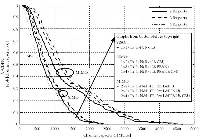
FIGURE 9.1
Channel capacity for the EU transmit power mask.

FIGURE 9.2
Channel capacity for the US transmit power mask.

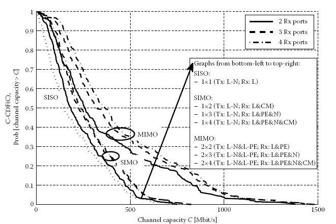
FIGURE 9.3
Channel capacity for the JP transmit power mask.

TABLE 9.1

MIMO Configurations

MIMO Configuration	Tx Ports	Rx Ports
1 × 1	D1 (L-N)	S1 (L)
1 × 2	D1 (L-N)	S1 (L) and S4 (CM)
1 × 3	D1 (L-N)	S1 (L), S2 (N) and S3 (PE)
1 × 4	D1 (L-N)	S1 (L), S2 (N), S3 (PE) and S4 (CM)
2 × 2	D1 (L-N) and D3 (L-PE)	S1 (L) and S3 (PE)
2 × 3	D1 (L-N) and D3 (L-PE)	S1 (L), S2 (N) and S3 (PE)
2 × 4	D1 (L-N) and D3 (L-PE)	S1 (L), S2 (N), S3 (PE) and S4 (CM)

Table 9.2 summarises the median value (50% point) and the 98% point (high coverage point) of the C-CDF shown in the Figures 9.1 through 9.3. The following observations may be drawn from the figures and the table. First, consider the median values:

•  The SIMO configurations with only one transmit port already offer a gain compared to SISO. The channel capacity of the best SIMO scheme, 1 × 4, is increased by 37% (EU mask), 39% (US mask) and 56% (JP mask) compared to SISO. The increasing relative gain starting with the EU mask, followed by the US mask, and ending with the JP mask, is explained considering absolute bitrates. The higher the absolute bitrate, the lower the relative SIMO gain. And vice versa, channels supporting only lower absolute bitrates offer the highest gain relative to SISO. The same tendency is observed for MIMO in the high coverage area. The overall lower bitrates of the US and JP masks compared to the EU mask are derived from the transmit masks: the US mask is 5 dB below the EU mask, while the JP mask does not even allow any transmission above 30 MHz.

•  Using the second transmit port results in full MIMO configurations and provides a significant increase in bitrate compared to SISO, reflected by 71% (EU and US masks) and 72% (JP mask) for the 2 × 2 scheme and 116% (EU and US masks) and 146% (JP mask) for the 2 × 4 MIMO configuration. (The bitrate increase when applying the JP power transmit mask is hypothetical, because the third wire only rarely exists in JP outlets.)

TABLE 9.2

Channel Capacity and Gain Compared to SISO for Different Transmit Power Masks: Median Values and 98% Coverage Point

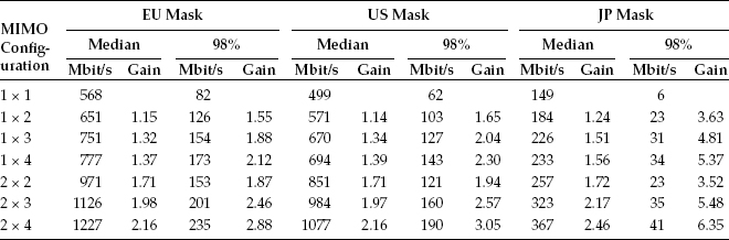
In conclusion, the MIMO channel capacity of the full (2 × 4) MIMO configuration is on average more than double the SISO capacity.

Next, consider the high coverage area (98% point):

•  At the high coverage area, the SIMO configurations already offer a significant gain compared to SISO: factors of 2.12 (EU mask), 2.03 (US mask) and even 5.37 (JP mask) are observed for the 1 × 4 configuration.

•  In contrast to 1 × 4 MIMO, the 2 × 2 configuration provides less gain: 1.87, 1.94 and 3.52 for the EU, US and JP masks, respectively. The second, weaker stream (eigenmode) does not contribute much for low SNR channels. It is more important to collect all the available signal energy at the receiver. This is reflected by the number of receive ports.

•  Combining the use of the maximum number of receive ports and the use of two streams for the 2 × 4 configuration shows the highest gain compared to SISO: 2.88, 3.05 and 6.35 for the EU, US and JP masks, respectively.

The MIMO gain in the high coverage area is even higher compared to the median values. Thus, MIMO especially improves the difficult links with high attenuation and therefore low SNR at the receiver, making MIMO a promising method for meeting ambitious coverage requirements. Note that the presented results are the theoretical channel capacity. The choice of the implemented MIMO scheme and the system parameters for modulation, coding and implementation aspects and limitations influence the achievable throughput in real modem implementations (e. g. a 10 bit analogue-to-digital converter (ADC) might not utilise the full SNR available at the channel).

9.3    MIMO PLC Throughput Analysis

The aim of this section is to verify the MIMO channel capacity gains of the previous section for different MIMO PLC systems. In particular, the OFDM-based MIMO PLC schemes introduced in Chapter 8 are investigated with respect to the achieved bitrate. Adaptive modulation is applied to the SNR after detection (see Section 9.3.1). As for SISO, the SNR after MIMO processing is still very frequency-selective. This makes subcarrier-specific adaptive modulation a good choice for maximising the PLC throughput. The achieved bitrate is analysed in Section 9.3.2 for a large set of MIMO PLC channels.

9.3.1    Adaptive Modulation

The frequency-selective PLC channel leads to high SNR variations for different OFDM subcarriers. To overcome this problem, adaptive modulation is applied. Each subcarrier is bit loaded and modulated according to the corresponding SNR. The higher the SNR, the higher the quadrature amplitude modulation (QAM) constellation. Figure 9.4 shows an example of a typical SISO PLC channel. The SNR, depending on the frequency from 4 to 30 MHz, illustrates the frequency-selective channel. The QAM constellations with modulation order M used here are binary phase-shift keying (BPSK) (M = 2) and the even or square QAM constellations from quadrature phase-shift keying (QPSK) to 4096-QAM (M = 4, 16, 64, 256, 1024, 4096). The number of bits per QAM symbol is log₂(M). The SNR thresholds θ_M for each modulation order M are illustrated by the horizontal lines in Figure 9.4 for each modulation scheme. These thresholds define the assignment of the QAM constellation depending on the SNR of each subcarrier. A subcarrier can also be omitted (notched) if the SNR is too low to carry any information.

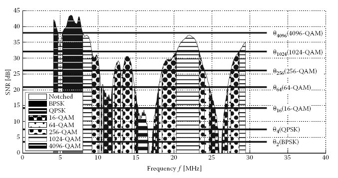
FIGURE 9.4
Adaptive modulation: available SNR depending on the frequency, and application of QAM constellations depending on the available SNR, SISO, transmit power to noise power level ρ = 65 dB.

If Λ(n) is the SNR of subcarrier $n\left(1\le n\le N\right)$, the assignment to modulation order M(n) of subcarrier n depends on the thresholds θ_M of each modulation order M:

$M\left(n\right)=\{\begin{array}{cc}1,& \text{Λ}\left(n\right)<{\text{θ}}_2\left(\text{not}\text{modulated}\right).\\ 2,& {\text{θ}}_2\le \text{Λ}\left(n\right)<{\text{θ}}_4\left(\text{BPSK}\right).\\ 4,& {\text{θ}}_4\le \text{Λ}\left(n\right)<{\text{θ}}_{16}\left(\text{QPSK}\right).\\ 16,& {\text{θ}}_{16}\le \text{Λ}\left(n\right)<{\text{θ}}_{64}\left(16\text{-QAM}\right).\\ 64,& {\text{θ}}_{64}\le \text{Λ}\left(n\right)<{\text{θ}}_{256}\left(64\text{-QAM}\right).\\ 256,& {\text{θ}}_{256}\le \text{Λ}\left(n\right)<{\text{θ}}_{1024}\left(256\text{-QAM}\right).\\ 1024,& {\text{θ}}_{1024}\le \text{Λ}\left(n\right)<{\text{θ}}_{4094}\left(1024\text{-QAM}\right).\\ 4096,& {\text{θ}}_{4096}\le \text{Λ}\left(n\right)\left(4096\text{-QAM}\right).\end{array}$

(9.12)

In Equation 9.12, the modulation order M = 1 indicates that no information is assigned to the subcarrier, that is, log₂(1) = 0 bit is assigned. The choice of the SNR thresholds θ_M influences both the achieved bitrate and the bit error ratio (BER).

The bitrate D is the sum of the bits assigned to each subcarrier divided by the OFDM symbol length T_u:

$D=\frac{{\displaystyle {\sum }_{n=1}^L{\log }_2\left(M\left(n\right)\right)}}{T_u}.$

(9.13)

The BER depends on the SNR Λ and the modulation order M. For an AWGN channel, the BER is given by the tight approximation [19,20]:

$P_b\left(M,\text{Λ}\right)=\{\begin{array}{cc}\frac{1}{2}\cdot \text{erfc}\left(\sqrt{\mathrm{\Lambda }}\right),& M=2,\\ \frac{2}{{\log }_2\left(M\right)}\cdot \left(1-\frac{1}{\sqrt{M}}\right)\cdot \text{erfc}\left(\sqrt{\frac{3\text{Λ}}{2\left(M-1\right)}}\right),& {\log }_2\left(M\right)\text{even}\end{array}$

(9.14)

with $\text{erfc}\left(x\right)=\frac{2}{\sqrt{\text{π}}}{\displaystyle {\int }_x^{\infty }\exp \left(-t^2\right)}dt$ being the complementary error function. Binary reflected Gray bit labelling is assumed for the even constellations (log₂(M) even) in Equation 9.14.

With M(n) the modulation order and Λ(n) the SNR of subcarrier $n\left(1\le n\le N\right)$, the BER of each subcarrier P_b(M(n),Λ(n)) can be calculated according to Equation 9.14. The overall average BER ${\overline{P}}_b$ is given as the average number of bits in error divided by the total number of transmitted bits [20] and can be calculated as

${\overline{P}}_b=\frac{\text{Number}\text{of}\text{errors}}{\text{Number}\text{of}\text{bits}}=\frac{{\displaystyle {\sum }_{n=1}^N{P}_p\left(M\left(n\right),\text{Λ}\left(n\right)\right)\cdot {\log }_2\left(M\left(n\right)\right)}}{{\displaystyle {\sum }_{n=1}^N{\log }_2\left(M\left(n\right)\right)}}.$

(9.15)

Recall that the SNR thresholds θ_M determine the modulation order M(n) of each subcarrier according to Equation 9.12 and thus influence both the bitrate according to Equation 9.13 and the average BER according to Equation 9.14. The design of the SNR thresholds θ_M can be optimised with respect to two different criteria:

•  Minimising the BER for a fixed bitrate

•  Maximising the bitrate for a fixed BER

The second criterion is considered here. A simple algorithm that guarantees a certain target BER $P_b^{\prime }$ with ${\overline{P}}_b\le P_b^{\prime }$ uses fixed SNR thresholds. For a given target BER $P_b^{\prime }$ and modulation order M, Equation 9.14 can be solved for Λ which is then used as SNR threshold θ_M. Figure 9.5 shows the BER depending on the SNR for different modulation orders. The figure also provides the SNR thresholds for a target BER of $P_b^{\prime }$ = 10⁻³. The BER value of 10⁻³ may be sufficient for the raw physical layer since additional forward error correction (FEC) will improve the BER. This algorithm guarantees that the average BER ${\overline{P}}_b$ does not exceed the target BER $P_b^{\prime }$ in every case. Usually, the average BER $\overline{P}$ will be lower than the target BER $P_b^{\prime }$ since many subcarriers have higher SNR than the SNR thresholds.

Schneider et al. [5,8] propose an algorithm which maximises the bitrate D, for a desired target BER $P_b^{\prime }$. The algorithm takes the SNR distribution of the given channel into account, that is, the algorithm adapts the SNR thresholds to the current channel conditions.

The SNR thresholds shown in Figure 9.4 are obtained according to the algorithm described earlier for a target BER of 10⁻³. Note that the SNR thresholds are lower compared to the fixed SNR thresholds shown in Figure 9.5. Thus, the bitrate of the proposed algorithm is higher compared to the algorithm with fixed thresholds.

The MIMO scheme and detection algorithm determine the SNR of the MIMO streams as shown in Chapter 8. Adaptive modulation is applied for each MIMO stream separately. Figure 9.6a shows the block diagram of the adaptive modulation algorithm for MIMO. The SNR thresholds θ_M are calculated according to the SNR of the subcarriers after MIMO detection. These thresholds are used to assign the QAM constellation to each subcarrier. Note that the blocks adaptive QAM pattern and adaptive thresholds in Figure 9.6 require knowledge of the SNR for all subcarriers; thus, these blocks operate in parallel. The calculation of the PA coefficients is based on the SNR and the QAM constellations (see Section 8.3). This results in a dependency between the PA and the adaptive modulation as highlighted in Figure 9.6b. The combination of adaptive modulation and PA has to be calculated iteratively in this case.

FIGURE 9.5
BER depending on SNR for different QAM orders and SNR values required for a target BER of 10⁻³.

9.3.2    Simulation Results

The MIMO-OFDM system described in Chapter 8 forms the basis of the system simulations. 1296 subcarriers are used in the frequency range from 4 to 30 MHz. Each subcarrier is adaptively modulated, according to the adaptive modulation algorithm described in Section 9.3.1. The target average BER of the uncoded system is adjusted to 10⁻³. An additional FEC might easily reduce this BER. The bitrate is obtained as the sum of the number of bits assigned to all subcarriers divided by the OFDM symbol length. This bitrate describes the raw physical layer bitrate without considering the guard interval length, training data or FEC overhead. The basic system parameters are summarised in Table 9.3.

The noise is modelled by AWGN with zero mean, and it is assumed that the noise is uncorrelated and that the noise power is the same for all receive ports. The transmit power to noise power level is assumed to be ρ = 65 dB. This value corresponds to a transmit PSD of −55 dBm/Hz (see Chapter 6) and an average noise PSD of −120 dBm/Hz (this corresponds to the 90% point of CDF of the noise according to Chapter 5). Impulsive noise is not considered. The focus is on the comparison between MIMO and SISO schemes. It is expected that impulsive noise will influence all receive ports in a similar way. Thus, mitigation techniques known from SISO systems can be applied [21,22]. The measured MIMO PLC channels obtained during the European measurement campaign (ETSI STF410, see Chapter 5) are used in the system simulations. In the case of MIMO, the two feeding ports D1 and D3 (i.e. L-N and L-PE, see Chapter 1) and all four receive ports (S1, S2, S3 and S4) are used; in the case of SISO, the D1 (L-N) port is used at the transmitter and the S1 port (L) at the receiver. It was observed that using the S2 (N) at the receiver yields the same performance as using the S1 port. The corresponding SNR is calculated based on the channel matrix of each subcarrier (channel estimation is assumed to be perfect), depending on the MIMO scheme as shown in Chapter 8. Then, the derived SNR is used with the adaptive modulation algorithm to determine the subcarrier’s constellations. Adaptive modulation is applied to each of the MIMO schemes in this section.

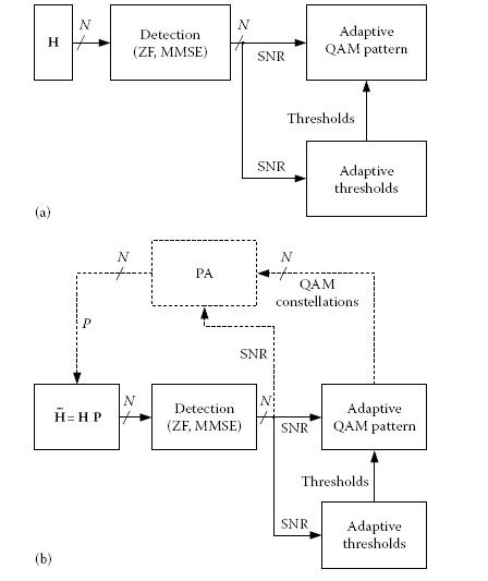
FIGURE 9.6
Block diagram of the adaptive modulation algorithm, without PA (a) and with PA (b).

TABLE 9.3

Basic System Parameters

FFT points	2048
Nyquist frequency (MHz)	40
Frequency band (MHz)	4–30
Number of active subcarriers (4–30 MHz)	1296
Carrier spacing (kHz)	19.53
Symbol length (μrs)	51.2
Modulation (per subcarrier)	BPSK, QPSK, 16-, 64-, 256-, 1024-, 4096-QAM
Uncoded target BER	10−3

Figure 9.7 compares the C-CDF of the bitrate at ρ = 44 dB for different MIMO schemes, namely, SISO, the Alamouti scheme and spatial multiplexing (SMX) with different detection algorithms (see Chapter 8) and BF. The measured MIMO PLC channels form the basis of the comparison. No PA is applied here. SISO is expected to offer the lowest bitrate. However, SMX with zero-forcing (ZF) detection performs about the same or even worse, compared to SISO for most channels and bitrates up to about 40 Mbit/s. The high correlation of the power line channels results in high values of the detection matrix entries, leading to an amplification of the noise (refer also to Section 8.6). This effect is mitigated using more advanced detection algorithms. The bitrate is increased, as seen in Figure 9.7 for minimum mean squared error (MMSE), successive interference cancellation (SIC)-ZF and SIC-MMSE. Ordered SIC (OSIC) receivers are not shown in Figure 9.7, because their performance improvement compared to SIC is only marginal. Eigenbeamforming (EBF) achieves the highest bitrate. The Alamouti scheme performs almost as well as EBF, especially for low bitrates or the high coverage point. The bitrate gain of MIMO compared to SISO is highest for the low bitrate region in Figure 9.7, that is, for channels with high attenuation.

Figure 9.8 is similar to Figure 9.7 with a higher transmit signal to noise power level of ρ = 65 dB. Here, SMX with ZF detection overrides SISO in contrast to Figure 9.7.

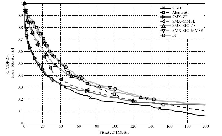
FIGURE 9.7
C-CDF of the bitrate for different MIMO schemes, ρ = 44 dB, no PA, N_T = 2, N_R = 4.

FIGURE 9.8
C-CDF of the bitrate for different MIMO schemes, ρ = 65 dB, no PA,N_T = 2, N_R = 4.

The gain of MMSE versus ZF becomes smaller compared to the lower transmit to noise power level in Figure 9.7. The SIC receivers reach the performance of EBF. However, it has to be kept in mind that no PA and no error propagation of the SIC receiver are considered here. The Alamouti scheme performs well for high values of the C-CDF, that is, for channels with low bitrate due to high attenuation and correlation. However, due to the transmission of replicas, no multiplexing gain is achieved for channels with high bitrate (as can be seen by the low values of the C-CDF in Figure 9.8 where the line of the Alamouti scheme reaches the SISO’s line).

Figure 9.9 compares the PA for SMX and EBF for ρ = 44 dB and ρ = 65 dB. There is only a marginal performance improvement of mercury water filling (MWF) compared to the simplified PA (as introduced in Chapter 8). The gain of PA is most visible for low ρ. As explained also by the SNR results in Chapter 8 (see Figure 8.14), EBF benefits most from PA. The PA’s gain of SMX (SMX-ZF) is relatively small. This is observed for all different receivers for SMX.

Figure 9.10 is similar to Figure 9.7. However, it includes PA. Additionally, one-stream BF is shown where the total power is assigned to the first stream. Figure 9.10a shows the complete coverage range, Figure 9.10b shows the median coverage point and Figure 9.10c shows the high coverage point. Most carriers of the EBF’s second stream turn out to carry no information for highly attenuated channels. The shift of the second stream’s power to the first stream of EBF results in 3 dB higher SNR of the first stream if none of the carriers of the second stream are carrying any information. Obviously, the performance of one-stream BF is close to two-stream BF because as only a few carriers of the second stream contribute to the bitrate. The superior performance of BF over the Alamouti scheme is more visible compared to no PA in Figure 9.7. Please note that PA cannot be used for the Alamouti scheme since each symbol is transmitted via each transmit port.

FIGURE 9.9
C-CDF of the bitrate for spatial multiplexing (SMX-ZF), beamforming (BF) and different PA schemes: no PA, simplified PA and MWF, ρ = 44 dB and ρ = 65 dB, N_T = 2, N_R = 4.

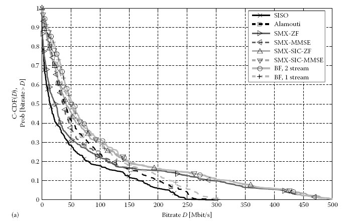
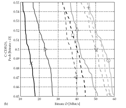
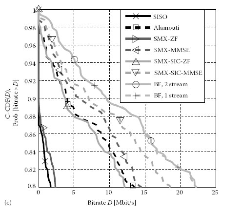
FIGURE 9.10
(a) C-CDF of the bitrate for different MIMO schemes with PA, ρ = 44 dB, N_T = 2, N_R = 4. (b,c) C-CDF of the bitrate for different MIMO schemes with PA, ρ = 44 dB, N_T = 2, N_R = 4.

TABLE 9.4

Mean Values of the Bitrates for Different MIMO and Power Allocation Schemes, 2 × 4 MIMO Configuration

Table 9.4 summarises the mean values of the bitrates for the different MIMO schemes. The two transmit to noise power levels of ρ = 44 dB and 65 dB are considered. The gain of a MIMO scheme is defined as the ratio of the MIMO bitrate to the SISO bitrate.

9.4    Conclusions

This chapter analysed the theoretical MIMO channel capacity based on an extensive measurement set of MIMO PLC channels obtained during the ETSI measurement campaign of STF410. The channel capacity was computed under different regulatory constraints, that is, different transmit power masks. Not only were the measured MIMO CTF taken into account but also the measured noise statistics, which incorporate the spatial correlation of the noise. The MIMO channel capacity is, on average, doubled compared to SISO. In particular, highly attenuated channels benefit most from the application of MIMO which makes MIMO a promising method for improving PLC coverage.

In a next step, the gain of throughput was verified for different MIMO PLC systems. Adaptive modulation was applied to the SNR after MIMO detection of the MIMO PLC schemes introduced in Chapter 8, and the achieved bitrate was analysed. Similar conclusions as for the SNR analysis in Chapter 8 can be drawn for the throughput analysis. Generally, there is a significant increase of bitrate for all MIMO schemes compared to SISO transmission. This confirms the channel capacity gain found in the first part of this chapter. The Alamouti scheme improves the bitrate compared to SISO and showed good performance for highly attenuated channels. However, no multiplexing gain is achieved because of the transmission of replicas of each symbol. Adaptive modulation already adapts to the frequency-selective channel, making the property of the Alamouti scheme to combat fading counterproductive. SMX increases the bitrate compared to the Alamouti scheme for low attenuated channels. Care has to be taken with respect to which MIMO detection algorithm is used. ZF detection fails for a high correlation of the channel, and more complex detection algorithms (like MMSE and SIC) are suggested to increase the performance. The earlier MIMO schemes are open-loop MIMO schemes which require no channel state information at the transmitter. An additional performance gain is achieved by closed-loop MIMO schemes like BF which use channel state information at the transmitter. BF offers the highest bitrate in all scenarios and comes closest to the channel capacity by adapting the transmission to the eigenmodes of the channel. The full spatial diversity gain is achieved for highly attenuated channels and maximum bitrate gain is achieved for channels with low attenuation.

BF requires knowledge about the channel state information at the transmitter. Usually, only the receiver has channel state information. Thus, information about the precoding matrix has to be fed back from the receiver to the transmitter. The application of adaptive modulation already requires feedback about the constellation maps from the receiver. This feedback path might also be used to return the BF information to the transmitter. The feedback rate can be kept low because the in-home PLC channel is less time varying compared to, for example, a mobile channel. Schneider et al. [5,8] investigated the amount of feedback overhead needed to feed back the information about the precoding matrices and showed that the required feedback for the precoding matrices lies in the same order of magnitude as the feedback required for adaptive modulation. For these reasons, a BF-based MIMO-OFDM system with adaptive modulation is a well-suited MIMO system for PLC. The adoption of MIMO and precoded SMX or BF to the latest PLC specifications is discussed in detail in Chapter 12 for G.hn/G.9963 and in Chapter 14 for HomePlug AV2. A study of a MIMO PLC hardware implementation with BF can be found in Chapter 24.

References

1.  A. Paulraj, D. Gore, R. Nabar and H. Bolcskei, An overview of MIMO communications – A key to gigabit wireless, Proceedings of the IEEE, 92(2), 198–218, February 2004.

2.  L. Schumacher, L. T. Berger and J. Ramiro Moreno, Recent advances in propagation characterisation and multiple antenna processing in the 3 GPP framework, in XXVIth URSI General Assembly, Maastricht, the Netherlands, August 2002, session C2. [Online] Available: http://www.ursi.org/Proceedings/ProcGA02/papers/p0563.pdf.

3.  A. Goldsmith, S. Jafar, N. Jindal and S. Vishwanath, Capacity limits of MIMO channels, Selected Areas in Communications, IEEE Journal on, 21(5), 684–702, 2003.

4.  L. Stadelmeier, D. Schneider, D. Schill, A. Schwager and J. Speidel, MIMO for inhome power line communications, in International Conference on Source and Channel Coding (SCC), ITG Fachberichte, Ulm, Germany, 2008.

5.  D. Schneider, J. Speidel, L. Stadelmeier and D. Schill, Precoded spatial multiplexing MIMO for inhome power line communications, in Global Telecommunications Conference, IEEE GLOBECOM, New Orleans, LA, 2008.

6.  R. Hashmat, P. Pagani, A. Zeddam and T. Chonavel, MIMO communications for inhome PLC networks: Measurements and results up to 100 MHz, in International Symposium on Power Line Communications and Its Applications, Rio de Janeiro, Brazil, 2010, pp. 120–124.

7.   A. Schwager, Powerline communications: Significant technologies to become ready for integration, Dr.-Ing. dissertation, Universität Duisburg-Essen, Germany, May 2010.

8.  D. Schneider, Inhome power line communications using multiple input multiple output principles, Dr.-Ing. dissertation, Verlag Dr. Hut, Germany, January 2012.

9.  C. Shannon, Communication in the presence of noise, Proceedings of the IRE, 37(1), 10–21, 1949.

10.  A. Paulraj, R. Nabar and D. Gore, Introduction to Space–Time Wireless Communications. Cambridge University Press, New York, 2003.

11.  R. Hashmat, P. Pagani and T. Chonavel, MIMO capacity of inhome PLC links up to 100 MHz, in Workshop on Power Line Communications, Udine, Italy, 2009.

12.  A. Canova, N. Benvenuto and P. Bisaglia, Receivers for MIMO-PLC channels: Throughput comparison, in International Symposium on Power Line Communications and Its Applications, Rio de Janeiro, Brazil, 2010, pp. 114–119.

13.  D. Rende, A. Nayagam, K. Afkhamie, L. Yonge, R. Riva, D. Veronesi, F. Osnato and P. Bisaglia, Noise correlation and its effect on capacity of inhome MIMO power line channels, in International Symposium on Power Line Communications and Its Applications, Udine, Italy, 2011, pp. 60–65.

14.  F. Versolatto and A. Tonello, A MIMO PLC random channel generator and capacity analysis, in International Symposium on Power Line Communications and Its Applications, Udine, Italy, 2011, pp. 66–71.

15.  D. Schneider, A. Schwager, W. Bäschlin and P. Pagani, European MIMO PLC field measurements: Channel analysis, in International Symposium on Power Line Communications and Its Applications, Beijing, China, 2012, pp. 304–309.

16.  ETSI, TR 101 562-1 v1.3.1, Powerline telecommunications (PLT), MIMO PLT, part 1: Measurement methods of MIMO PLT, Technical Report, 2012.

17.  ETSI, TR 101 562-2 v1.2.1, Powerline telecommunications (PLT), MIMO PLT, part 2: Setup and statistical results of MIMO PLT EMI measurements, Technical Report, 2012.

18.  ETSI, TR 101 562-3 v1.1.1, Powerline telecommunications (PLT), MIMO PLT, part 3: Setup and statistical results of MIMO PLT channel and noise measurements, Technical Report, 2012.

19.  S. T. Chung and A. Goldsmith, Degrees of freedom in adaptive modulation: A unified view, IEEE Transactions on Communications, 49(9), 1561–1571, September 2001.

20.  J. Proakis, Digital Communications, 4th ed. McGraw-Hill Book Company, New York, 2001.

21.  E. Biglieri, Coding and modulation for a horrible channel, IEEE Communications Magazine, 41(5), 92–98, 2003.

22.  D. Fertonani and G. Colavolpe, On reliable communications over channels impaired by bursty impulse noise, IEEE Transactions on Communications, 57(7), 2024–2030, 2009.