5

Broadband In-Home Statistics and Stochastic Modelling

Andreas Schwager, Pascal Pagani, Daniel M. Schneider, Rehan Hashmat and Thierry Chonavel

CONTENTS

5.1    Motivation

5.2    Statistical Evaluation of Results

5.2.1    CTF and Attenuation

5.2.2    Reflection (S₁₁)

5.2.3    Noise

5.2.3.1    Frequency Domain Results

5.2.3.2    Time Domain Results

5.2.4    Singular Values and Spatial Correlation

5.3    Statistical Modelling of the PLC MIMO Channel Based on Experimental Data

5.3.1    MIMO CTF Modelling

5.3.1.1    Median Channel Gain Modelling

5.3.1.2    Frequency Domain Path Loss Modelling

5.3.1.3    Multi-Path Model for the SISO Line-Neutral (D1) to Line (S1) Path

5.3 1.4    Extension of the Multi-Path Model to the MIMO Channel Matrix

5.3.1.5    Evaluation of the Channel Model

5.3.2    Multiple-Output Noise Modelling

5.3.2.1    Multivariate Time Series

5.3.2.2    Figures of Merit for Model Validation

5.3.2.3    Vector Autoregressive Model

5.3.2.4    Order Selection and Extraction of the VAR Model

5.3.2.5    Results and Model Validation

5.4    Conclusion

Acknowledgements

References

5.1    Motivation

PLC systems available today use only one transmission path between two outlets. It is the differential-mode (DM) channel between the phase (or live) and neutral contact of the mains. These systems are called single input single output (SISO). In contrast, multiple-input multiple-output (MIMO) PLC systems make use of the third wire, protective earth (PE), which provides several transmission combinations for feeding and receiving signals into and from the low-voltage distribution network (LVDN). Various research publications, for example, [1,2,3] describe up to eight transmission paths that might be used simultaneously in the home.

Channel measurements, as described in this publication, are verified by the European Telecommunications Standards Institute (ETSI).A Special Task Force was set up [4] in 2010 to record MIMO channel, noise and electromagnetic interference (EMI) properties in many European countries.

As MIMO PLC modems also utilise the protective earth, they are able to alternately feed from live to neutral (L-N), live to protective earth (L-PE) and neutral to protective earth (N-PE). The protective earth may be grounded inside (e.g. at the foundations) or outside (at the transformer station) the building and provides low impedance for the 50 Hz AC power. However, high-frequency signal measurements show the PE wire to be a rather excellent communication path which by no means represents a ground. This is due to the inductivity of the long PE wires.

This chapter provides a statistical evaluation of these properties plus the spatial correlation of the MIMO paths. In addition, the noise received in a MIMO PLC system is analysed. Information on the presence of the protective earth wire, on measurement methods, and on MIMO topologies and corresponding coupling devices are described in detail in Chapter 1. Finally, this chapter presents new models of the MIMO channel transfer function (CTF) and multiple-output noise, based on the observed statistics.

5.2    Statistical Evaluation of Results

5.2.1    CTF and Attenuation

S21 of MIMO PLC channels was measured in 36 buildings. Records of 4684 sweeps in total were collected using a network analyser (NWA). Each sweep recorded the attenuation of 1601 frequency values which resulted in 7,499,084 measures for the statistical analysis later.

Figure 5.1 depicts an example of individual sweeps of all MIMO paths between two outlets. There are 12 sweeps in total transmitted at the delta ports D1, D2 and D3 and received at the star ports S1, S2, S3 and the CM port S4. The ports described here and the PLC coupler used for the measurements are described in Chapter 1. The black area in Figure 5.1 shows the distance from the minimum attenuation of all sweeps to the maximum values. Additionally, three individual records are given. The area between the paths is 15 dB up to 35 dB wide depending on the frequency. An increasing attenuation towards the higher frequencies is visible. Chapter 9 shows that the more deviation a link provides between the individual paths, the more gain will be achieved when utilising MIMO technology. Frequency-modulated (FM) radio reception was excellent in the location where Figure 5.1 was recorded. Some ingress of FM radio stations onto the NWA data is also visible in the graphs. Electromagnetic compatibility between PLC and FM radio reception will be discussed in Chapter 7.

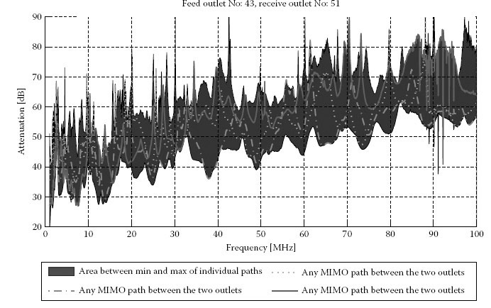
FIGURE 5.1
All MIMO paths between two outlets.

[Figure 5.2 represents the cumulative probability of measuring such as attenuation. Usually, a stretched S-style line from the bottom-left to top-right corner is depicted in the graph. These figures may be read in the following way:

•  Top-right corner, 100% or ‘always’ point: The maximum recorded value in Figure 5.2 is 100 dB attenuation.

•  80% point at light grey line (Δ marker) in Figure 5.2: 80% of all measured values provide less attenuation than 66 dB when feeding style D1 (SISO feeding between live and neutral) is selected.

•  Median or 50% point: Every second measured value provides higher or lesser attenuation than ∼53 dB in Figure 5.2.

•  Lower left corner, the 0% or ‘never’ point: The attenuation was never smaller than 5 dB (minimum point outside Figure 5.2).

All attenuation measurements – independent of location, country or frequency – are separated into individual feeding possibilities: D1, D2 and D3 on delta coupler and T1 and T2 at T-style coupler. Their statistical distribution is visualised in Figure 5.2. A zoom into the high attenuated records (lower-right figure in Figure 5.2) shows that the T-style coupler provides better PLC coverage. They are less attenuated than other feeding styles. The two wires used for traditional PLC modems (live–neutral, D1) show the worst coverage in this case. This is probably caused by multiple consumers connected to live and neutral inside homes.

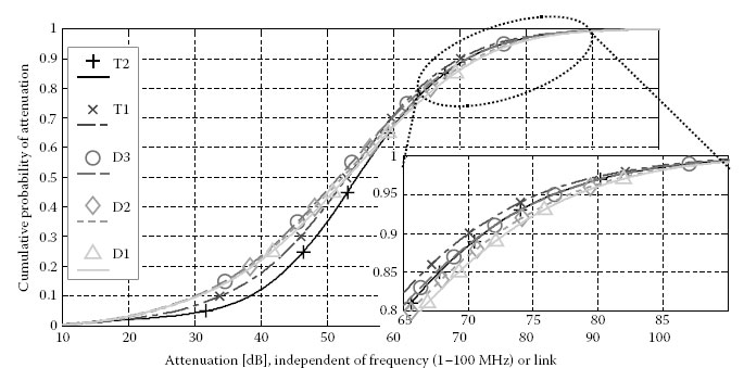
FIGURE 5.2
Statistical distribution of attenuation for all feeding styles.

NOTES: The unused ports at the coupler were terminated with 50 Ω in these measurements. The classical SISO style modems operate by sending and receiving signals symmetrically via P and N. Unused feeding combinations in SISO are either open or unterminated. Termination of unused ports, when identical energy is fed into the couplers, theoretically consumes 1.96 dB of signal energy from mains wires compared to an unterminated coupler where no loss takes place.

Results for the possibility of receiving – identical analytical process as applied for the transmission possibilities – are displayed in Figure 5.3. In the lower right corner is a close up of the high attenuated values. These statistics are derived from identical measurements already presented in Figure 5.2 but sorted by individual receiving styles. Of the receiving possibilities displayed, CM reception on the coupler’s port S4 (◊) provides the best coverage (less attenuation at high attenuated channels).

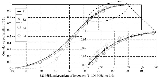
FIGURE 5.3
Cumulative probability of attenuation (S21) of all receiving styles.

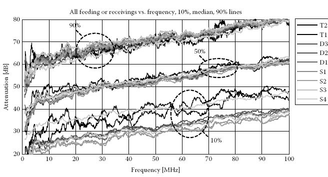
FIGURE 5.4
Attenuation (S21) depending on frequency.

NOTES: The coupler itself is considered to be part of the channel in these statistics. ETSI TR 101562 in clause 7.1.6 [5] shows that CM reception with the STF 410 coupler increases attenuation by 3–4 dB compared to reception on S1, S2 or S3. If someone is interested in the channel attenuation without the influence of the STF 410 coupler, the coupler verification values from ETSI TR 101562 [5,6,7]^* might be considered causing the S4 (CM) line to move to lower attenuated records. The gap between the CM line and the others becomes larger at high attenuated values.

The 10% values, median values and 90% values at each frequency, for all feeding and receiving styles, are shown in Figure 5.4. A bunch of curves for each feeding and receiving port is shown three times in Figure 5.4. The top bunch increasing over frequency from 60 to 80 dB represents the 90% values of all attenuations over the frequency. These are the high attenuated channels out of the top-right corners of Figures 5.2 and 5.3. The median values out of all sweeps are shown by the middle bunch of Figure 5.4. The 10% values have a higher standard variation and are the lower bunch in Figure 5.4. A constant trend from 5 to 100 MHz can be observed, where higher frequencies are more attenuated than lower frequencies. This trend is independent of the feeding or receiving port. This slope is 0.2 dB/MHz. This frequency trend is valid at high as well as at low attenuated channels.

Figure 5.5 shows that the CM path (received on port S4 and marked with ◊) provides less attenuation in higher attenuated channels. Figure 5.5 shows a graph of the top 90% of attenuated values depending on frequency. The phenomenon of the CM having less attenuation than the DM signals or single-ended lines (S1, S2 or S3) exists at all frequencies.

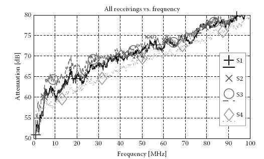
FIGURE 5.5
Statistical 90% value of attenuation at higher attenuated records. Depending on frequency and receiving port.

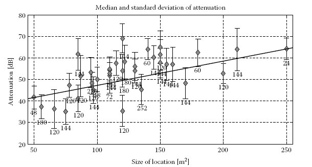
FIGURE 5.6
Size of location, median attenuation, standard deviation and number of sweeps.

It is interesting to compare the median values and the standard deviation of attenuation at each location. The number of sweeps at each location gives an indication of the size and maturity of the statistics.Figure 5.6 shows median attenuation using the diamonds; the standard deviation is indicated by the error bars. The number of sweeps is listed below each error bar.

Figure 5.6 displays the relationship between the size of the location under measurement and the attenuation between two outlets. Assuming a linear relationship between these two parameters, a fitting line can be drafted into Figure 5.6. The formula of this line is

$\text{Attenuation}\left(\text{dB}\right)=0.11\text{dB}/{\text{m}}^2*\text{size}\left({\text{m}}^2\right)+36.07\text{dB}\text{.}$

Figure 5.7 shows the median attenuation of all attenuation records of each country. Highest attenuation is found in Germany. This is caused by the three-phase installations in German homes. Additionally, the error bars give the standard deviation. It is interesting to see that the standard deviation is almost identical in all countries. The results of an individual record at an outlet vary heavily to the other outlet or location. However, comparing a statistical mass of data between two locations shows always identical results. The numbers given on each bar indicate the number of sweeps recorded in this country.

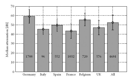
FIGURE 5.7
Median attenuation of each country.

The mains installation in the United Kingdom and the Commonwealth of Nations uses a ring wire on each housing level. The outlets are daisy chained along the ring. As a result each outlet is connected to two sets of wires, each going in a different direction in the room. Electrical installations in the rest of the world follow a combination of star (at the fuse cabinet) and tree style (branches into rooms, outlets, light switches, etc.). Even the ring-wire installations used in the United Kingdom do not show any major difference results here.

5.2.2    Reflection (S₁₁).

Reflection measurements were conducted in 33 locations in Belgium, France, Italy, Germany, Spain and the United Kingdom. In total, 661 frequency sweeps have been recorded with 1601 points in each frequency domain. This results in a statistical compilation of 1,058,261 values.

Figure 5.8 presents a sweep recording the reflection parameter at the star coupler. The three single-ended ports S1 (◊), S2 (o) and S3 (×) show above 10 MHz a very similar reflection characteristic compared to the attenuation measurements shown earlier. The CM termination (S4, +) is different to the others and provides less fading over the frequency.

Figure 5.9 shows an overview of the probability of measuring a reflection parameter of all S₁₁ measurements. Indoor power line networks show weak impedance conditions. Due to the high variations of S₁₁ parameters, it is difficult to implement impedance matching couplers. Time-, frequency-and location-dependent characteristics influence the coupler’s feeding or receiving properties. A S₁₁ parameter of zero or negative infinite in the logarithm representation shows optimal termination, nothing is reflected. If this parameter equals 1 in linear representation or 0 dB, the full wave is reflected. If the S₁₁ parameter is worse than −6 dB (−6 dB < S₁₁ < 0 dB), more than half of the fed signals are reflected back to the coupler at the connected outlet. This is the case for >60% of S₁₁ measurements using the delta-or T-style coupler. Star-style ports offer better termination than the others; T-style ports are the worst.

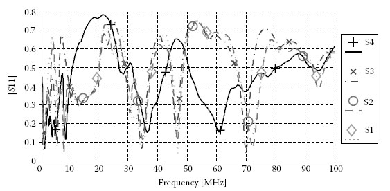
FIGURE 5.8
S₁₁ at the star-style coupler at a typical outlet.

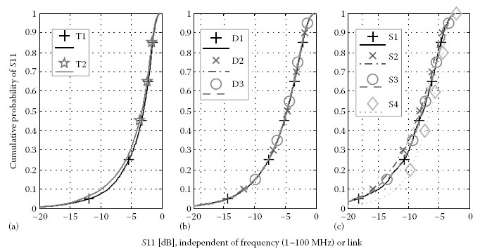
FIGURE 5.9
CDF of magnitude of S₁₁ from T-style (a), delta-style (b) and star-style (c). Independent of location or frequency.

The impedances of the delta ports D1 (o), D2 (×) and D3 (+) at a typical outlet are shown per frequency in Figure 5.10. It is interesting to see the variance of the impedance values in between the individual ports to be small. This phenomenon was also found at the single-ended star ports in Figure 5.8. Obviously, if a MIMO PLC coupler should become impedance matched to the mains, all MIMO paths could be matched identically.

The ring-wire mains installation in the United Kingdom might provide half the impedance of a continental outlet, because the outlet is connected to two sets of wires. Table 5.1 compares the median impedances of UK installations with all measurements recorded on the European continent. As expected, the UK installations show lower impedance but not half the value than found on the continent.

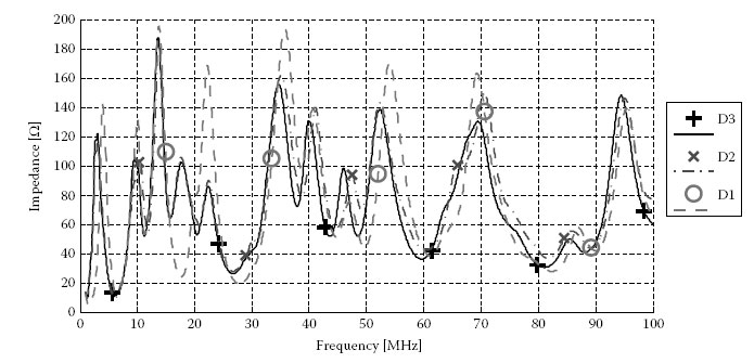
FIGURE 5.10
Impedance Z (delta ports) of a typical outlet.

TABLE 5.1

Median Impedance for each Feeding/Receiving Style

Feeding/Receiving Style	Impedance in Ω, All Locations	Impedance in Ω, All Locations Except United Kingdom	Impedance in Ω, Locations in United Kingdom Only
D1	86.04	86.86	77.14
D2	87.41	88.27	78.31
D3	88.94	89.73	81.96

5.2.3    Noise

Experimental measurements of the MIMO PLC noise were conducted in 31 different dwelling units in five European countries, including Belgium, France, Germany, Spain and the United Kingdom. Measurements were taken in flats and houses of different sizes. On average, four electrical plugs were considered in each location. Considering that the measurement process included four different signals (live, protective earth, neutral and common-mode), and that each signal was recorded using four different filters, the statistical set was constituted of 1928 records measured in the time domain over a duration of 20 ms each.

5.2.3.1    Frequency Domain Results

The first analysis of the collected noise is conducted in the frequency domain up to a maximum frequency of 100 MHz. For this purpose, the power spectral density (PSD) of the recorded noise was estimated using the method of Welch [8]. The final resolution bandwidth (ResBw) of the frequency domain data is 122 kHz, which is comparable to the resolutions commonly used in EMI testing. The ResBw of 122 kHz = 50.9 dB (Hz) was subtracted from the noise records to visualise the noise PSD in Figures 5.11 through 5.16.

First statistical results are depicted in Figure 5.11, where different percentiles of the noise PSD recorded during the experiment over the full frequency band (Band 1) are shown. The considered data set includes all measurements, regardless of the location or the receiver (Rx) port. For each frequency, the graph represents the 1% and 25% percentiles, the median value and the 75% and 99% percentiles. The observed PSD lies within minimum values around −160 dBm/Hz and maximum values around −80 dBm/Hz. The presence of short wave (SW) broadcast frequencies is clearly noticeable at 6, 7.3, 9.5, 12, 13.5, 15.5, 17.5 and 21 MHz (metre bands of 49, 41, 31, 25, 22, 19, 16 and 13 m, respectively). At the highest frequencies above 87 MHz, strong noise peaks reveal the presence of broadcast FM signals.

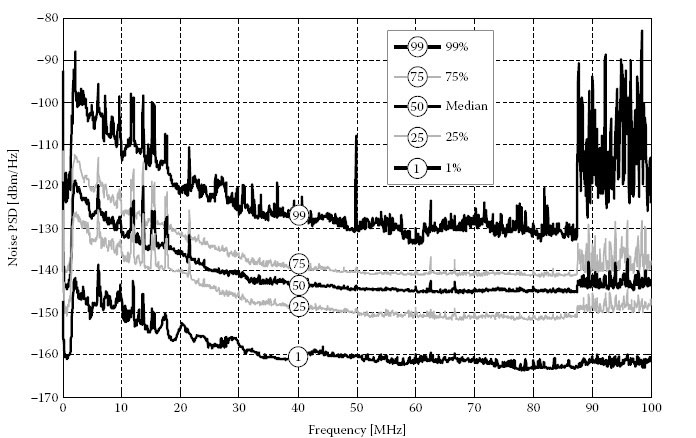
FIGURE 5.11
Statistics of the noise PSD measured on Band 1: 1%, 25%, median, 75% and 99%.

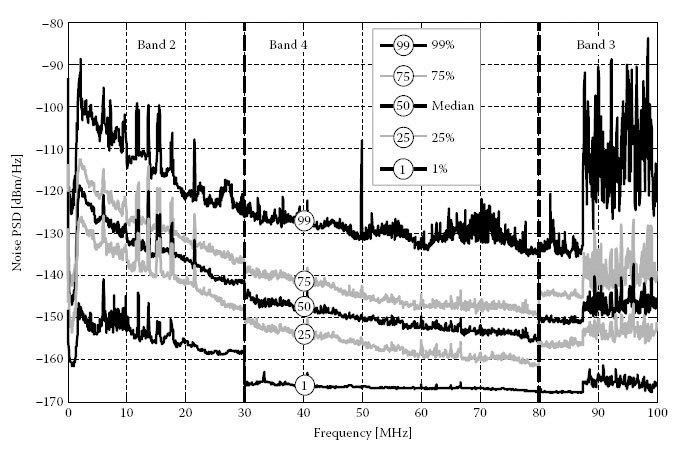
FIGURE 5.12
Statistics of the noise PSD measured on the combined band: 1%, 25%, median, 75% and 99%.

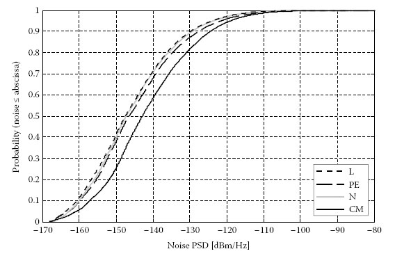
FIGURE 5.13
Statistics of the noise PSD for different reception methods.

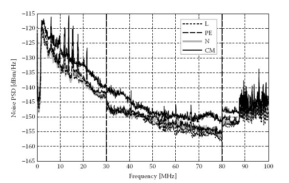
FIGURE 5.14
Median noise PSD measured on the combined band for different reception methods.

In order to be able to observe low noise levels, one needs to make sure that the signal is not contaminated by quantisation effects due to the digital sampling oscilloscope (DSO) limitations. To avoid this problem, noise was also recorded using filters over narrower bands. In the experimental set-up, Band 2 rejected FM signals, Band 3 rejected SW signals and Band 4 rejected both. From these measurements, a combined band was defined by aggregating results from Band 2 over the (0–30 MHz) range, Band 4 over the (30–80 MHz) range and Band 3 over the (80–100 MHz) range.

Figure 5.12 reproduces similar results as in Figure 5.11, based on records from the combined band. Using the combined band mainly improves the sensitivity for the lowest noise values. Considering the 1% percentile, lowest values now reduce to −168 dBm/Hz in the (30–87 MHz) range.

It is now interesting to observe the influence of the reception method on the level of the recorded noise.Figure 5.13 presents the cumulative distribution function (CDF) of the noise PSD for each of the L wire, PE wire, N wire and CM signal. A first observation is that the CM signal is subject to stronger noise than the signals transmitted over the L, PE or N wire. This difference of 5 dB can be explained by the higher sensitivity of the CM signal to interference from external sources, such as radio broadcasting. The L, PE and N ports present similar noise statistics. However, when considering large noise records (5% percentile), one can observe that the PE port is more sensitive to noise by ~2 dB than the N or L ports. Similarly, for low noise records (95% percentile), the L port is less sensitive to noise by ~1 dB than the N or PE ports.

Figure 5.14 presents the median value of the noise PSD measured on the combined band for different reception methods. This frequency domain observation confirms that the CM noise is stronger than the noise collected over each of the L, PE and N wires separately. This difference is particularly noticeable in the frequency range from 1 to 45 MHz. This leads to the assumption that the ingress of noise signals to the mains grid is responsible for the background noise and not conducted noise sources. Another interpretation of this phenomenon is that conducted noise sources mainly generate CM noise instead of DM noise. On the statistical median, the noise observed on the L, PE and N ports appears to take similar values over the whole combined band.

This noise measurement campaign performed in 35 locations in different European countries was the occasion to observe the possible relation between the level of the noise PSD and the size of the location. Without further knowledge, one could assume that larger houses with a larger number of connected electrical appliances would lead to higher observed noise values. Figure 5.15 presents statistics of the recorded noise PSD across the location size. The location size ranges from 50 to 200 m², and noise statistics include the 1% and 25% percentiles, the median and the 75% and 99% percentiles. Statistically, it can be expected that larger homes have more electrical appliances installed. However, one can clearly observe that there is no correlation between the surface of the house and the statistics of the noise PSD level. Using other words, the noise accumulation is independent of the location’s size. One can conclude that the PLC modems will be mostly affected by interferers in their close vicinity or by external broadcast signals. Distant electromagnetic interferers on the same electrical network do not seem to have a noticeable impact on the received noise.

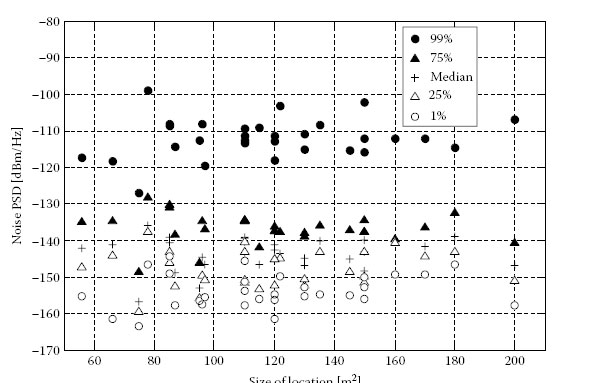
FIGURE 5.15
Influence of the size of the location on the noise statistics.

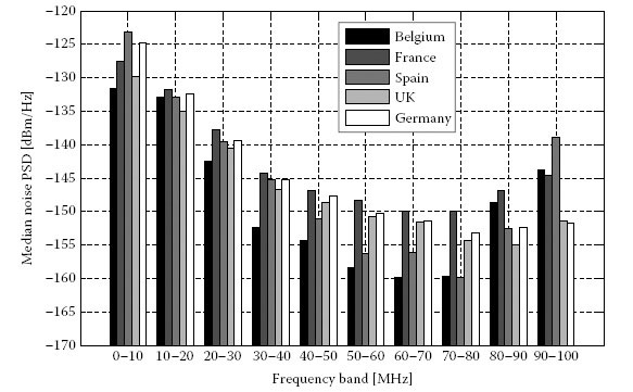
FIGURE 5.16
Median of the noise PSD received over frequency bands of 10 MHz each, separated by country.

Finally, the analysis compares the level of noise received in different countries.Figure 5.16 presents the median value of the noise PSD collected over 10 frequency bands of 10 MHz each, for each of the following countries: Belgium, France, Spain, United Kingdom and Germany. The aggregated data has been collected by considering measurements over the combined band. The level of recorded noise is comparable in Germany, France and United Kingdom, except for frequencies above 70 MHz, where France presents larger values. In Spain, measurements below 10 MHz and above 90 MHz led to the highest noise records, but in the range (40–80 MHz), the values found for this country are among the lowest ones. From measurements taken in Belgium, it can be concluded that the noise level is lower than for the other countries for frequencies below 80 MHz. Nevertheless, in the FM band, strong interference can be observed in Belgian records.

5.2.3.2    Time Domain Results

In the following, the characteristics of the noise are analysed in the time domain. Out of the 1928 records of 20 ms duration each, four typical structures could be identified:

1.  Stationary noise: Most of the records present a flat temporal structure, without noticeable fluctuation. An example of such record is given in Figure 5.17, which is representative of approximately two-thirds of our observations.

2.  Periodical 50 Hz synchronous noise: In some records, a clear periodical structure with a period of 10 ms is observable. This is the case in the example given in Figure 5.18. The period of such a noise structure corresponds to the half of the period of the 50 Hz mains. Such impulsive noise can be generated by, for example, switched mode power supplies or light dimmers. Such structure occurred between 10% and 15% of our observations.

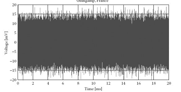
FIGURE 5.17
20 ms noise sample recorded in the time domain, stationary noise.

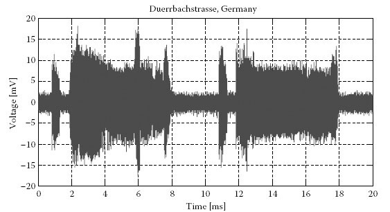
FIGURE 5.18
20 ms noise sample recorded in the time domain, periodical 50 Hz synchronous structure.

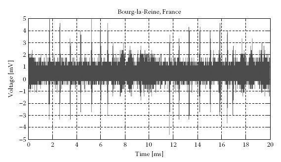
FIGURE 5.19
20 ms noise sample recorded in the time domain, periodical asynchronous structure.

3.  Periodical asynchronous structure: Other records showed a typical periodical structure, but without being synchronised with the 50 Hz mains.Figure 5.19 presents such a periodical, asynchronous noise, with impulses reproduced at a rate of 1.3 kHz. This type of noise could be observed in 10% to 15% of our records, and can be generated by, for example, electronic devices or compact fluorescent lamps.

4.  Strong impulsive structure: In the database, some noise records presented larger voltage values and an impulsive structure, like the sample depicted in Figure 5.20. This strong impulsive structure is observed in 10%–15% of the cases.

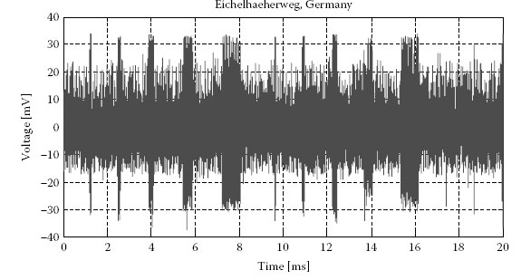
FIGURE 5.20
20 ms noise sample recorded in the time domain, strong impulsive structure.

Finally, the correlation of the noise signals received via the L, PE, N and CM ports was investigated. For this purpose, the statistical correlation ρ_k,l between the noise records n_k(t) and n_l(t) was computed using the following equation:

${\text{ρ}}_{k,l}=\frac{\overline{n_k\left(t\right)\cdot n_l\left(t\right)}-\overline{n_k\left(t\right)}\cdot \overline{n_l\left(t\right)}}{\sqrt{\left(\overline{{\left|n_k\left(t\right)\right|}^2}-\overline{{\left|n_k\left(t\right)\right|}^2}\right)\left(\overline{{\left|n_l\left(t\right)\right|}^2}-\overline{{\left|n_l\left(t\right)\right|}^2}\right)}},$

(5.1)

where $\overline{n_k\left(t\right)}$ represents the average of variable n_k(t) in the time domain.

The first observation when computing this correlation coefficient is that all possible values of correlation were found between 0 (i.e.completely decorrelated) and 1 (i.e.completely correlated). Such observation was already revealed by previous analyses in the literature [9].

Figure 5.21 represents the median noise correlation $\left|\text{ρ}\right|$ between any possible combination of two Rx ports, for Band 1 (left part) and Band 4 (right part). In Band 1, corresponding to a single measurement in the (2–100 MHz) frequency range, the highest median correlation is obtained between the L and PE ports. The lowest median correlation is observed between the PE and CM ports. When considering Band 4 (i.e.measurements excluding the FM and SW bands), the median correlation is reduced by 0.1. It can be concluded that the broadcast interference generated in the FM and SW bands leads to an increase of the correlation between noise samples received on different ports.

5.2.4    Singular Values and Spatial Correlation

The used input and output ports define the MIMO PLC channel. Assume for example that the delta-style coupler is used at the transmitter (Tx). Up to 2 out of the 3 ports (D1, D2 and D3) may be used according to Kirchhoff’s law (see details on MIMO coupling in Chapter 1); both ports of the T-style coupler may be used to feed the signals to the wires. At the receiver, all four ports of the star-style coupler may be used. Let N_T be the number of transmit ports, N_R the number of the receive ports and h_nm the complex channel coefficient from transmit port m (m = 1, …, N_T) to receive port n (n = 1, …, N_R) for each frequency measurement point (1601 frequency points from 1 to 100 MHz). Then, the channel matrix H for each frequency measurement point can be defined as

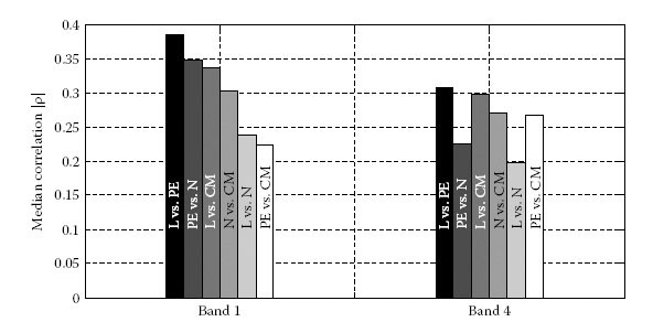
FIGURE 5.21
Median noise correlation between different Rx ports, for Band 1 and Band 4.

$H=\left(\begin{array}{ccc}{h}_{11}& \dots & h_{1N_T}\\ ⋮& \ddots & ⋮\\ h_{N_{R}1}& \cdots & h_{N_R{N}_T}\end{array}\right).$

(5.2)

The singular value decomposition (SVD), which was already introduced in Chapter 4, decomposes the channel matrix H into three matrices:

$H=UD{V}^H,$

(5.3)

where

^H is the Hermitian operator (transpose and conjugate complex)

D is a diagonal matrix containing the singular values $\sqrt{{\text{λ}}_j}\left(j=1,\dots ,r\right)$ of the channel matrix H in decreasing order; r is the rank of H

The number of non-zero singular values is derived from the number of transmit and receive ports as r = min(N_T, N_R) if H has full rank. In practice, this condition is always fulfilled (see the results for the spatial correlation later). U and V are unitary matrices, that is, U⁻¹ = U^H and V⁻¹ = V^H. The SVD decomposes the channel matrix into parallel and independent SISO branches as denoted by the diagonal structure of D.

Since U and V are unitary matrices, multiplication by these matrices preserves the total energy. The singular values $\sqrt{{\text{λ}}_j}$ of D describe the attenuation of the decomposed SISO branches (note that the channel matrix H was not normalised before calculating the SVD). The decomposition into parallel and independent spatial streams by the SVD is very useful in MIMO theory and will be used and discussed later in more detail, for example, in Chapters 8 and 9.

FIGURE 5.22
Attenuation of the singular values of the first MIMO stream.

Figure 5.22 shows the probability (bar graphs) and the cumulative probability (line graphs) of the attenuation of the first singular value $-20*{\log }_{10}\left(\sqrt{{\text{λ}}_1}\right)$ (first MIMO stream) for different MIMO configurations. The underlying data of this plot are all the MIMO measurement channels (346 in total) of all buildings, countries and all frequencies. Each bar graph from left to right shows the MIMO configurations depicted in the legend (from top to down). As explained earlier, the number of the used transmit and receive ports define the number of MIMO streams: One spatial stream is available if only one transmit port is used; two spatial streams can be used for transmission if two transmit ports and more than two receive ports are used.Figure 5.23 shows a zoom plot of Figure 5.22 at the high coverage area. Figure 5.24 illustrates the corresponding attenuation of the second singular value where a second spatial stream is available, that is, for the 2 × 2 (⊲) and 2 × 4 (⊳) configuration. Increasing the number of transmit and receive ports results in a lower attenuation of the spatial streams. A comparison between the 2 × 4 MIMO configuration (⊳) and SISO (1 × 1 configuration, ◽) shows the MIMO gain. The first 2 × 4 stream is 11 dB less attenuated at the 50% point (median) than the SISO path. Additionally, the second stream supports data transmission. The attenuation of the second stream (2 × 4 (⊳) in Figure 5.24) is 3 dB higher compared to SISO (in Figure 5.22). The zoom at high attenuations reveals even a higher gain of MIMO. Considering the 90% percentile the first stream is 13 dB less attenuated than the SISO path while the attenuation of the second stream is only 1.5 dB higher compared to SISO. Thus, MIMO improves in particular the performance of highly attenuated channels which are most important to meet coverage requirements.

The relation between the MIMO paths can be attributed by the spatial correlation which is an important measure of the MIMO channel. The spatial correlation affects not only the channel capacity (see Chapter 9) but also the performance of different MIMO schemes (see Chapters 8 and 9). Note that a discussion on the spatial correlation of the MIMO PLC channel can be also found in Chapter 4. The condition number of a matrix can be used as a measure of the spatial correlation. The condition number is defined as the ratio of the largest singular value to the smallest singular value:

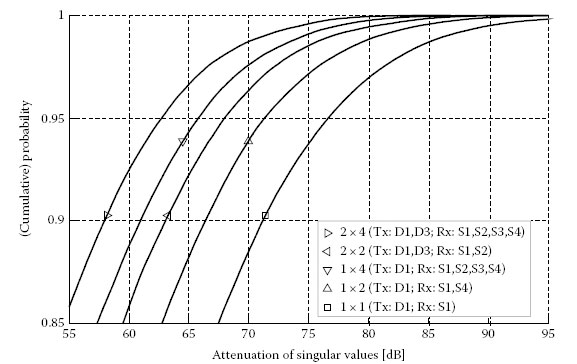
FIGURE 5.23
Attenuation of the singular values of the first MIMO stream: zoom.

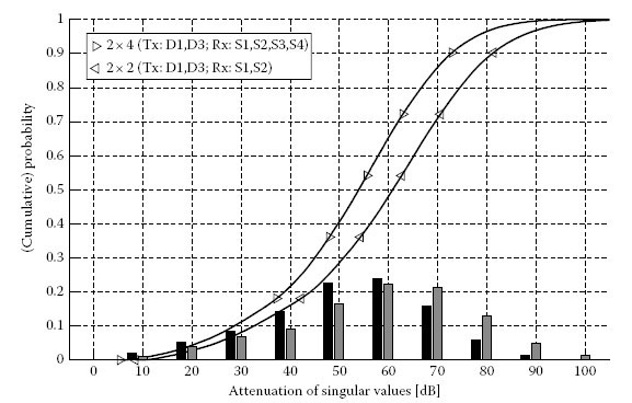
FIGURE 5.24
Attenuation of the singular values of the second MIMO stream.

$20*{\log }_{10}\left(\frac{\sqrt{{\text{λ}}_1}}{\sqrt{{\text{λ}}_2}}\right).$

(5.4)

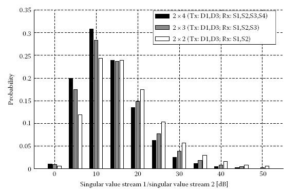
FIGURE 5.25
Spatial correlation.

As explained earlier, the singular values describe the attenuation of the MIMO streams. The attenuation fraction of the channel is reduced by calculating the ratio according to Equation 5.4. The higher the condition number according to Equation 5.4, the higher the attenuation of the second stream compared to the first stream and the higher the spatial correlation. The definition of the spatial correlation is illustrated by the extreme case of a fully correlated MIMO channel where all the channel coefficients of the channel matrix H have the same value. As a consequence, the rank of this channel matrix is one, the second singular value is equal to zero, and thus the spatial correlation according to Equation 5.4 approaches infinity.Figure 5.25 shows the probability of the spatial correlation according to the definition of Equation 5.4 for the 2 × 2, 2 × 3 and 2 × 4 MIMO configurations. The rare occurrence of high values of the condition number indicates a rather high spatial correlation of the MIMO PLC channel. The 2 × 4 MIMO configuration comprises in 60% of the channels and frequencies a spatial correlation of >10 dB. Although the second stream is significantly attenuated compared to the first stream in this case, it has to be kept in mind that the first stream is significantly less attenuated compared to SISO. The MIMO performance is gained by the combination of both spatial streams and not only by the availability of the second stream (see also the channel capacity results in Chapter 9).

5.3    Statistical Modelling of the PLC MIMO Channel Based on Experimental Data

5.3.1    MIMO CTF Modelling

In this section, a step-by-step description is given for the statistical modelling of the PLC MIMO channel transfer function (CTF) based on experimental measurements. The purpose of the model is to capture the main physical features of the transmission channel, including its median attenuation, its frequency domain path loss characteristics, its multipath and frequency fading structure and the correlation between different MIMO paths. These parameters were characterised from experimental measurements in Section 5.2.1. The proposed model is statistical in nature, and will be developed following a top-down approach. Therefore, its purpose is not to reproduce exactly the CTF measured at a given measurement location, but rather to enable the generation of random CTF exhibiting similar statistics in line with actual channel measurements.

The philosophy used in the modelling process has been first presented in [10]. In this first proposal, the model parameters were extracted from a limited set of measurements performed in five houses in France, leading to a collection of 42 CTF matrices. Measurements were taken using differential ports at both the Tx and Rx. Hence, 3 × 3 MIMO channel matrices were generated by the model.

In the present study, a larger set of data is considered, as measurements have been taken in 36 buildings in six different countries: Belgium, France, Germany, Italy, Spain and United Kingdom. Differently from the analysis in [10], the couplers used for this measurement series used differential ports at the Tx (D1: line–neutral port, D2: neutral–protective earth port and D3: protective earth–line port), and star-style ports at the Rx (S1: line port, S2: neutral port and S3: protective earth port). In addition, a fourth Rx port (S4) was available to receive CM signals flowing through the three wires. More details on MIMO coupling can be found in Chapter 1. The corresponding MIMO configuration is called 3 × 4 MIMO, and therefore, each measured CTF between any two outlets consists of a 4 × 3 matrix, as shown in Figure 5.26. The overall measurement set comprises 351 4 × 3 CTF matrices. More details about the measurement campaign and the corresponding channel characterisation analysis can be found in Section 5.2.

As explained in Section 5.2.1, no significant difference between the channels measured in different countries was observed. Highly attenuated channels as well as channels with better propagation conditions could be found in each country. Therefore, the following model will capture the global measurement statistics independently from the country where the measurement was taken. The output will be representative of the PLC channel transmissions conditions in Europe.

5.3.1.1    Median Channel Gain Modelling

A first important feature representative of the PLC CTF is the median channel gain, since it governs the overall signal attenuation to be expected by a transmission system. In this analysis, the median gain of the CTF is defined as a matrix A providing the median value across frequency for each element of the channel matrix H(f):

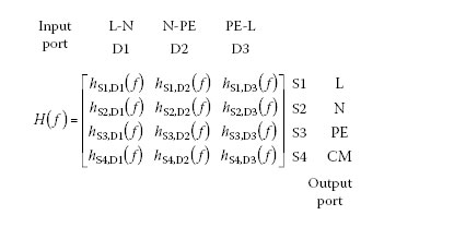
FIGURE 5.26
Description of the measured and modelled channel matrix: input and output ports.

$A=\left[\begin{array}{ccc}{A}_{\text{S}1,\text{D1}}& A_{\text{S}1,\text{D2}}& A_{\text{S}1,\text{D3}}\\ A_{\text{S2},\text{D1}}& A_{\text{S2},\text{D2}}& A_{\text{S2},\text{D3}}\\ A_{\text{S3},\text{D1}}& A_{\text{S3},\text{D2}}& A_{\text{S3},\text{D3}}\\ A_{\text{S4},\text{D1}}& A_{\text{S4},\text{D1}}& A_{\text{S4},\text{D3}}\end{array}\right]=med\left(\left|H\left(f\right)\right|\right),$

(5.5)

where med() represents the element-wise median operator. Complementarily, the representation of the median channel gain in dB will be denoted A_dB:

$A_{\text{dB}}=20\cdot {\log }_{10}\left(A\right)=med\left(10\cdot {\log }_{10}\left({\left|H\left(f\right)\right|}^2\right)\right).$

(5.5)

As a first step, the statistics of the median gain of the D1–S1 link, A_S1,D1, is investigated. The solid line in Figure 5.27 represents the CDF of this parameter in dB. One can observe that this median gain varies between −80 dB for the most attenuated channels and −10 dB for weakly attenuated channels. This observation is comparable to the results in Figure 5.2, where the CDF of the channel attenuation over all frequencies for a given feeding style is provided. In addition, the shape of the CDF shows that the distribution of parameter A_{dB S1,D1} is close to a Gaussian distribution. The dashed curve represents the fitted Gaussian approximation, with mean μ_A = −50.1 dB and standard deviation σ_A = 15.6 dB. Therefore, the first parameter of the model is A_{dB S1,D1}, and will be randomly selected according to the following normal distribution:

$A_{\text{dB}\text{S1,D1}}=N\left({\text{μ}}_A,{\text{σ}}_A\right),$

(5.7)

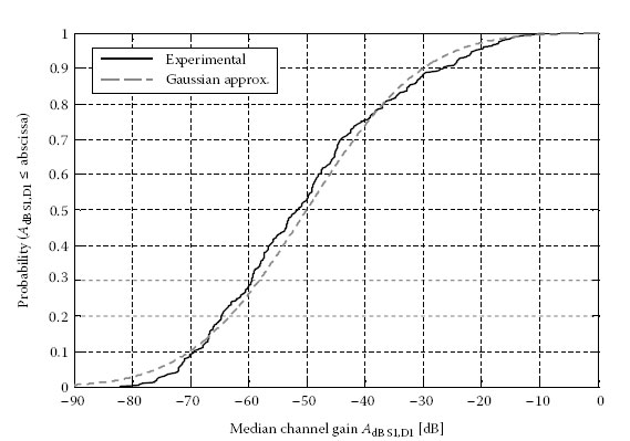
FIGURE 5.27
CDF of the median gain of the D1–S1 link A_{dB S1,D1}.

where the probability density function (PDF) of the normal distribution $N\left(\text{μ,σ}\right)$ is given by

$p_X\left(x\right)=\frac{1}{\sqrt{2\text{π}}\text{σ}}\exp \left(-\frac{{\left(x-\text{μ}\right)}^2}{2{\text{σ}}^2}\right).$

(5.8)

In order to characterise the other elements in matrix A_dB, that is, the median gain of the other links in the MIMO channel matrix, it is interesting to analyse how they are related to parameter A_{dB S1,D1}. For this purpose, Figure 5.28 provides scatter plots of the observed values of A_{dB S2,D1} and A_{dB S3,D1}, respectively, versus the value of A_{dB S1,D1}, for the 351 measured channel matrices. As a reminder, A_{dB S2,D1} provides the median channel gain for the D1–S2 link and A_{dB S3,D1} provides the median channel gain for the D1–S3 link. As can be seen on these graphs, the median gain parameters are highly similar, as the plots approximately align along the y = x line (dotted line).A similar observation was made in the characterisation phase: in Figure 5.3, it is shown that the channel attenuation is similar when considering either the S1, S2 or S3 receive ports. In Figure 5.28, the difference between the plotted parameters can be seen as a deviation with respect to perfect equality. By comparing Figure 5.28a and b, one can conclude that the deviation between A_{dB S3,D1} and A_{dB S1,D1} is larger than the deviation between A_{dB S2,D1} and A_{dB S1,D1}. This can be physically interpreted, since the output ports S1 (L wire) and S2 (N wire) both comprise a wired connection to the differential input port D1 (L-N), and are symmetrical with respect to each other. On the contrary, the output port S3 corresponds to the PE wire which is not wired to the input port D1. This can explain the larger deviation.

Similar characteristics were observed for all input ports D1, D2 and D3, and for the three output ports S1, S2 and S3. Therefore, it is proposed to model parameters A_{dB Sm, Dn} for m ∈ [1,2,3] and n ∈ [1,2,3] as

$A_{\text{dB}\text{S}m\text{,D}n}=A_{\text{dB}\text{S1,D1}}+N\left(0,{\text{σ}}_{\text{S}m,\text{D}n}\right),$

(5.9)

where the deviation between parameter A_{dB S1,D1} and parameter A_{dB Sm, Dn} is modelled as a Gaussian distribution with mean 0 and standard deviation σ_Sm,Dn. This last parameter can be easily derived from experimental measurements by computing the standard deviation of the difference between A_{dB Sm,Dn} and A_{dB S1,D1}, as will be done in the following paragraphs.

A closer look needs now to be taken at the median channel gain parameter A_{dB S4,Dn} when the output port S4 is involved, that is, using CM reception.Figure 5.29 provides similar scatter plots as Figure 5.28 for parameters A_{dB S4,D1} and A_{dB S4,D3}, respectively.

In both cases, one can observe that the approximation given in Equation 5.9 is no longer valid. Indeed, the scatter plot is no longer aligned with the dotted y = x line. For highly attenuated channels (bottom-left corner of the graph), reception using the CM tends to generate a lower attenuation, while for low attenuated channels (top-right corner of the graph), the attenuation is stronger when receiving using the CM (S4 port). This particularity was already observed when statistically analysing the experimental measurements (see Figures 5.3 and 5.5). A linear regression analysis showed that these scatter plots are much better aligned with the line given by y = 0.5x−30 (solid line). The same result holds for parameter A_{dB S4,D3} (data not shown). Therefore, a refined model will be used when considering MIMO links involving CM reception on port S4, as follows (n ∈ [1,2,3]):

$A_{\text{dB}\text{S4,D}n}=0.5\times A_{\text{dB}\text{S1,D1}}-30+N\left(0,{\text{σ}}_{\text{S4},\text{D}n}\right),$

(5.10)

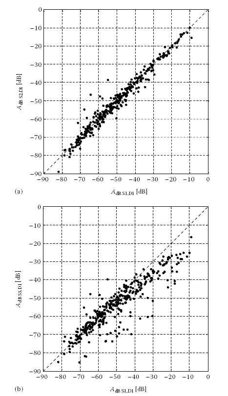
FIGURE 5.28
Scatter plots of median channel gains: (a) A_{dB S2,D1} versus A_{dB S1,D1} and (b) A_{dB S3,D1} versus A_{dB S1,D1}.

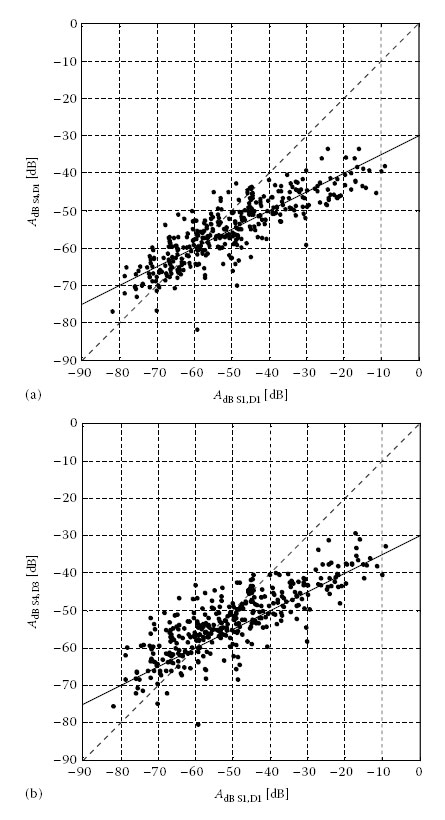
FIGURE 5.29
Scatter plots of median channel gains: (a) A_{dB S4,D1} versus A_{dB S1,D1} and (b) A_{dB S4,D3} versus A_{dB S1,D1}.

where values 0.5 and −30, respectively, represent a slope and an y-intercept accounting for the particular shape of the scatter plot observed in Figure 5.29. The deviation from this linear model is given by a Gaussian distribution with mean 0 and standard deviation σ_S4,Dn. The values of σ_S4,Dn can be easily derived from observations of experimental measurements. All values of the standard deviations σ_Sn,Dn in dB are grouped in a single matrix as follows:

$\left[{\text{σ}}_{\text{S}m,\text{D}n}\right]=\left[\begin{array}{ccc}0& 5.1& 3.8\\ 2.9& 5.7& 5.2\\ 6.6& 7.8& 6.9\\ 4.6& 5.9& 5.1\end{array}\right]\text{in}\text{dB}\text{.}$

(5.11)

5.3.1.2    Frequency Domain Path Loss Modelling

Once the median channel gain is settled, the focus is now placed on the modelling of the frequency domain path loss. For this purpose, the proposed MIMO channel model builds on a widely accepted SISO PLC channel model first developed by Zimmerman [11]. This model accounts for both the multi-path characteristics of the PLC channel and its particular frequency domain power decay. The same formalism was used within the ICT OMEGA Project [12]. This CTF model H(f) is mathematically described as follows:

$H\left(f\right)=A{\displaystyle \sum _{p=1}^{N_p}{g}_p{e}^{-j\left(2\text{π}{d}_p/v\right)f}{e}^{-\left(a_0+a_1{f}^k\right)d_p}},$

(5.12)

where

v represents the speed of the electromagnetic wave in the copper wire

d_p and g_p, respectively, represent the length and gain of the propagation path

N_p represents the number of propagation paths

The other parameters a₀, a₁, K and A are attenuation factors

An interesting statistical extension of this model was proposed by Tonello in [13] and further developed in [12]. This extension assumes that the multiple paths are generated by a Poisson arrival process with intensity Λ, and L_max denotes the maximum length of the signal paths. In addition, the gains g_p of the propagation paths are considered to be uniformly distributed in the range [−1, 1]. Under these assumptions, Tonello computed the statistical expectation of the frequency domain path loss as

$PL\left(f\right)=A^2\frac{\text{Λ}}{3}\frac{1-e^{-2L_{max}\left(a_{à}+a_1{f}^k\right)}}{\left(2a_0+2a_1{f}^k\right)\left(1-e^{-\text{Λ}{L}_{max}}\right)}.$

(5.13)

Note that in this model, parameter A governs an arbitrary attenuation of the channel. Therefore in the following, we will consider it as the experimental median gain of the measured channels as described in Section 5.3.1.1. The expression of the expected path loss provided by Equation 5.13 is useful to derive parameters a₀, a₁ and K from experimental measurements. For this purpose, parameter A was taken as the median gain for each measurement, and parameters L_max and Λ were arbitrarily fixed to 800 m and 0.2 m⁻¹ as it is done in [12]. By selecting L_max = 800 m, one considers that the signals travelling along propagation paths (including multiple reflections) longer than 800 m do not play a significant role in the structure of the path loss. This assumption is reasonable due to the strong attenuation of signals with increasing distance. The choice of Λ = 0.2 m⁻¹ implies that the average excess length between any two successive propagation paths is 5 m. This means that the average distance between any two successive junctions or outlets in the electrical network is 2.5 m. This value is in line with observed wiring practices for indoor electrical networks.

The values of a₀, a₁ and K can then directly be obtained for each measurement using a simulated annealing procedure. This method requires input parameters, and the values defined in the OMEGA Project were used, namely a_0,init = 3 × 10⁻³, a_l,init = 4 × 10⁻¹⁰ and K_init = 1.Figure 5.30 presents an example of such a fitting, performed on an experimental CTF measured for the D1–S1 link in a German house. For this particular example, the simulated annealing procedure resulted in the following path loss parameters: a₀ = 3.6 × 10⁻⁴, a₁ = 4 × 10⁻¹⁰ and K = 1.04.

Path loss parameters were obtained for the 12 possible links for each of the 351 measured MIMO channel matrices. As a result, 4212 values were available for the statistical evaluation of each of the path loss parameters. As a first observation, no particular dependency of the path loss parameters with the particular link considered within the MIMO matrix was detected. Therefore, the statistical distribution of each parameter was considered globally from the 4212 samples. Figure 5.31 provides the experimental estimate of the PDF for parameter a₀, obtained using a normalised histogram. It can be observed that the PDF of a₀ follows an exponential decay with negative minimum values. Hence, it is proposed to model this parameter using a shifted exponential distribution E_shift(μ_a0,δ_a0). The PDF of the shifted exponential distribution E_shift(μ,τ) is defined as

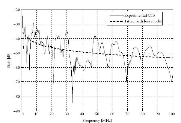
FIGURE 5.30
PLC CTF measured in a German house, and fitted path loss model..

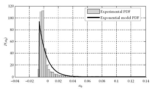
FIGURE 5.31
Experimental PDF versus shifted exponential model PDF for variable a₀.

$p_X\left(x\right)=\frac{1}{\text{γ}}\exp \left(-\frac{x-\text{δ}}{\text{γ}}\right).$

(5.14)

Figure 5.31 also represents the shifted exponential model PDF for variable a₀, where the best fitting parameters are given by μ_a0 = 1.04 × 10⁻² and δ_a0 = −6.7 × 10⁻³. These parameters will be used to randomly generate realistic values for parameter a₀. The same statistical distribution was already observed in [10], with similar parameter values.

Parameter a₁ will be much more easily modelled. Indeed, for 97% of the measured channels, the estimated value of a₁ stayed equal to the input value of a_l,init = 4 × 10⁻¹⁰. Therefore, this value will be constant in the proposed model, as was already done in [10].

Finally, Figure 5.32 represents the experimental estimate of the PDF for parameter K, in the form of a normalised histogram. This experimental PDF takes a slightly asymmetric shape, which is in general well represented using a heavy-tailed distribution. The Weibull distribution W(α, β) is an example of such heavy-tailed distributions that can be adapted to experimental data by fitting its parameters α and β. The Weibull distribution PDF is given by

$p_X\left(x\right)=\text{αβ}\cdot x^{\text{β}-1}\exp \left(-\text{α}\cdot x^{\text{β}}\right).$

(5.15)

The Weibull distribution best fitting the experimental distribution of parameter K was obtained with parameters α_K = 5.7 × 10⁻² and β_K = 57.7. Its theoretical PDF is represented in Figure 5.32, and will be used to randomly generate values of parameter K for the MIMO channel model. It can be noted that in [10], a normal distribution was selected, with a similar mean value. In the present work, the larger dataset allowed to refine this estimate, in particular by accounting for the distribution asymmetry. Table 5.2 summarises the statistical models of the path loss parameters.

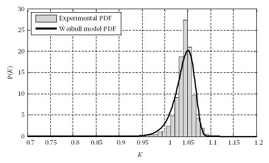
FIGURE 5.32
Experimental PDF versus Weibull model PDF for variable K.

TABLE 5.2

Statistical Models of the Path Loss Parameters

Path Loss Parameter	Model	Parameters
AdB S1,D1	N(μA, σA)	μA=−50.1dB
		σA = 15.6 dB
AdB Sm,Dn(m ∈[1,2,3])	AdB Sm,Dn = AdB S1,D1 + N(0, σSm,Dn)
AdB S4,Dn	AdB S4,Dn=0.5 ×AdB S1,D1–30+N(0, σS4,Dn)	$\left[{\text{σ}}_{\text{S}m,\text{D}n}\right]=\left[\begin{array}{ccc}0& 5.1& 3.8\\ 2.9& 5.7& 5.2\\ 6.6& 7.8& 6.9\\ 4.6& 5.9& 5.1\end{array}\right]\text{dB}$
a0	$E_{shift}\left({\text{μ}}_{a0},{\text{δ}}_{a0}\right)$	${\text{μ}}_{a0}=1.04\times {10}^{-2}$
		${\text{δ}}_{a0}=-6.7\times {10}^{-3}$
a1	Constant	a1 = 4 × 10−10
K	W(αK, βK	αK = 5.7 × 10−2
		βK = 57.7
Lmax	Constant	Lmax = 800 m
Λ	Constant	Λ = 0.2 m−1

Note:  Parameters a₀, a₁ and K are dimensionless.

5.3.1.3    Multi-Path Model for the SISO Line–Neutral (D1) to Line (S1) Path

Once the path loss parameters of the MIMO channel model are settled, the modelling procedure focuses on the multi-path and frequency fading structure of the PLC channel. Statistical channel models dedicated to SISO links already exist, where this specific feature is well captured. In particular, the proposed MIMO channel model builds on the SISO channel framework developed by Zimmermann and Tonello in [11,14]. More specifically, the first step in the MIMO channel model consists in emulating the line–neutral to line path (D1–S1 link) using Equation 5.12, where the generic parameter A is replaced with A_S1,D1, and the path loss parameters A_S1,D1, a₀, a₁ and K are selected according to the statistical distributions specified in Table 5.2. Following [12], the path lengths d_p are randomly generated as events of a Poisson arrival process P(Λ) characterised by its intensity Λ. Using a maximum path length L_max, the Poisson process also leads to a finite number of paths N_p. Note that the values of Λ and L_max are fixed and provided in Table 5.2. Finally, the gains g_p of the propagation paths are generated using a uniform statistical distribution U(g_min, g_max) within the range [−1,1].

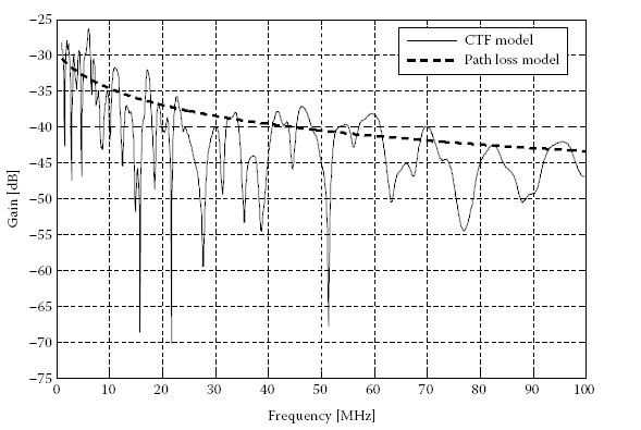
FIGURE 5.33
PLC CTF generated using the SISO model, and corresponding path loss model.

Figure 5.33 presents a CTF of a D1–S1 link generated using the proposed channel model. The corresponding path loss model is also represented. One can notice its similarity with measured CTF such as the one presented in Figure 5.30.

5.3.1.4    Extension of the Multi-Path Model to the MIMO Channel Matrix

In order to extend the SISO channel model to the full MIMO matrix, it is first necessary to investigate the characteristics of the last feature that the model intends to capture, namely the correlation between different MIMO links. As explained in Section 5.2.4, the degree of correlation within the MIMO channel matrix has an impact on the channel capacity and on the performance of MIMO signal processing techniques (see also Chapter 9). In order to capture the frequency fading correlation between individual channels in the MIMO matrix, this study uses the Pearson correlation coefficient ρ already introduced in [10]. It is recalled that the computation of this coefficient requires evaluating the statistical expectation of the channel gain. As we are interested only in the correlation of the fast fading behaviour of the CTF, the Pearson correlation coefficient ρ will be computed on a normalised CTF defined as follows:

${\tilde{h}}_{\text{S}m,\text{D}n}\left(f\right)=\frac{h_{{}_{\text{S}n,Dm}}\left(f\right)}{\sqrt{P{L}_{{}_{\text{S}n,\text{D}m}}\left(f\right)}},$

(5.16)

where

h_Sn,Dm(f) represents the CTF between input port Dm and output port Sn

PL_Sn,Dm(f) represents its expected path loss computed using Equation 5.13

This normalised CTF is Wide Sense Stationary and thus the statistical expectations used in the computation of the correlation coefficient can be replaced by the frequency domain average. The complex correlation coefficient between channel h_Sn,Dm(f) and channel h_Si,Dj(f) in the MIMO matrix is finally computed using the following equation:

${\text{ρ}}_{\text{S}n\text{D}m,\text{S}i\text{D}j}=\frac{\langle {\tilde{h}}_{\text{S}n,\text{D}m}\left(f\right){\tilde{h}}_{\text{S}i,\text{D}j}^{*}\left(f\right)\rangle -\langle {\tilde{h}}_{\text{S}n,\text{D}m}\left(f\right)\rangle \langle {\tilde{h}}_{\text{S}i,\text{D}j}^{*}\left(f\right)\rangle }{\sqrt{\left(\langle {\left|{\tilde{h}}_{\text{S}n,\text{D}m}\left(f\right)\right|}^2\rangle -{\left|\langle {\tilde{h}}_{\text{S}n,\text{D}m}\left(f\right)\rangle \right|}^2\right)\left(\langle {\left|{\tilde{h}}_{\text{S}i,\text{D}j}\left(f\right)\right|}^2\rangle -{\left|\langle {\tilde{h}}_{\text{S}i,\text{D}j}\left(f\right)\rangle \right|}^2\right)}},$

(5.17)

where

$\langle \rangle$ denotes the frequency domain average

* denotes the complex conjugate operator

Note that Equation 5.17 provides a correlation coefficient independent of frequency, by comparing the variations of any two channels across their measurement frequency range. Computation of frequency-dependent correlation factors is also possible but requires considering all channels in a measurement matrix simultaneously (see, for instance, the study presented in Chapter 4).

The correlation coefficient ρ_SnDm, _SiDj was computed for each of the 351 measured channel matrices, and for each possible pair of MIMO links. As the measurements were performed using three possible Tx ports (D1 to D3) and four possible Rx ports (S1 to S4), the MIMO channel matrix contains 12 possible links, and thus 66 pairs of distinct channels can be considered.Figure 5.34 provides the statistical CDF of coefficient ρ for a number of specific cases. As a first observation, the statistical distribution of coefficient ρ can be analysed over the whole set of channel pairs (Δ marker). One can notice that the correlation coefficient is ranging all values between 0 and 1, with a quasi-uniform distribution. Hence, both correlated channels ($\left|\text{ρ}\right|$ > 0.8) and uncorrelated channels ($\left|\text{ρ}\right|$ < 0.2) could be measured. In order to get more insights in the nature of the correlation between MIMO links, Figure 5.34 also represents the correlation coefficient CDF for subsets of the measurement ensemble, namely

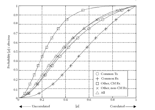
FIGURE 5.34
Statistical CDF of the correlation coefficient ρ obtained from experimental measurements.

•  All channel pairs using the same Tx port (○ marker)

•  All channel pairs using the same Rx port (+ marker)

•  All channel pairs with different Tx and Rx port, where one channel uses the CM (S4) Rx port (◽ marker)

•  All channel pairs with different Tx and Rx port, where the CM (S4) Rx port is not used (× marker)

Observations of the resulting CDF reveal that using the same Tx port does not increase the correlation between channels significantly. However, two channels using the same Rx port are more correlated than average, as the corresponding CDF curve moves towards the right-hand side of the figure. When considering channel pairs that do not share the same Tx port nor the same Rx port, it appears that the correlation coefficient is similar to the average when the CM port is not used. Nevertheless, employing the CM Rx port provides a channel that is less correlated to any other channel using different ports. This could be expected from physical considerations, as CM reception involves unique transmission mechanisms that can differ from classical wire reception.

From this evaluation of the correlation characteristics of the MIMO channel matrix, a full MIMO PLC channel model can be developed. The SISO D1–S1 link is already modelled using the procedure described in Section 5.3.1.3. All other links in the MIMO channel matrix will be modelled using an extended CTF definition as follows:

$H\left(f\right)=A{\displaystyle \sum _{p=1}^{N_p}{g}_p{e}^{-j{\phi }_p}{e}^{-j\left(2\text{π}{d}_p/v\right)f}{e}^{-\left(a_0+a_1{f}^k\right)d_p}}.$

(5.18)

In this CTF equation, each path was assigned an arbitrary additional phase φ_p. The idea originally developed in [10] is to randomly select the value φ_p for each path using a uniform distribution U(–Δφ/2, Δφ/2) within a given range [–Δφ/2, Δφ/2]. The larger the value of Δφ, the less correlated the resulting channel will be with respect to the line–neutral to line SISO path. For an extreme value of Δφ = 2π, a low level of correlation is expected for the corresponding channel. On the contrary, selecting a value of Δφ = 0 will produce a channel identical to the reference channel, with a correlation coefficient ρ = 1. In order to keep the degree of correlation observed for channels involving the L, N or PE Rx ports, it is proposed to modify only two parameters when generating different links within the MIMO matrix: the median gain A and the vector of arbitrary phases $\left\{{\text{φ}}_p,p=1,\dots ,N_p\right\}$. This choice is consistent with the physical observation that the topology of the electrical network is the same, independently from the considered MIMO link. Therefore, it seems reasonable to keep parameters such as the distribution of path lengths $\left\{d_p,p=1,\dots ,N_p\right\}$ or path gains $\left\{g_p,p=1,\dots ,N_p\right\}$ constant when considering L, N or PE reception. An exception is made for CM reception (port S4): as observed in Figure 5.34, those channels present a lower degree of correlation with channels using different Rx ports. Therefore, for CM reception, a specific distribution of path lengths $\left\{d_{\text{S}4,p},p=1,\dots ,N_{p,\text{S}4}\right\}$ will be generated using the same Poisson arrival process P(Λ) as for the LN-N path. Complementarily, a new set of path gains $\left\{g_{\text{S}4,p},p=1,\dots ,N_{p,\text{S}4}\right\}$ will be drawn from a uniform distribution U(g_min, g_max) within the range [−1, 1].

TABLE 5.3

Statistical Models of the MIMO Multi-Path Parameters

MIMO Multi-Path
Parameter	Model	Parameters
$\left\{d_p,p=1,\dots ,N_p\right\}$	P(Λ)	Λ= 0.2 m−1
		Lmax = 800m
$\left\{g_p,p=1,\dots ,N_p\right\}$	$U\left(g_{min},g_{max}\right)$	gmin = −1V
		gmax = 1V
$\left\{d_{\text{S}4,p},p=1,\dots ,N_{p,\text{S}4}\right\}$	P(Λ)	Λ= 0.2 m−1
		Lmax = 800m
$\left\{g_{\text{S}4,p},p=1,\dots ,N_{p,\text{S}4}\right\}$	$U\left(g_{min},g_{max}\right)$	gmin = −1V
		gmax = 1V
v	Constant	v = 2 × 108 m/s
$\left\{{\text{φ}}_p,p=1,\dots ,N_p\right\}$	$U\left(-\Delta \text{φ}/2,-\Delta \text{φ}/2\right)$	Δσ = 2π rad to generate links D1-S2 and D1–S3 from link D1–S1
		Δσ = 4π/3 rad to generate links D2–Sm and D1–Sm from links D1–Sm (m = 1, 4)

Note:  Parameters g_min and g_max are normalised voltages.

In order to select the appropriate values of Δφ, Monte Carlo simulations were run and the resulting channel correlation factors were compared to the experimental observations. The following values are finally recommended:

•  To generate link D1–S2 from link D1–S1, and link D1–S3 from link D1–S1, select Δφ = 2π.

•  For m = 1, …, 4, to generate link D2–Sm from link D1–Sm, and link D3–Sm from link D1–Sm, select Δφ= 4π/3.

Table 5.3 summarises all necessary parameters for the simulation of random 3 × 4 MIMO channel matrices.

5.3.1.5    Evaluation of the Channel Model

Figure 5.35 provides an example of generated CTF using the proposed statistical MIMO PLC channel model. The channel model generally produces 3 × 4 channel matrices, but for the sake of legibility, only the four channels corresponding to the line–neutral differential port (D1) at Tx are represented. One can note that the model produces random MIMO CTFs that faithfully replicates the multi-path structure observed for experimental measurements (see Section 5.2.2). By construction, the channel model also reproduces the statistics observed for the main path loss parameters, namely the median channel gain A and the frequency domain power decay parameters a₀, a₁ and K.

Finally, it is interesting to analyse how the proposed MIMO channel model renders the correlation between different links within the MIMO matrix. For this purpose, a random draw of 351 3 × 4 MIMO channel matrices was generated. From this synthetic data set, the correlation coefficient ρ between any two links within each MIMO matrix was computed using the same method already described in Section 5.3.1.4. The CDF of the magnitude of ρ is displayed in Figure 5.36 for the same specific cases as for the experimental data set: for channels sharing the same Tx port, for channels sharing the same Rx port, for channels without any port in common and using the CM Rx port, and for channels without any port in common and using the L, N or PE port at Rx. By comparing Figures 5.34 and 5.36, one can observe similar correlation trends between the proposed model and the experimental measurements. In particular, the larger correlation between channels sharing the same Rx port is well reproduced. Second, the low correlation between channels involving the CM port and other channels is well captured. Finally, all other channels present an average correlation, spanning the [0,1] interval in a quasi-uniform way.

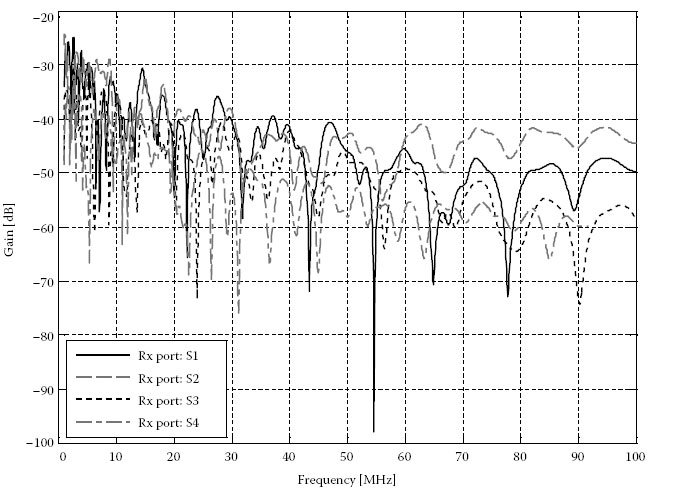
FIGURE 5.35
Example of PLC CTF generated using the proposed MIMO model (Tx port: D1 only).

5.3.2    Multiple-Output Noise Modelling

5.3.2.1    Multivariate Time Series

A complete and detailed noise model can be achieved through both frequency domain and time domain modelling techniques. However, in a multiple-output noise model, one of the most important features one wishes to capture is the correlation between the signals received at different ports. Characteristics of the experimentally observed noise correlation are exposed in Section 5.2.3.2. On the other hand, the multi-path structure of the received signals, that produce fading notches in the frequency domain, can also be seen as the correlation between successive samples in the time domain. Hence, modelling of the multiple-output noise will present less complexity and more effectiveness in the time domain.

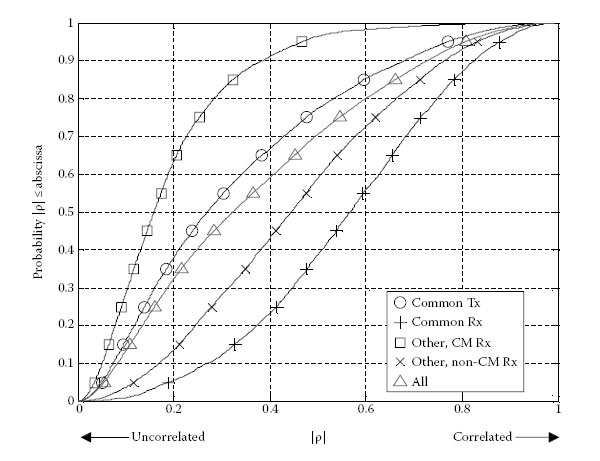
FIGURE 5.36
Statistical CDF of the correlation coefficient ρ obtained from model simulations.

Multivariate time series (MTS) analysis is a powerful mathematical technique used for the modelling and forecasting of the future values of time sequences. The mathematical framework usually employed for the modelling of MTS is the vector autoregressive (VAR) model. The suitability and utility of MTS modelling in the context of MIMO PLC noise has been first demonstrated in [15] where it was applied to a small series of noise measurements conducted in French homes. The method is described in the following sections through its application to the ETSI noise measurements presented in Section 5.2.3.

The time domain noise, as mentioned in Section 5.2.3, is measured on four ports simultaneously: S1, S2, S3 and S4. This noise can be visualised as a four-variate time series which is a special case of MTS. A MTS is an ensemble of individual time sequences measured at fixed and equally spaced time intervals Δt. A MTS consists of simultaneous observations of several variables. Consider a MTS $\left\{N_t\right\}$ with n variables such that $N_t={\left(x_{1t},\dots ,x_{nt}\right)}^T$, where T stands for transpose. A four-variate MTS consists of $\left\{x_{1t}\right\}$, $\left\{x_{2t}\right\}$, $\left\{x_{3t}\right\}$ and $\left\{x_{4t}\right\}$. The measured noise can be characterised as an MTS with n = 4 and a sampling period Δt = 2 ns. It should be noted that $\left\{x_{1t}\right\}$, $\left\{x_{2t}\right\}$, $\left\{x_{3t}\right\}$ and $\left\{x_{4t}\right\}$ represent S1, S2, S3 and S4 noise, respectively. For analysis, we consider the duration of the vector as 46.52 μs which is equal to the duration of an OFDM symbol in the HomePlug AV2 standard for commercial PLC devices (see Chapter 14).

5.3.2.2    Figures of Merit for Model Validation

Each noise measurement is an ensemble of four noise series; therefore, their spectra need to be observed individually. The overall spectral form of the noise is of a decreasing exponential function as shown in Figure 5.11. At this point, we define a parameter ψ_i,j, shown in Equation 5.19, which denotes frequency domain cross-correlation between the measured noise PSD and the modelled noise PSD (for any of S1, S2, S3 and S4 measurements). The parameter ψ_i,j, serves as a figure of merit of spectral resemblance between the measured and modelled noise:

${\text{ψ}}_{i,j}=\frac{\overline{N_i\left(f\right)N_j^{*}\left(f\right)}-\overline{N_i\left(f\right)}\overline{N_j^{*}\left(f\right)}}{\sqrt{\left(\overline{N_i{\left(f\right)}^2}-{\overline{N_i\left(f\right)}}^2\right)\left(\overline{N_j{\left(f\right)}^2}-{\overline{N_j\left(f\right)}}^2\right)}},$

(5.19)

where

N(f) represents the envelope of the noise PSD in dBm/Hz

Subscripts i and j stand for the measured and modelled noise, respectively

$\begin{array}{l}{\text{ψ}}_{i,j}=\frac{\overline{N_i\left(f\right)N_j^{*}\left(f\right)}-\overline{N_i\left(f\right)}\overline{N_j^{*}\left(f\right)}}{\sqrt{\left(\overline{N_i{\left(f\right)}^2}-{\overline{N_i\left(f\right)}}^2\right)\left(\overline{N_j{\left(f\right)}^2}-{\overline{N_j\left(f\right)}}^2\right)}},\\ \overline{(.)}\end{array}$ denotes the frequency domain average

Naturally, high values of ψ_i,j, are desirable as it would suggest that the PSD of the modelled noise has a close resemblance to the PSD of the measured noise.

The root mean square error is also commonly used to analyse the degree of closeness or match between two datasets. In our case, we use the frequency domain root mean square error (RMSE) as a metric of spectral resemblance between the measured and the modelled noise. The frequency domain RMSE, denoted ε_rms,f, is defined as

${\text{ε}}_{rms,f}=\sqrt{\frac{1}{K}{\displaystyle \sum _{K=1}^K{\left(N_i\left(f_k\right)-N_j\left(f_k\right)\right)}^2}},$

(5.20)

where

N_i(f_k) and N_j(f_k) represent the spectrum in dBm/Hz of a given MIMO PLC noise measurement and its VAR realisation, respectively, measured at a given frequency f_K

K is the length of noise sequences in the frequency domain

The frequency domain RMSE, like ψ_i,j, is a parameter used to estimate the accuracy of the VAR model. Lower values of RMSE indicate a more accurate model and vice versa.

5.3.2.3    Vector Autoregressive Model

In the earlier sections, field measurement and mathematical characterisation of noise are described. In this section, we present a noise model and verify its correctness and efficiency.

A VAR model is a two-dimensional extension of basic autoregressive (AR) model. VAR models are used to model time sequences by exploiting their prediction property. A well-known notation of VAR models is VAR(p) where p stands for the model order. A VAR(p) model for a MTS with m variables takes the following mathematical form:

$x_t=w+{\displaystyle \sum _{l=1}^p{A}_l{x}_{t-l}+{\text{ε}}_t,\mathrm{cov}\left({\text{ε}}_t\right)=C,}$

(5.21)

where

$x_t\in {\Re }^m$ are the vectors representing the MTS at a given time instant t

ε_t are zero-mean, uncorrelated random noise vectors

$C\in {\Re }^{m\times m}$ is the noise covariance matrix

$A_1,\dots ,A_p\in {\Re }^{m\times m}$ are model coefficient matrices

The vector w ∈ ℜ^m serves to introduce mean value if the MTS has non-zero mean [16].

For given values of m and p, Equation 5.21 is used to extract the parameters of the VAR model from the measured noise data at a given socket. The parameters of the VAR model consist of A₁, …, A_p, C and w. We denote this model by VAR(p)_socket as this model is associated to a given socket for a given order p. Once VAR(p)_socket is obtained, MTS noise can be statistically generated through computer simulations by using Equation 5.21.

5.3.2.4    Order Selection and Extraction of the VAR Model

As mentioned in Section 5.3.2.2, the frequency domain cross-correlation ψ_I,j and the frequency domain RMSE denoted by ε_rms,f are used for assessing the accuracy of the noise model. These two parameters can be effectively used for studying the spectral resemblance between measured noise and its VAR realisation VAR(p)_socket. For this purpose, one needs to calculate the RMSE between the spectra of a given measured noise and its VAR(p)_socket realisation for different p. Similar calculation is performed for ψ_I,j as well.Figure 5.37 shows the dependence of RMSE on the VAR order averaged over 116 measurements. Similar to the observations in [15], the RMSE initially decreases sharply as the VAR order increases, but later it starts settling at a floor value of 4 dB. As for the frequency domain cross-correlation, Figure 5.38 shows the dependence of ψ_I,j on VAR order averaged over 116 measurements. The value of ψ_I,j increases sharply as the VAR order increases but later settles around 0.93. We select a value of p = 50, that is, VAR(50) model as a compromise between complexity and accuracy.

Selection of the order of the VAR model is the first step; in our case, it is fixed at p = 50. The next step in the modelling process is the extraction of the model parameters from the measured data. To simplify things, we observe in Figures 5.17 through 5.20 that the measured data has zero mean; therefore, w can be set as a 1 × 4 null vector. At this point, it should be noted that our four-variate MTS will require matrices A and C which are 4 × 200 and 4 × 4 matrices, respectively. The estimation methodology of A and C has been elaborated in [16]. It should be noted here that matrices A and C are real valued. Since we had measured data at 116 PLC sockets, we end up with 116 A and 116 C matrices.

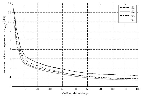
FIGURE 5.37
Dependence of RMSE on the VAR order.

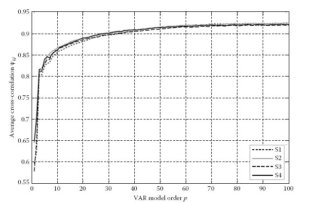
FIGURE 5.38
Dependence of ψ_i,j on the VAR order.

5.3.2.5    Results and Model Validation

Let us first consider the spectrum of a typical measured noise shown in Figure 5.39. It can be observed that it is a typical coloured noise with a high PSD towards the low frequencies. As the frequency increases, the noise PSD decreases. The presence of FM noise PSD is also visible. This noise measurement sample is representative of the statistical noise characteristics detailed in Section 5.2.3.1.

Now we study the PSD of the noise obtained from the VAR(50) simulation. It is clear from Figure 5.40 that the modelled noise successfully captures the coloured nature of the measured noise. The FM noise PSD is also successfully reserved by the model. Although the exact peak-by-peak match is not achieved the measured noise and the modelled noise, the VAR(50) model confidently reflects the overall inverse relationship between the frequency and the noise PSD.

Now we turn to the statistical analysis of the VAR model efficiency. First we consider the frequency domain cross-correlation between the measured noise and its VAR(50) model, as shown in the CDF of Figure 5.41. The CDF represents the dataset of 116 measurements. Figure 5.41 shows that for 90% of the measurements the VAR(50) model achieves a correlation of 0.85–0.98. The typical midrange value of the correlation is around 0.93. These high correlation values suggest that the VAR(50) model efficiently captures and generates the spectral characteristics of the measured noise.

The RMSE ε_rms,f between a given noise measurement and its VAR(50) model ranges from 2 to 7 dB, as shown in Figure 5.42. The typical midrange value of RMSE is around 4.5. We note that for 90% of the cases the RMSE value is below 6 dB, that is, ±3 dB in absolute terms. These statistics affirm that the VAR(50) model successfully regenerates the spectral characteristics of the measured noise.

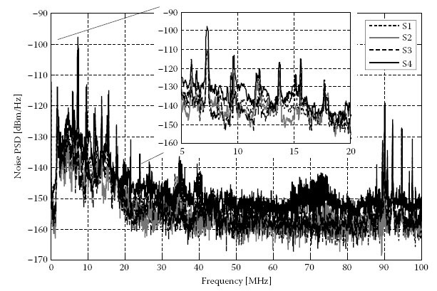
FIGURE 5.39
PSD of a typical measured noise.

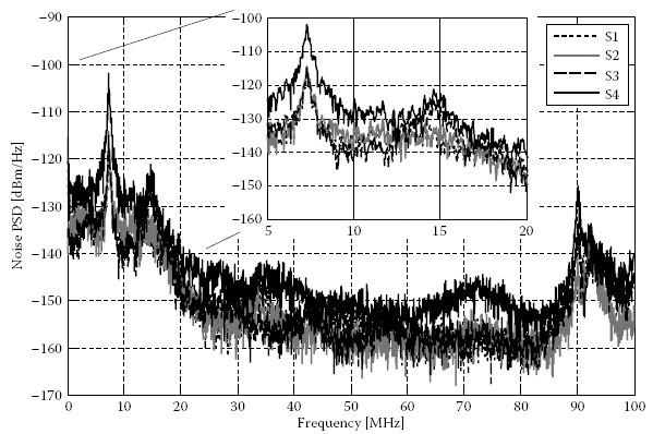
FIGURE 5.40
PSD of the VAR(50) modelled noise corresponding to the measured noise of Figure 5.39.

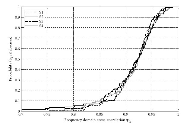
FIGURE 5.41
CDF: Correlation between the spectrum of the measured noise and its VAR(50) model.

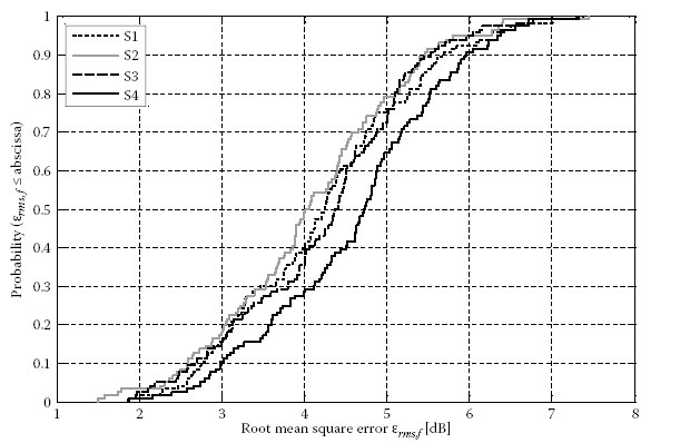
FIGURE 5.42
CDF: RMSE between the spectrum of the measured noise and its VAR(50) model.

5.4    Conclusion

Extensive field measurements recoding MIMO PLC properties in private homes were conducted in seven European countries with an identical measurement set-up according to a harmonised measurement specification. This generated comparable results among all locations and a huge statistical mass of data.

Following highlights were found when interpreting the data:

•  T-style coupler provides less attenuation at the high attenuated channels (important to achieve maximum coverage).

•  CM reception also provides a lower attenuation at the bad links.

•  55 dB is the median attenuation of the main grid in the frequency range 1 MHz < f < 100 MHz, where the attenuation raises with 0.2 dB/MHz.

•  The median attenuation within a private home of any size is 0.11 dB/m² × size (m²) +36.07 dB.

•  The three-phase installations in Germany causes the highest attenuation among the visited European countries.

•  Impedance matching at outlets is quite low, where the star-style coupler shows best and the T-style coupler worst matching properties.

•  Usually the impedance over frequency is identical among the wires at one outlet.

•  Ring wires in the United Kingdom only show minimal lower input impedance than the European continent.

•  The spatial correlation of the MIMO PLC channel is relatively high. For the 2 × 4 MIMO configuration, 60% of the channels and frequencies comprise a spatial correlation of >10 dB, that is, the second spatial stream is >10 dB attenuated compared to the first spatial stream.

•  The background noise is the lowest in the frequency range 30 MHz < f < 87 MHz, where the median PSD is −150 dBm/Hz.

•  The noise level is independent of the size of a home.

•  In the time domain, impulsive noise is present in one-third of the observations, due to the presence of electronic devices like switched mode power supplies or fluorescent lamps.

Furthermore, this chapter presented a new statistical channel model for the MIMO CTF matrix, based on the measurements described. This model allows the generation of random CTFs faithfully reproducing the path loss statistics, multi-path structure and channel correlation coefficients statistically observed within the field data base. Such a model will prove useful to evaluate the performance of existing MIMO PLC transmission systems and to develop new signal processing strategies optimally exploiting the channel characteristics. Modelling of multiple-output noise has been proposed by fitting series of noise measurements to a MTS with a limited set of parameters. This formalism allows reproducing both the noise multi-path structure and the correlation between output ports. In order to improve such studies, it will become important in the future to better understand the noise component of the MIMO PLC channel and to develop stochastic models statistically representative of the variety of noise environments.

Acknowledgements

The authors wish to thank Jose Luis Gonzalez Moreno from Marvell (Spain), Holger Hirsch from the University of Duisburg-Essen (Germany), Hervé Milleret from MStar Semiconductor (France), Andrea Tonello from the University of Udine (Italy) and Nico Weling from Devolo (Germany) for their help in conducting field measurements, in the framework of the ETSI Specialist Task Force (STF) 410. Special thanks goes to Werner Bäschlin from JobAssist (Switzerland) for his excellent support, development and production of the STF 410 couplers which had been used by all teams in the field measurements.

References

1.  R. Hashmat, P. Pagani, A. Zeddam and T. Chonavel, MIMO communications for inhome PLC networks: Measurements and results up to 100 MHz, International Symposium on Power Line Communications and Its Applications (ISPLC), Rio de Janerio, Brazil, 2010.

2.  A. Schwager, Powerline communications: Significant technologies to become ready for integration, PhD dissertation, Universität Duisburg-Essen, Duisburg, Germany, 2010. http://duepublico.uni-duisburg-essen.de/servlets/DerivateServlet/Derivate-24381/Schwager_Andreas_Diss.pdf.

3.  L. Stadelmeier, D. Schneider, D. Schill, A. Schwager and J. Speidel, MIMO for inhome power line communications, International Conference on Source and Channel Coding (SCC), Ulm, Germany, 2008.

4.  Special Task Force 410. http://portal.etsi.org/stfs/ToR/Archive/ToR410v11_PLT_MIMO_measurem.doc.

5.  ETSI TR 101 562-1 V1.3.1, PowerLine Telecommunications (PLT); MIMO PLT; Part 1:Measurement Methods of MIMO PLT.

6.  ETSI TR 101 562–2 V1.2.1, PowerLine Telecommunications (PLT); MIMO PLT; Part 2: Setup and Statistical Results of MIMO PLT EMI Measurements.

7.  ETSI TR 101 562-3 V1.1.1, PowerLine Telecommunications (PLT); MIMO PLT; Part 3: Setup and Statistical Results of MIMO PLT Channel and Noise Measurements.

8.  P. D. Welch, The use of Fast Fourier transform for the estimation of power spectra: A method based on time averaging over short, modified periodograms, IEEE Trans. Audio Electroacoust., 15, 70–73, June 1967.

9.  D. Rende, A. Nayagam, K. Afkhamie, L. Yonge, R. Riva, D. Veronesi, F. Osnato and P. Bisaglia, Noise correlation and its effects on capacity of inhome MIMO power line channels, IEEE International Symposium on Power Line Communications, ISPLC 2011, Udine, Italy, April 2011.

10.   R. Hashmat, P. Pagani, A. Zeddam and T. Chonavel, A channel model for multiple input multiple output inhome powerline networks, IEEE International Symposium on Power Line Communications and Its Applications (ISPLC), Udine, Italy, April 2011.

11.  M. Zimmermann and K. Dostert, A multipath model for the power line channel, IEEE Trans. Commun., 50(4), 553–559, April 2002.

12.  Seventh Framework Programme: Theme 3 ICT-213311 OMEGA, Deliverable D3.2, v.1.2, PLC Channel Characterization and Modelling, February 2011 (http://www.ict-omega.eu/publications/deliverables.html)

13.  A. M. Tonello and F. Versolatto, New results on top-down and bottom-up statistical PLC channel modeling, Third Workshop on Power Line Communications, Udine, Italy, October 2009.

14.  A. M. Tonello, Wideband impulse modulation and receiver algorithms for multiuser power line communications, EURASIP J. Adv. Signal Process., 2007, 1–14.

15.  R. Hashmat, P. Pagani, T. Chonavel and A. Zeddam, A time domain model of background noise for inhome MIMO PLC networks, IEEE Transactions on Power Delivery, 27(4), 2082–2089, October 2012.

16.  A. Neumaier and T. Schneider, Estimation of parameters and eigenmodes of multivariate autoregressive models. ACM Trans. Math. Softwares 2001, 27(1), 27–57.

*  Members to STF 410: Andreas Schwager (STF Leader), Sony, Germany; Werner Bäschlin, JobAssist, Switzerland; Holger Hirsch, University of Duisburg-Essen, Germany; Pascal Pagani, France Telecom, France; Nico Weling, Devolo, Germany; Jose Luis Gonzalez Moreno, Marvell, Spain; Hervé Milleret, Spidcom, France. STF 410 produced following technical reports: [ETSI TR 101 562-1], [ETSI TR 101 562-2] and [ETSI TR 101 562-3].