14

HomePlug AV2: Next-Generation Broadband over Power Line^*

Larry Yonge, Jose Abad, Kaywan Afkhamie, Lorenzo Guerrieri, Srinivas Katar, Hidayat Lioe, Pascal Pagani, Raffaele Riva, Daniel M. Schneider and Andreas Schwager

CONTENTS

14.1  Introduction

14.2  System Architecture

14.2.1  Brief Overview of HomePlug AV

14.2.2  HomePlug AV2 Technology

14.3  PHY Layer Improvements of HomePlug AV2

14.3.1  Multiple-Input Multiple-Output Capabilities with Beamforming

14.3.1.1  MIMO Stream Parser

14.3.1.2  Precoding

14.3.1.3  Beamforming and Quantisation of the Beamforming Matrix

14.3.1.4  Power Allocation

14.3.1.5  Precoding Grouping

14.3.2  Extended Frequency Band up to 86 MHz

14.3.3  Efficient Notching

14.3.3.1  Influence of Windowing on Spectrum and Notch Shape

14.3.3.2  Digital, Adaptive Band-Stop Filters Improve the Notch’s Depth and Slopes

14.3.4  HomePlug AV2 Power Optimisation Techniques

14.3.4.1  Power Back-Off

14.3.4.2  EMC-Friendly Power Boost Using S₁₁ Parameter

14.3.5  Additional PHY Improvements

14.3.5.1  New Time Domain Parameters

14.3.5.2  Additional Constellations

14.3.5.3  Forward Error Correction Coding

14.3.5.4  Line Cycle Synchronisation

14.4  MAC Layer Improvements of HomePlug AV2

14.4.1  Power Save Modes

14.4.2  Short Delimiter and Delayed Acknowledgement

14.4.2.1  Short Delimiter

14.4.2.2  Delayed Acknowledgement

14.4.3  Immediate Repeating

14.5  Gain of HomePlug AV2 Compared to HomePlug AV

14.6  Conclusion

References

14.1  Introduction

The convergence of voice, video and data within a variety of multifunction devices, along with the evolution of high-definition (HD) and 3-dimensional (3D) video, is driving the demand for home connectivity solutions today. Home networks are required to support high-throughput connectivity, guaranteeing at the same time a high level of reliability and coverage (the percentage of links that are able to sustain a given throughput in two nodes or multi-node networks). Applications such as HD television (HDTV), Internet protocol television (IPTV), interactive gaming, whole-home audio, security monitoring and Smart Grid management have to be supported by these new home networks.

During the last decade, in-home power line communication (PLC) has received increasing attention from both the industry and research communities. The ability to reuse existing wires to deploy broadband services is the main attraction of in-home PLC technologies. Another major advantage of PLC is the ubiquity of the power lines that can be used to provide whole-home connectivity solutions. However, as the power line medium had not been originally designed for data communication, the frequency selectivity of the channel and different types of noise (background noise, impulsive noise and narrowband interferers) make power line a very challenging environment, requiring state-of-the-art design solutions.

In 2000, the HomePlug Alliance [1], an industry-led organisation, was formed with the scope of promoting power line networking through the adoption of HomePlug specifications. In 2001, the HomePlug Alliance released the HomePlug 1.0.1 specification and followed up in 2005 with a second release: HomePlug AV. (The letters ‘AV’ stand for ‘audio, video’.) Following its release, HomePlug AV rapidly became the most widespread adopted solution for in-home PLC. To meet the future market needs, in January 2012, the HomePlug Alliance published the HomePlug AV2 specification [2]. HomePlug AV2 enables gigabit-class connection speeds by leveraging the existing power line wires while remaining fully interoperable with other technologies for in-home connectivity, such as HomePlug AV, HomePlug Green PHY [3] (see Chapter 10) and IEEE 1901 [3] (see Chapter 13). The alliance’s AV Technical Working Group (AV TWG) defined new features at both the PHY and MAC layers. These were based on extensive field tests conducted in real-home scenarios across different countries and are included in the HomePlug AV2 specification. The field results obtained by the AV TWG validated HomePlug AV2’s performance claims in terms of both achievable data rate and coverage.

In this chapter, we highlight the key differentiating HomePlug AV2 features as compared with HomePlug AV technology. At the physical (PHY) layer, HomePlug AV2 includes the following:

1.  Multiple-input multiple-output (MIMO) signalling with beamforming to offer the benefit of improved coverage throughout the home, especially on highly attenuated channels. MIMO enables HomePlug AV2 devices to transmit on any two-wire pairs within three-wire configurations comprising line (L), neutral (N) and protective earth (PE) (the coupling is done in the MIMO analogue front-end [AFE] blocks as shown in Figure 14.1).

FIGURE 14.1
HomePlug AV2 Tx and Rx PHY layer. (From HomePlug Alliance, HomePlug AV Specification Version 2.0, HomePlug Alliance, Copyright © January 2012. With permission.)

2.  Extended frequency band up to 86 MHz to increase the throughput especially at the low- to mid-coverage percentages (part of IFFT/FFT [1024; 8192] and mapper blocks as shown in Figure 14.1).

3.  Efficient notching, which allows transmitters to create extremely sharp frequency notches. If electromagnetic compatibility (EMC) regulation will require a fragmented communication spectrum, the throughput loss by excluded frequencies can be minimised (part of power allocation [PA] and window and overlap blocks as shown in Figure 14.1).

4.  Power back-off to increase the HomePlug AV2 data rate while reducing the electromagnetic emissions (part of PA blocks and the AFEs as shown in Figure 14.1).

5.  EMC-friendly power boost to optimise the transmit power by monitoring the input port reflection coefficient (known as the S₁₁ parameter) at the transmitting modem.

6.  Additional PHY Improvements, comprising higher-order quadrature amplitude modulation (4096-QAM) (part of mapper and demodulator blocks as shown in Figure 14.1), higher code rates (8/9 code rate) (part of turbo convolutional decoder as shown in Figure 14.1) and smaller guard intervals (GIs) (part of cyclic prefix blocks as shown in Figure 14.1), to assist in better peak data rates.

At the medium access control (MAC) layer, HomePlug AV2 includes the following:

1.  Power save mode to improve energy efficiency when the device is in standby

2.  Short delimiter to reduce the overhead of the transmission shortening the preamble and frame control (FC) symbols

3.  Delayed acknowledgements to increase the overall transmission efficiency by reducing the interframe spacings

4.  Immediate repeating to expand the coverage by repeating the signal on paths with better signal to noise ratio (SNR) characteristics

All the features listed earlier improve the quality of service (QoS) of AV2 power line modems by improving coverage and robustness of communication links. Moreover, the AV TWG evaluated the performance of the HomePlug AV2 system. The adoption of all these features provides a significant advantage of using HomePlug AV2 versus HomePlug AV.

The following sections provide technical details for all the previously mentioned features. Section 14.2 begins with a brief overview of HomePlug AV technology and then presents the overall HomePlug AV2 system architecture. Sections 14.3 and 14.4 detail the new PHY and MAC layers. Section 14.5 summarises the performance gain of HomePlug AV2 over HomePlug AV. Finally, Section 14.6 concludes this introduction to HomePlug AV2 technology. The Inter System Protocol used by HomePlug AV2 to manage coexistence with other in-home technologies is described in details in Chapter 10.

14.2  System Architecture

14.2.1  Brief Overview of HomePlug AV

HomePlug AV employs PHY and MAC technologies that provide a 200 Mbps-class power line networking capability. The PHY operates in the frequency range of 2–28 MHz and uses windowed orthogonal frequency division multiplexing (OFDM) and a powerful turbo convolutional code (TCC) that provides robust performance within 0.5 dB of Shannon’s limit. Windowed OFDM provides more than 30 dB spectrum notching. OFDM symbols with 917 usable carriers (tones) are used in conjunction with a flexible GI. Modulation densities from BPSK to 1024 QAM are adaptively applied to each carrier based on the channel characteristic between the transmitter (Tx) and the receiver (Rx).

On the MAC layer, HomePlug AV provides a QoS connection-oriented, contention-free service on a periodic time division multiple access (TDMA) allocation and a connectionless, prioritised contention-based service on a carrier sense multiple access/collision avoidance (CSMA/CA) allocation. The MAC receives MAC service data units (MSDUs) and encapsulates them with a header, optional arrival time stamp (ATS) and a checksum to create a stream of MAC frames. The stream is then divided into 512-octet segments, encrypted and encapsulated into serialised PHY blocks (PBs) and packed as MAC protocol data units (MPDUs) to the PHY unit, which then generates the final PHY protocol data unit (PPDU) to be transmitted onto the power line [5]. The HomePlug AV specification is included as one of the two physical layer protocols defined in the IEEE 1901 standard (see Chapter 13).

HomePlug AV2 significantly enhances the capability mentioned earlier to accommodate a new generation of multimedia applications with gigabit-class performance.

14.2.2  HomePlug AV2 Technology

The HomePlug system is specified for in-home communication via the power line channel. These in-home communications are established with the time division duplexing (TDD) mechanism to allow for symmetric communication between peers, as opposed to the classical access system in ADSL which uses two different downstream and upstream throughputs.

The PHY layer employs an OFDM modulation scheme for better efficiency and adaptability to the channel impairments (such as being frequency selective and suffering from narrowband interference and impulsive noise). The HomePlug AV2 OFDM parameters correspond to a system with 4096 carriers in 100 MHz, but only carriers from 1.8 to 86.13 MHz are supported for communication (3455 carriers). The subcarrier spacing of 24.414 kHz was chosen in the HomePlug AV system according to the power line coherence bandwidth characteristic and is maintained in HomePlug AV2 for interoperability.

More significantly, HomePlug AV2 incorporates MIMO capability (see details in the following sections) to improve throughput and coverage.

A block diagram of the PHY layer is shown in Figure 14.1. The HomePlug AV2 system is capable of supporting two network-operating modes: AV-only mode and hybrid mode (refer to 1.0.1 FC encoder in Figure 14.1). Hybrid mode is used for coexistence with HomePlug 1.0.1 stations. For that purpose, a 1.0.1 FC encoder is included for hybrid modes and an AV2 FC encoder is included for both hybrid and AV-only modes. The AV-only mode is used for communications in networks where only HomePlug AV and HomePlug AV2 stations are involved.

Two OFDM paths are also shown to demonstrate how to implement MIMO capabilities with two transmission ports.

Apart from the hybrid or AV-only FC symbols, the payload data can be sent using adaptive bit loading per carrier or robust modes (ROBO) with fixed quadrature phase shift keying (QPSK) constellation and several copies of data interleaved in both time and frequency.

Looking at the data path details in the block diagram (Figure 14.1), the following can be seen: at the Tx side, the PHY layer receives its inputs from the MAC layer. Three separate processing chains are shown because of the different encoding for HomePlug 1.0.1 FC data, HomePlug AV2 FC data and HomePlug AV2 payload data. AV2 FC data is processed by the AV2 FC encoder, which has a turbo convolutional encoder and FC diversity copier, while the HomePlug AV2 payload data stream passes through a scrambler, a turbo convolutional encoder and an interleaver. The HomePlug 1.0.1 FC data passes through a separate HomePlug 1.0.1 FC encoder.

The outputs of the FC encoders and payload encoder lead into a common MIMO OFDM modulation structure, consisting of the following:

•  A MIMO stream parser (MSP) that provides up to two independent data streams to two transmit paths that include two mappers, a phase shifter that applies a 90° phase shift to one of the two streams (to reduce the coherent addition of the two signals)

•  A MIMO precoder to apply Tx beamforming operations

•  Two inverse fast Fourier transform (IFFT) processors

•  Preamble and cyclic prefix insertion

•  Symbol window and overlap blocks, which eventually feed the AFE module with one or two transmit ports that couple the signal to the power line medium

For potential MIMO coupler configuration, the interested reader may refer to Chapter 1.

At the receiver, an AFE with one, two, three or four (N_R) Rx ports operates with individual automatic gain control (AGC) modules and one or more time-synchronisation modules to feed separate FC and payload data recovery circuits. Rxs plugged into power outlets that are connected to the three wires (L, N and PE) might utilise up to three differential-mode Rx ports and one common-mode (CM) Rx port.

The FC data are recovered by processing the received signals through a 1024-point FFT (for HomePlug 1.0.1 delimiters) and multiple 8192-point FFTs and through separate FC decoders for the HomePlug AV2/HomePlug AV and HomePlug 1.0.1 modes. The payload portion of the sampled time domain waveform, which contains only HomePlug AV2 formatted symbols, is processed through the multiple 8192-point FFT (one for each receive port), a MIMO equaliser that receives N_R signals, performs receive beamforming and recovers the two transmit streams, two demodulators, a demultiplexer to combine the two MIMO streams and a channel de-interleaver followed by a turbo convolutional decoder and a de-scrambler to recover the AV2 payload data.

14.3  PHY Layer Improvements of HomePlug AV2

14.3.1  Multiple-Input Multiple-Output Capabilities with Beamforming

The HomePlug AV2 specification incorporates MIMO capabilities with beamforming, which offers the benefit of improved coverage throughout the home, particularly for hard- to-reach outlets. MIMO technology enables HomePlug AV2 devices to transmit and receive on any two-wire pairs within a three-wire configuration. Figure 14.2 shows a three-wire configuration with L, N and PE, as well as an exemplary schematic coupler design (see also Chapter 1). Whereas HomePlug AV always transmits and receives on line–neutral pair (port 1 in Figure 14.2), HomePlug AV2 modems can transmit and receive signals on other pairs as well. Any two pairs formed by the L, N or PE wires (i.e. L–N, L–PE and N–PE) can be used at the Tx. At the Rx, up to four receive ports may be used (see Figure 14.2). The CM signal – indicated as port 4 in Figure 14.2 – is the voltage difference between the sum of the three wires and the ground.

FIGURE 14.2
MIMO PLC channel: different feeding and receiving options.

The numbers of used transmit ports N_T and used receive ports N_R define the MIMO configuration, which is called N_T × N_R MIMO. For example, using L–N and L–PE to feed and receive signals results in a 2 × 2 MIMO configuration. HomePlug AV2 specification supports MIMO configurations with up to two Tx ports and up to N_R Rx ports.

Some regions and homes with older electrical installations do not have the third wire installed in private buildings. A survey on worldwide PE conductor availability may be found in Chapter 1. In this scenario, HomePlug AV2 automatically switches to single-input single-output (SISO) operating mode. HomePlug AV2 also incorporates selection diversity in SISO mode. The ports used for feeding and receiving might be different from the traditional L–N feeding. If, for example, the path from L–PE to L–N offers better channel characteristics than L–N to L–N, the Tx can choose to use the L–PE port for feeding.

A number of studies have been conducted to investigate and model the properties of MIMO transmission through power line channels [6,7,8,9,10,11,12,13,14,15,16,17,18]. More information about the MIMO PLC channel characteristics and channel modelling may be found in Chapters 1 through 5.

The MIMO PLC channel is described by a N_R × N_T channel matrix for each OFDM subcarrier c:

$H\left(c\right)=\left[\begin{array}{ccc}{h}_{11}\left(c\right)& \cdots & h_{1N_T}\left(c\right)\\ ⋮& \ddots & ⋮\\ h_{N_{R}1}\left(c\right)& \cdots & h_{N_R{N}_T}\left(c\right)\end{array}\right]$

(14.1)

with c belonging to the set of used subcarriers (depending, e.g. on the frequency band and tone mask).

HomePlug AV2 supports one or two streams (see Section 14.3.1.1). As HomePlug AV2 supports MIMO configurations with up to two Tx ports and up to N_R Rx ports, the maximum number of supported streams in AV2 is two. The underlying MIMO streams are obtained by a singular value decomposition (SVD) of the channel matrix [19]:

$H\left(c\right)=U\left(c\right)D\left(c\right)V{\left(c\right)}^H,$

(14.2)

where

V and U are unitary matrices, that is, V⁻¹ = V^H and U⁻¹ = U^H (with ^H the Hermitian operator)

D is a diagonal matrix containing the singular values of H

For details about the MIMO channel matrix and the underlying MIMO streams based on the SVD, refer to Chapter 8.

The decomposition into parallel and independent streams by means of the SVD illustrates the MlMO gain: instead of having one spatial stream in SISO, two independent spatial streams are available in a 2 × N_R MIMO configuration with N_R ≥ 2 on average doubling the SISO capacity [6,17,20]. An analysis of the MIMO PLC channel capacity and throughput investigations can be found in Chapter 9.

14.3.1.1  MIMO Stream Parser

Depending on how many streams are used in the transmission, the payload bits have to be split into different spatial streams. This task is performed by the MIMO stream parser (MSP). The MSP splits the incoming bits into one or two streams based on the MIMO mode of operation and the tone map information (see Figure 14.1). To transmit a single-stream payload with spotbeamforming (see Section 14.3.1.3) or for SISO transmissions, the MSP sends all the data at its input to the first mapper. In this case, the MSP operates as if it had only one output and it was connected to the first mapper (see Figure 14.1). To transmit a two-stream payload with eigenbeamforming (see Section 14.3.1.3), the MSP allocates the bits to the two streams.

14.3.1.2  Precoding

Precoded spatial multiplexing or beamforming was chosen as the MIMO scheme, as it offers the best performance by adapting the transmission in an optimal way to the underlying eigenmodes of the MIMO PLC channel. This performance is achieved in various channel conditions. On the one hand, the full spatial diversity gain is achieved in highly attenuated and correlated channels when each symbol is transmitted via each available MIMO path. On the other hand, a maximum bitrate gain is achieved for channels with low attenuation when all available spatial streams are utilised. Beamforming has also many advantages with respect to Rx design. The most simple detection or equaliser algorithm, which is the zero-forcing (ZF) detection (see Section 14.3.1.3), might be used in the case of beamforming. No performance gain is achieved for more sophisticated detection algorithms such as minimum mean squared error (MMSE) or ordered successive interference cancellation (OSIC) detection algorithms when optimum precoding is applied at the Tx [18]. Beamforming also offers flexibility with respect to the Rx configuration. Only one spatial stream may be activated by the Tx when only one receive port is available, that is, if the outlet is not equipped with the third wire or if a simplified Rx implementation is used that supports only one spatial stream. Since beamforming aims to maximise one MIMO stream, the performance loss of not utilising the second stream is relatively small compared to the spatial multiplexing schemes without precoding. This is especially true for highly attenuated and correlated channels, where the second MIMO stream carries only a small amount of information. These channels are most critical for PLC, and adequate MIMO schemes are important. A comparison and analysis of different MIMO schemes may be found in Refs. [18,20,21] and in Chapters 8 and 9.

Beamforming requires knowledge about the channel state information at the Tx to apply the optimum precoding. Usually, only the Rx has channel state information, that is, by channel estimation. Thus, the information about the precoding has to be fed back from the Rx to the Tx. The HomePlug AV2 specification supports adaptive modulation [22,23]. The application of adaptive modulation also requires feedback about the constellation of each subcarrier (tone map); that is, the feedback path is required. The information about the tone maps and the precoding are updated simultaneously upon a change in the PLC channel (realised by a channel estimation indication message). The information about the precoding is quantised very efficiently, and the amount required for the precoding information is in the same order of magnitude as the information about the tone maps. Thus, the overhead in terms of management messages and required memory can be kept low.

The optimal linear precoding matrix F for a precoded spatial multiplexing system can be factored into the two matrices V and P [24]:

$F=VP.$

(14.3)

Note that the subcarrier index is omitted in Equation 14.3 and in the following section to simplify the notation and to allow better legibility. However, it has to be kept in mind that the following vector and matrix operations are applied to each subcarrier separately if not stated otherwise.

P is a diagonal matrix that describes the PA of the total transmit power to each of the transmit streams. PA is considered in more detail in Section 14.3.1.4. V is the right-hand unitary matrix of the SVD of the channel matrix (see Equation 14.2). Precoding by the unitary matrix V is often referred to as unitary precoding or eigenbeamforming.

Figure 14.3 shows the basic MIMO blocks of the Tx. The mappers of the two streams follow the MSP (see Figure 14.1). The two symbols of the two streams are then weighted by the PA coefficients and multiplied by the matrix V (the computation of V is explained in Section 14.3.1.3 in more detail). Finally, each stream is OFDM-modulated separately.

FIGURE 14.3
Precoding at the Tx. (From HomePlug Alliance, HomePlug AV Specification Version 2.0, HomePlug Alliance, Copyright © January 2012. With permission.)

FIGURE 14.4
Performance comparison between SISO, MIMO 2 × 4 spatial multiplexing without precoding (SMX: ZF) and different modes of beamforming, transmit power to noise power of 65 dB, frequency range up to 30 MHz, adaptive modulation using constellations up to 4096-QAM at target BER of 10⁻³ (no error coding).

Figure 14.4 shows the complementary cumulative distribution function (C-CDF) or coverage of the bitrate for SISO and several MIMO modes of operation, over the (1–30 MHz) frequency band. The shown MIMO schemes include spatial multiplexing without precoding (SMX: ZF) [19], different modes of beamforming and, as an additional reference, the Alamouti scheme – a simple but effective space–time code for two transmit ports [Alamouti 1998]. The results of different PA schemes (labelled by mercury water filling [MWF] and simplified PA in the figure) will be discussed later. The MIMO PLC channels used for this analysis (338 channels in total) were obtained during the ETSI STF410 measurement campaign [13,14,15]. At the high coverage point in Figure 14.4 (C-CDF values near 1), the spatial multiplexing without precoding and ZF detection shows no performance improvement compared to SISO. The best performance is achieved by beamforming and the Alamouti scheme. Both schemes exploit the full spatial diversity which is essential to obtain good performance in highly attenuated and correlated channels as shown at the high coverage point here. At a low coverage point (as C-CDF values approach 0) – which comprises good channels with low attenuation – the spatial multiplexing without precoding approaches the performance level of beamforming. The Alamouti scheme in this case approaches the SISO performance, since Alamouti transmits replicas of each symbol and therefore does not achieve a multiplexing gain by utilising the two streams. The spatial multiplexing scheme utilises two streams and thus achieves twice the bitrate performance as compared to SISO and the Alamouti. Overall, beamforming offers the best bitrate for all channel conditions.

14.3.1.3  Beamforming and Quantisation of the Beamforming Matrix

The precoding matrix V is derived by means of the SVD (see Equation 14.2) from the channel matrix H.

There are two possible modes of operation. If only one spatial stream is utilised, single-stream beamforming (or spotbeamforming) is applied. In this case, the precoding is described by the first column vector of V, that is, the precoding simplifies to a column vector multiplication. Note that despite the fact that only one spatial stream is used, both transmit ports are active as the precoding vector splits the signal to two transmit ports. If both spatial streams are used, two-stream beamforming (or eigenbeamforming) is used and the full precoding matrix V is applied in the MIMO precoding block (see Figure 14.3).

Since the information about the precoding matrix has to be fed back from the Rx to the Tx, an adequate quantisation is required. To achieve this goal, the special properties of V are utilised.

The unitary property of V consequences that the columns v_i (i = 1, 2) of V are ortho-normal, that is, the column vectors are orthogonal and the norm of each column vector is equal to 1 [26]. There is more than one unique solution to the SVD: the column vectors of V are phase invariant, that is, multiplying each column vector of V by an arbitrary phase rotation results in another valid precoding matrix.

These properties allow us to represent the complex 2 × 2 matrix V by only the two angles θ and ψ

$V=\left[v_1{v}_2\right]=\left[\begin{array}{cc}{v}_{11}& v_{12}\\ v_{21}& v_{22}\end{array}\right]=\left[\begin{array}{cc}\cos \text{ψ}& \sin \text{ψ}\\ -e^{j\text{θ}}\sin \text{ψ}& e^{j\text{θ}}\cos \text{ψ}\end{array}\right],$

(14.4)

where the range of θ and ψ to represent all possible beamforming matrices is $0\le \text{ψ}\le \text{π}/2$ and $-\text{π}\le \text{θ}\le \text{π}\text{.}$.

According to the phase-invariance property, the first entry of each column (v₁₁, v₁₂) may be set to be real without loss of generality, as defined in Equation 14.4. It is easy to prove that the properties of the unitary precoding matrix are fulfilled. The norm of the column vectors is one: ${\left|v_{11}\right|}^2+{\left|v_{21}\right|}^2={\left|v_{12}\right|}^2+{\left|v_{22}\right|}^2={\sin }^2\left(\text{ψ}\right)+{\cos }^2\left(\text{ψ}\right)=1$. Also, the two columns are orthogonal:

$v_1^H{v}_2=\sin \left(\text{ψ}\right)\cos \left(\text{ψ}\right)-\sin \left(\text{ψ}\right)\cos \left(\text{ψ}\right)e^{-j\text{θ}}{e}^{j\text{θ}}=0.$

(14.5)

In both modes, spotbeamforming and eigenbeamforming, the beamforming vector or beamforming matrix, respectively, is described by both angles θ and ψ. Thus, the signalling of θ and ψ is the same in both modes.

If the MIMO equaliser is based on ZF detection, the detection matrix

$W=H^p={\left(H^{H}H\right)}^{-1}{H}^H$

(14.6)

is the pseudoinverse H^p of the channel matrix H. In case of eigenbeamforming with the precoding matrix V, H can be replaced by the equivalent channel HV in Equation 14.6, and the detection matrix can be expressed by

$W=V^H{H}^p=D^{-1}{U}^H.$

(14.7)

The SNR of the MIMO streams after detection is calculated as

${\text{SNR}}_1=\text{ρ}\frac{1}{{\Vert w_1\Vert }^2}{\text{\hspace{0.17em}\hspace{0.17em}\hspace{0.17em}and\hspace{0.17em}\hspace{0.17em}SNR}}_2=\text{ρ}\frac{1}{{\Vert w_2\Vert }^2}$

(14.8)

with ρ being the ratio of transmit power to noise power and $\Vert w_i\Vert$ the norm of the ith row of the detection matrix W.

Figure 14.5a shows the SNR of the first stream of a MIMO PLC channel. The median attenuation of this link is 40 dB. The ratio of the transmit power to noise power is ρ = 65 dB. The dashed line represents the SNR of spatial multiplexing without precoding and the solid line represents the eigenbeamforming. The SNR of the second stream is displayed in Figure 14.5b.

The two markers X in Figure 14.5a mark a frequency (13 MHz) where good beamforming conditions are found. Different precoding matrices influence the SNR of the two MIMO streams according to Equations 14.6 and 14.8.

Figure 14.5c and d shows the level of the gain or signal elimination due to beamforming for the frequency marked by X in Figure 14.5a and b. The curves in Figure 14.5c and d indicate the SNR. Depending on the precoding matrix, the SNR varies between 6 and 35 dB. No beamforming (ψ = 0 and θ = 0) would result in an SNR of 11 dB. As seen in Figure 14.5c, there is one SNR maximum in the area spanned by ψ and θ. As both streams are orthogonal, one shows an SNR minimum at the location where the other one shows its maximum. The SNR plot in Figure 14.5c and d is 2π periodic in θ, where the black horizontal lines indicate θ = ±π.

The beamforming matrix is quantised efficiently to reduce the amount of feedback required to signal V. A total of 12 bit is used to describe the precoding matrix V. A normal distribution of the real and imaginary part of the entries of the channel matrix H results in a uniform distribution of V. This results in a uniform distribution of θ and a normal distribution of ψ. Optimal performance is achieved by quantifying θ with 7 bit and ψ with 5 bit. This quantisation is chosen such that the loss of the SNR after detection (refer also to Equations 14.6 and 14.8) is within 0.2 dB compared to the optimum beamforming without quantisation.

14.3.1.4  Power Allocation

MIMO PA is applied to two-stream MIMO transmissions. The PA adjusts the power of a carrier on one stream relative to the other stream. For SISO transmissions and MIMO spotbeamforming transmissions, MIMO PA can be bypassed, since there is only one transmit stream. In this case, the only available option is to allocate all the power to the single stream. The PA module is located between the mapper and the precoding block (see Figure 14.1) and performs on the two MIMO streams before eigenbeamforming. The PA in AV2 is designed in a way to not periodically feedback additional information from the Rx to the Tx. The PA evaluates the tone maps of the two streams to set their PA coefficients. It was shown that their performance is very close to the optimal PA (MWF) [27]. PA improves especially highly attenuated channels at the high coverage point.

According to the adaptive modulation, constellation mapping is applied individually for each carrier based on the tone map information for each stream. If the SNR of a carrier on one stream is low enough so that it does not carry any information, the power is allocated to the other stream. The level of power to be assigned is adjustable in 0.5 dB steps.

FIGURE 14.5
Influence of precoding on the SNR: SNR of the first (a) and second (b) stream with and without precoding, transmit power to noise power of ρ = 65 dB, 40 dB average channel attenuation. (From Yonge, L. et al., Hindawi J. Electr. Comput. Eng., 2013, Article ID 892628, Copyright © 2013.) Influence of precoding on the SNR: SNR depending on the precoding matrix at 13 MHz of the first (c) and second (d) stream. (From Yonge, L. et al., Hindawi J. Electr. Comput. Eng., 2013, Article ID 892628, Copyright © 2013.)

Each AV2 Tx selects the level of power adjustment depending on regulatory requirements and its transmit implementation. This level is signalled once to the receive node to be considered at SNR estimation and the generation of the tone map.

14.3.1.5  Precoding Grouping

HomePlug AV2 devices support an expanded frequency spectrum (up to 86.13 MHz; see Section 14.3.2) and one additional stream (utilising MIMO) compared with the 30 MHz for HomePlug AV devices. Thus, HomePlug AV2 devices need to store two tone maps (one for each stream) and one precoding matrix (PCM) per carrier. This significantly increases the memory requirements for an AV2 modem. In order to save memory, HomePlug AV2 devices transmit and store the PCM only on a subset of carriers called precoding pilot carriers (PPCs). At the Tx, the PCMs for the carriers between two adjacent PPCs are obtained via interpolation. The spacing between the PPCs is selected out of a set of predefined values and may be adjusted depending on memory capabilities or channel conditions. The more memory embedded in the modems, the finer the granularity. The performance loss of precoding grouping compared to the quantisation of each subcarrier separately is marginal, due to the high correlation of the precoding matrices of neighboured subcarriers. An investigation about different precoding grouping algorithms for MIMO PLC may be found in [18].

Different classes of AV2 devices may have different memory implementations. Devices where a large memory is embedded may group the carriers with finer granularity. Devices with limited memory have to perform grouping at a coarser granularity. Since the Rx feeds back PCMs, it is important that the Rx is aware of the memory capabilities of the Tx. For instance, a Tx with limited memory will not be able to store and use the PCMs if they are transmitted at a finer granularity from a Rx with large memory. The PCM grouping supported by the Tx is indicated to the Rx via a management message sent by the Tx.

The Rx forwards the PCM for the pilot carriers to the Tx. The Tx reconstructs the pilot PCM information to obtain the precoding matrices for all carriers.

Figure 14.6 shows a reconstruction based upon interpolation in the angle domain (similar to Figure 14.5c and d). The markers labelled by ‘x’ represent the precoding matrix of 17 adjacent subcarriers of a MIMO PLC channel. The markers labelled by the filled circles show the quantised precoding matrices (quantisation with 12 bit per carrier). Some subcarriers use the same precoding matrix, and therefore, the number of circles is less than 17 in Figure 14.6. The linear interpolation with a grouping of eight subcarriers is shown by the unfilled circles in Figure 14.6. The precoding matrices of the interpolated subcarriers resemble the optimal precoding matrix here quite closely.

Figure 14.7 shows the behaviour of the interpolation near notched or masked subcarriers. The location of PPCs may occur in notched bands where the Rx does not have an estimate of the PCM. In such cases, the Rx extrapolates the PCMs on the carriers at the notch edges to get the precoding matrix for the PPC inside the notch. The Rx knows the interpolation applied at the Tx and uses this information to get an extrapolated precoding matrix on PPCs inside a notch.

14.3.2  Extended Frequency Band up to 86 MHz

During the specification development, the AV TWG conducted a measurement campaign, where power line channel and noise measurements were performed in 30 homes located in different European countries as well as in the United States. Such variety was a key ingredient for obtaining insight into the power line at frequencies above those used in HomePlug AV (1.8–30 MHz). Specifically, in every home, all the possible links among at least five different nodes were measured.

FIGURE 14.6
Linear interpolation of the precoding matrix in the angle domain.

FIGURE 14.7
Interpolation of the precoding matrix at the edges of notches. (From HomePlug Alliance, HomePlug AV Specification Version 2.0, HomePlug Alliance, Copyright © January 2012. With permission.)

Examples of channel attenuation and noise PSD are reported in Figures 14.8 and 14.9, respectively.

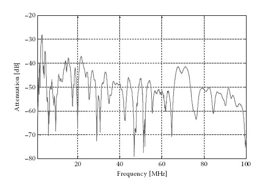
FIGURE 14.8
Example of measured channel transfer function.

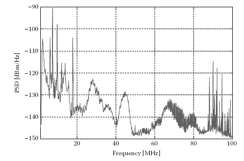
FIGURE 14.9
Example of measured noise PSD.

The final outcome of the analysis was the selection of the 30–86 MHz band. This was based upon the results of the measurement campaign, the present EMC regulations, coverage and complexity targets, as well as the following:

1.  The frequency modulation (FM) band region 87.5–108 MHz must be avoided, as this frequency region presents higher attenuation and higher noise compared to the 30–86 MHz band (see also Figures 14.8 and 14.9). In addition, one can expect that lower transmit power levels will be required in this band in order to protect FM radio services. Therefore, very low operating SNRs could be obtained in this band with negligible coverage increase.

2.  The 30–86 MHz frequency band appears to offer a throughput increase, especially at the low- to mid-coverage percentages; this is due to the fact that while the attenuation is greater compared to the 1.8–30 MHz band, noise is lower. In the past, EMC requirements for the 30–86 MHz frequency band were generally tighter than in the 1.8–30 MHz band. However, regulatory bodies such as CENELEC are currently working towards a stabilisation of the PLC regulation status in Europe (see details on standard FprEN 50561-1 in Chapter 6). Therefore, it can be expected that commonly agreed transmit power masks will be defined soon for the 30–86 MHz frequency range.

3.  Within the HomePlug AV2 specification, it has been possible to provide flexibility in choosing the stop frequency in the 30–86 MHz interval. In particular, an AV2 device implementing a frequency band from 1.8 to X MHz (with 30 < X < 86) will be interoperable with a device implementing a frequency band from 1.8 to Y MHz (with 30 < Y < 86, X ≠ Y).

4.  The 30–86 MHz frequency band extension allows devices to be fully interoperable with the IEEE 1901 devices that use the 1.8–50 MHz frequency band. In fact, HomePlug AV2 devices that implement a frequency band extension shall support the IEEE 1901 bandwidth.

14.3.3  Efficient Notching

HomePlug AV2 increases throughput by allowing devices to minimise the overhead incurred due to EMC notching requirements. While in HomePlug AV the mechanism (‘windowed OFDM’) for creating the PSD notches is fixed and relatively conservative, HomePlug AV2 devices may gain up to 20% in efficiency if they implement additional techniques to accommodate sharper PSD notches. The 20% includes the gain of guard carriers that were excluded by HomePlug AV modems and the reduced transition interval (TI) in the time domain. Such devices gain additional carriers at the band edges and may utilise shorter cyclic extensions, which reduces the duration of the OFDM symbols.

14.3.3.1  Influence of Windowing on Spectrum and Notch Shape

The FFT process uses a rectangular window to cut data out of a continuous stream to convert them from time to frequency domain. The FFT of a rectangular function in the time domain is a sin(x)/x function in the frequency domain. The sin(x)/x becomes 0 at integer multiples of π. Some parts of the signal remain in between the zeros, which results in the unwanted side lobes of an FFT OFDM system. Figure 14.10 shows a sin(x)/x function marked with ‘+’ symbols. Frequency is shown on the horizontal axis. The level of magnitude is shown on the vertical axis, in a logarithmic view.

The process of multiplying a window with an OFDM symbol (see Figure 14.11) in the time domain is aimed to suppress the sharp corners at the beginning and the end of the OFDM symbol in order to obtain smooth transitions. This affects the shape and distances of the side lobes in the frequency domain [29]. There are numerous types of window functions available for implementation such as Hamming, Barlett (triangular), Kaiser, Blackman and Raised Cosine (Hann). A comparison of various window waveforms with the achieved side lobe attenuation is shown in Figure 14.10, which also serves to illustrate the disadvantage of windowing. The side lobes are suppressed, but the main lobe stays wider.

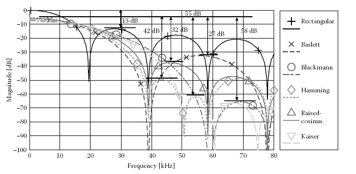
FIGURE 14.10
OFDM side lobes of a single carrier. Comparison of various window functions. (From Yonge, L. et al., Hindawi J. Electr. Comput. Eng., 2013, Article ID 892628, Copyright © 2013.)

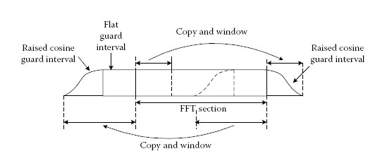
FIGURE 14.11
OFDM symbol with GI and window. (From Yonge, L. et al., Hindawi J. Electr. Comput. Eng., 2013, Article ID 892628, Copyright © 2013.)

The first time the spectrum reaches zero, the distance for all windows is at least twice the frequency of the rectangular window used by the pure FFT. Windowing is considered to be state of the art in signal processing [30].

The process of how a window is applied is shown in Figure 14.11. The original OFDM symbol or the output of the IFFT at the Tx is marked with ‘FFT section’. The GI is copied from the tail samples to the beginning of the symbol. In order to create a window, the symbol has to be expanded further at the beginning and at the end by copying the bits as done for the GI. This expansion is multiplied with the smoothly descending window. The more smoothly the signal approaches zero in the time domain, the lower the side lobes in the frequency domain. This expansion of a symbol is a waste of communication resources, as it does not carry useful information and has to be cut by the Rx.

The two descending slopes in the time domain could overlap, to save communication resources at consecutive OFDM symbols, as shown in Figure 14.12. The new symbol time T_s is measured between the centres of the roll-off intervals (RIs) before and after the symbol. The overlap region is the RI (see Figure 14.12), which is related to the OFDM symbol duration T_s via parameter β

FIGURE 14.12
Consecutive OFDM symbols, GI, RI and windowing. (From HomePlug Alliance, HomePlug AV Specification Version 2.0, HomePlug Alliance, Copyright © January 2012. With permission.)

$RI=\text{β}{T}_{\text{s}}$

(14.9)

and total symbol length T_E

$T_E=\left(1+\text{β}\right)\cdot T_{\text{s}}.$

(14.10)

The HomePlug AV specification allows the usage of several GIs [31,32]. If the shortest GI is selected, HomePlug AV uses a β of RI/(T + GI) = 4.96 μs/(40.96 + 5.56 μs) = 0.1066.

With HomePlug AV2, the TI is introduced. It is relevant for shaping the Tx implementation-dependent windowing, and it does not affect interoperability. The pulse-shaping window and GIs might even be reduced to zero to minimise overhead in the time domain and to efficiently notch. In order to guarantee backward compatibility with previous HomePlug versions, the definition and timings of the parameter RI as shown in Figure 14.12 must stay stable. In contrast to RI, the new parameter TI might be reduced to zero.

There is a balance between these intervals and obtaining a better side lobe attenuation.

Figure 14.13 shows the notch of any OFDM system spectrum that could be obtained by varying the roll-off factors (the β values) of the raised cosine window. Increasing the roll-off factor directly increases the amount of attenuation achieved inside the notches. However, this has the drawback of increased symbol length.

To create notches in the OFDM spectrum, a model is implemented using QAM modulation and notches of omitting a various number of carriers: 1–5 and 10. A max-hold function is implemented in order to create these figures. The 10-carrier notch shows the spectral benefit of windowing. The influence of windowing is hardly visible up to the point of the five-carrier notch. At the five-carrier notch, the difference between no window and the highest simulated β is around 5 dB. The trade-off for this β is an 11% longer symbol time. At the 10-carrier notch, the centre frequency is suppressed by around 15 dB without windowing and almost 30 dB if the HomePlug AV window is applied.

The additional overhead in the time domain is extremely large compared to the improved notch depth. Windowing with a small roll-off factor is sufficient in order to suppress the side lobes outside the used spectrum, but is not recommended to increase the depth of a single carrier notch.

FIGURE 14.13
OFDM spectra with different notch widths and depths achieved with different roll-off.

In the case of the HomePlug AV specification using a β of 0.1066, some guard carriers on the left and right side of a protected frequency range have to be omitted to guarantee the depth of the notch. The North American Carrier Mask requests 10 notches in between 1.7 and 30 MHz. The first carriers as well the last carriers of this spectrum are notched. These two notches have only one slope to the carriers allocated for communications. All other notches have 2 slopes, resulting in a total of 18 notch slopes. The spectrum loses almost 6% of communication resources in the frequency domain. Additionally, the β causes almost 11% of wasted resources in the time domain. Assuming an ideal implementation with maximal sharpness in time as well as frequency domain, it would be possible to regain these communication resources when applying the North American Carrier Mask. If the frequency spectrum becomes more fragmented because of additional notches like those requested by the newly upcoming European regulations [33], these losses will become even more obvious.

14.3.3.2  Digital, Adaptive Band-Stop Filters Improve the Notch’s Depth and Slopes

Although an ideal implementation as described earlier is not possible, digital band-stop filters increase the sharpness of the notches as well as the implementation efforts in hardware. Shrinking the semiconductor manufacturing process to smaller structures, allowing integration of additional functions on the same die size, shifts the balance towards hardware implementation efforts.

The HomePlug AV2 specification gives maximum freedom to the chip implementer. The filter algorithm, order and structure are implementation dependent. An example is documented in [34]. The more efforts placed in the filtering processing, the better the sharpness of the notch slopes. This in turn leads to shorter GI lengths, and thus, more resources are made available for communication. A reduction of the GI down to zero (see Section 14.3.5.1) is possible at short PLC channels without multipath reflections or intersymbol interference.

14.3.4  HomePlug AV2 Power Optimisation Techniques

The HomePlug AV2 standard introduces two novel techniques that can be used to optimise the use of transmit power. The first one, ‘transmit power back-off’, is a technique that reduces the transmitted power spectral density (PSD) for a selected set of carriers when this can be done without adversely affecting performance. Conversely, the second, ‘EMC-friendly power boost’ is a technique that allows the Tx to increase the power on some carriers with the knowledge that this can be done without exceeding regulatory limits.

14.3.4.1  Power Back-Off

In PLCs, the transmit power limit is typically defined as a PSD mask applicable over the range of frequencies used in the standard. And since power line modems are directly connected to the electrical wiring, they are traditionally designed to transmit with the maximum allowed transmit PSD on each frequency (i.e. they do not need to be sensitive to a limited battery supply). In many cases, maximising transmit power leads to the best performance; however, certain definitions of PSD masks combined with certain channel conditions can produce cases where modems can benefit from transmitting at less than the maximum allowed power level.

We illustrate the benefits of transmit power control using the North American regulatory limits as an example. FCC regulations that are applicable to power line devices in North America are commonly interpreted to allow a transmit PSD of −50 dBm/Hz from 1.8 to 30 MHz and −80 dBm/Hz from 30 up to 86 MHz. More details about regulatory limits can be found in Chapter 6. This 30 dB drop in the PSD (at 30 MHz) causes the signal from the higher frequency carriers (above 30 MHz) to have much smaller amplitude than the signal for the low-band carriers (up to 30 MHz). Consequently, when the overall signal is represented in a quantised digital domain, the high-band signal has lower resolution than the signal in the lower band and will therefore also have a limited SNR. This will be evident at the Tx where the 30 dB drop will result in a reduction of 5 bit of resolution for the high-band signal. If the transmit power is backed off in the low band so that the PSD drop is reduced, then the high-band signal will be represented with an increased number of bits of resolution and enjoy increased SNRs out of the Tx.

Another limiting factor is the limited dynamic range of the analogue to digital converter (ADC). We illustrate its impact once again using the example of the North American PSD limits. For the sake of simplicity, we assume a flat power line channel and flat noise spectrum in Figure 14.14. For convenience, the power line channel (curves labelled Rx signal: the transmitted signal after channel attenuation) and noise (curves labelled Rx noise) contributions to the received signal are shown separately. Moreover, the different signals are shown before (dashed line curves) and after (continuous line curves) the analogue amplifier. On the left side of Figure 14.14, the scenario without power back-off is shown: the transmitted signal is 30 dB greater in the 1.8–30 MHz band compared to the 30–86 MHz band. The analogue amplifier brings the received signal to a Level A tailored to optimise the ADC conversion. Since the dominating noise is the ADC noise (black curve), after the ADC converter SNRs of 35 and 5 dB are found below and above 30 MHz, respectively. On the right side of Figure 14.14, the scenario with power back-off is shown: the transmitted signal is reduced by 10 dB in the 1.8–30 MHz frequency band so that it is only 20 dB greater compared to the 1.8–86 MHz band. Again, the analogue amplifier brings the received signal to Level A. However, in this case, the dominating noise is no longer the ADC noise, and the obtained SNRs are 30 and 10 dB in the 1.8–30 and 30–86 MHz, respectively.

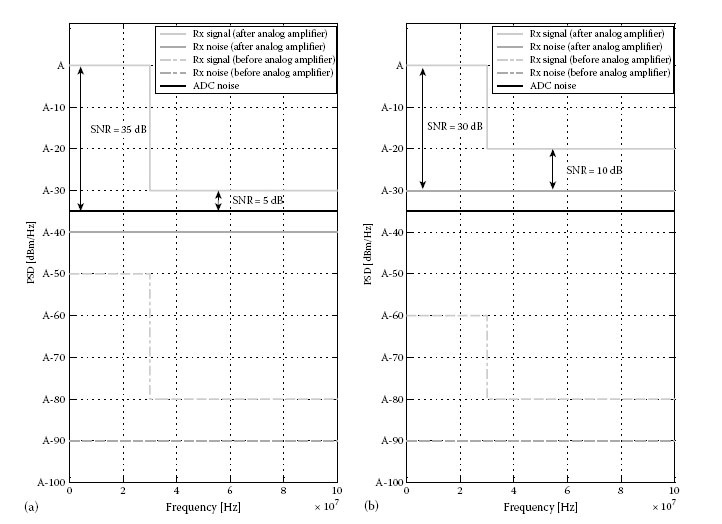
FIGURE 14.14
Benefits of power back-off. (a) No power back-off and (b) 10 dB power back-off. (From Yonge, L. et al., Hindawi J. Electr. Comput. Eng., 2013, Article ID 892628, Copyright © 2013.)

In this example, the power back-off technique results in a 5 dB SNR reduction for the carriers in the lower frequency band and a 5 dB SNR increase for the carriers in the upper frequency band. Given the larger bandwidth of the upper frequency band, there will be an overall throughput gain due to transmit power back-off.

Transmit power back-off is also an effective interference mitigation technique. For instance, in Europe, the ability of a PLC Tx to reduce the transmit power depending on the attenuation link is a possible requirement considered in [33], though the procedure described in CENELEC [33] does not consider QoS requirements of PLC modems.

14.3.4.2  EMC-Friendly Power Boost Using S₁₁ Parameter

The EMC-friendly power boost is a mechanism introduced in the HomePlug AV2 specification to optimise the transmit power by monitoring the input port reflection coefficient at the transmitting modem. This coefficient is known as the S₁₁ parameter. PSD limits as proposed in the HomePlug AV2 specification are based on representative statistics of the impedance match at the interface between the device port and the power line network. In practice, the input impedance of the power line network is frequency selective and varies for different network configurations. This leads to part of the transmit power being dissipated within the Tx. The input port reflection coefficient, or input return loss, is characterised by the S-parameter S₁₁, and the part of transmit power dissipated at the Tx is given by the amount 20 ⋅ log₁₀$\left(\left|{\text{S}}_{11}\right|\right)$ in dB. In situations where the impedance mismatch is large (and thus the S₁₁ parameter is large), only a small part of the input power is effectively transferred to the power lines. In those cases, the electromagnetic interference (EMI) induced by the PLC modem is reduced and can be much lower than the values recommended by EMC regulation limits.

In order to compensate for the frequency-selective impedance mismatch at the interface between the device port and the power line network, HomePlug AV2 modems adapt their transmission mask upon measurement of the S₁₁ parameter at the Tx. The transmitted signal power is increased by an impedance mismatch compensation (IMC) factor, which leads to a more effective power transmission to the power line medium. While increasing the Tx power leads to an increase of the radiated EMI, the design of the IMC factor ensures that the resulting EMI continuously falls below the targeted EMC regulation limits.

A statistical analysis was conducted by the HomePlug Technical Working Group on the practical values of the S₁₁ parameter and the effectiveness of the EMC-friendly power boost technique, based on a series of measurements performed by the ETSI Specialist Task Force 410 [13,14,15,16,17,35]. S₁₁ parameter and EMI measurements were taken over the 1–100 MHz range in six countries: Germany, Switzerland, Belgium, the United Kingdom, France and Spain. The modem used for measurements is described in [13].

The S₁₁ measurements considered in this study consist of three differential feeding possibilities (L–N, N–PE and PE–L) and one CM feeding. For the EMI measurements, we consider the measurements taken with different feeding possibilities, that is, differential feeding, with the other differential ports being unterminated or terminated with 50 O, and CM feeding.

The measurement set used in this analysis consists of 478 frequency sweeps that can be categorised as follows:

1.  Six different locations in Germany and three different locations in France

2.  264 measurements outdoors at 10 m, 43 measurements outdoors at 3 m and 171 measurements indoors

Statistical analysis of this experimental data allowed us to design the practical implementation of the EMC-friendly power boost technique. In the following, we define the IMC factor as (in dB)

$IMC\left(k\right)=\min \left(\max \left(10\cdot {\log }_{10}\left(\frac{1}{1-{\left|{\text{S}}_{11}\left(k\right)\right|}^2}\right)-M\left(k\right),0\right),IM{C}_{\max }\right),$

(14.11)

where

S₁₁(k) is the carrier-dependent estimate of the S₁₁ parameter

M is a margin accounting for possible estimate uncertainties in the measurement of parameter S₁₁

IMC_max is the maximum allowed value of the IMC factor in dB

FIGURE 14.15
CDF of S₁₁ parameter. (From Yonge, L. et al., Hindawi J. Electr. Comput. Eng., 2013, Article ID 892628, Copyright © 2013.)

Figure 14.15 represents the statistical CDF of the S₁₁ parameter as well as the corresponding IMC₀ factor, computed with a margin M of 0 dB. These statistics are based on the experimental data collected during the ETSI STF 410 measurement campaign.

In Figure 14.15, one can read that the S₁₁ parameter is larger than −10 dB in 80% of the cases. This means that for 80% of the records, more than 10% of the energy is reflected back towards the Tx.

More interestingly, Figure 14.16 gives an idea of the potential power increase offered by the EMC-friendly power boost technique:

1.  For 40% of the records, the Tx power could be increased by more than 2 dB to compensate for the impedance mismatch.

2.  For 10% of the records, the Tx power could be increased by more than 4 dB to compensate for the impedance mismatch.

FIGURE 14.16
CDF of IMC parameter. (From Yonge, L. et al., Hindawi J. Electr. Comput. Eng., 2013, Article ID 892628, Copyright © 2013.)

FIGURE 14.17
Difference in dB between the CDFs of the radiated EMI before and after applying the EMC-friendly power boost. (From Yonge, L. et al., Hindawi J. Electr. Comput. Eng., 2013, Article ID 892628, Copyright © 2013.)

We then focused on the effect of the EMC-friendly power boost technique on the radiated EMI statistics. The recorded values allowed the computation of two statistics:

1.  The statistical CDF of the recorded EMI in terms of E-field for all frequencies and feeding possibilities without applying any power boost

2.  The statistical CDF of the recorded EMI in terms of E-field for all frequencies and feeding possibilities when applying the EMC-friendly power boost

Figure 14.17 presents, for each percentile of the CDF, the difference in dB between the E-field CDFs for the two methods of transmission.

Different conclusions can be drawn from this figure. First, the application of the EMC-friendly power boost leads to an increase of the radiated field CDF between 1.2 and 4.8 dB. Note that the extreme value of 4.8 dB arises for one of the lowest values of radiated field and hence is not relevant. Indeed, the lowest values of radiated fields are far from the limits imposed by regulation bodies. Therefore, even with an increase of a few dB, the radiated field will not exceed the limit. Secondly, in general, the application of the EMC-friendly power boost increases the radiated power CDF by about 2 dB. More importantly, the increase of the radiated power CDF is lower than 2 dB for the 25% most radiating cases. This practically means that in the worst-case scenarios where the modems produce the largest EMI, the application of the IMC factor does not increase the EMI by more than 2 dB. This value can be compared with the CDF of the IMC factor given in Figure 14.16. Although the IMC factor is larger than 2 dB in 40% of the cases and larger than 4 dB in 10% of the cases, the application of the EMC-friendly power boost technique does not increase the radiated power CDF extreme values by more than 2 dB. Of course, even an increase of the EMI by 2 dB is not acceptable. Therefore, a margin M of 2 dB is applied when increasing the Tx power using the IMC factor. In practice, this means that the Tx power will be boosted by the value indicated by the IMC factor, minus 2 dB. As a result, even in the most radiating cases, the application of the EMC power boost will not increase the perceived EMI.

Based on this study, we conclude that the application of the EMC-friendly power boost technique provides a significant gain in terms of transmit power increase for a large number of configurations, where the impedance mismatch causes the dissipation of the signal at the Tx. In addition, the statistical analysis shows that this technique will not lead to an increase of the undesirable radiated interference, in particular in the worst EMI scenarios, as long as a margin M of 2 dB is used in the computation of the IMC factor, as specified in Equation 14.11. Finally, a recommended limit for the maximum allowed value of the IMC factor is lMC_max = 6 dB.

14.3.5  Additional PHY Improvements

In addition to the MIMO technology, the frequency band extension, the efficient notching and power optimisation techniques such as the power back-off and the EMC-friendly power boost, other elements of the PHY layer were modified as presented in the following sections.

14.3.5.1  New Time Domain Parameters

In the HomePlug AV2 specification, a number of time domain parameters were refined. As the sampling frequency has increased from 75 to 200 MHz, the number of time samples for a given symbol duration is increased by a factor 8/3. The IFFT interval is 8192 samples in length, and the number of samples in the HomePlug AV GI has increased accordingly. In addition, new features have been added:

1.  The TI defines the part of the RI dedicated to the transition window, allowing more flexibility in the choice of the window (see Section 14.3.3).

2.  A new GI has been defined for the HomePlug AV2 short delimiter (see Section 14.4.2.1).

3.  The payload symbol GI has been made variable and can be as short as 0 μs. It can also be increased up to 19.56 μs. This allows adaptation to a wide range of channel conditions and removes the overhead of the GI for channels that have either very low multipath dispersion or that are completely limited by the receive noise and not by ISI.

14.3.5.2  Additional Constellations

In HomePlug AV, the maximum constellation size is 1024-QAM, corresponding to 10 coded bits per carrier. HomePlug AV2 also provides support for 4096-QAM, which corresponds to 12 bit per carrier. The higher constellation size increases the peak PHY rates by 20%. Practically, the increased throughput will be available mostly on average to very good channels, but even some of the poorer channels sometimes have frequency bands in which high SNRs can be achieved, and thus, the increased constellation size can be used.

14.3.5.3  Forward Error Correction Coding

HomePlug AV2 uses the same duobinary turbo code as HomePlug AV. In addition to the code rates of 1/2 and 16/21, HomePlug AV2 also provides support for a 16/18 code rate. This allows more granularity in the compromise between robustness and throughput degradation. For this new code rate, a new puncturing structure and a new channel interleaver are defined. In addition, a new Physical Block size of 32 octets is defined, which includes specification of a new termination matrix for the forward error correction (FEC) as well as a new interleaver seed table. The 32 octet PBs are used in the PHY level acknowledgements and allow for the acknowledgement of much larger packet sizes that are supported with the increased PHY rates possible in HomePlug AV2.

14.3.5.4  Line Cycle Synchronisation

The HomePlug AV2 specification also describes the device operation in scenarios where there is no alternating current (AC) line cycle (e.g. a direct current [DC] power line) or when the AC line cycle is different from 50 or 60 Hz. In this case, the central coordinator (CCo) is preconfigured to select a beacon period matching either 50 Hz (i. e. beacon period is 40 ms) or 60 Hz (i.e. beacon period is 33.33 ms). One key use case where this feature is useful is the transfer of data towards a multimedia-equipped electrical vehicle during the electrical charging phase (using DC power).

14.4  MAC Layer Improvements of HomePlug AV2

14.4.1  Power Save Modes

HomePlug AV2 stations improve their energy efficiency in standby mode through the adoption of the specific power save mode already defined in the HomePlug Green PHY specification [3] (see Chapter 10 for details). In power save mode, stations reduce their average power consumption by periodically transitioning between awake and sleep states. Stations in the awake state can transmit and receive packets over the power line. In contrast, stations in sleep state temporarily suspend transmission and reception of packets over the power line. We introduce some basic terms useful to describe the power save mode:

1.  Awake window: period of time during which the station is capable of transmitting and receiving frames. The awake window has a range from a few milliseconds to several beacon periods (a beacon period is two times the AC line cycle: 40 ms for a 50 Hz AC line and 33.3 ms for a 60 Hz AC).

2.  Sleep window: period of time during which the station is not capable of transmitting or receiving frames.

3.  Power save period (PSP): interval from the beginning of one awake window to the beginning of the next awake window. PSP is restricted to 2k multiples of beacon periods (i.e. one beacon period, two beacon periods, four beacon periods).

4.  Power save schedule (PSS): the combination of the values of the PSP and of the awake window duration. To communicate with a station in power save mode, other stations in the logical network (AVLN) need to know its PSS.

Potentially, the specification allows aggressive PSSs constituted by an awake window duration of 1.5 ms and a PSP of 1024 beacon period, which will result in over 99% energy savings compared to HomePlug AV. In practice, some in-home applications will require lower latency and response time, and a balance will take place reducing the mentioned gain. This is particularly appealing for applications that foresee a PLC utilisation that is variable during the day (e.g. large utilisation during daytime and small utilisation during nighttime). It is worth highlighting that the HomePlug AV2 specification is flexible in allowing each station in a network to have a different PSS. Given these remarks, in order to enable efficient power save operation without causing difficulties to regular communication, all the stations in a network need to know the PSSs of the other stations. The network CCo has a key role since it grants the requests of the different stations to enter and exit from power save mode operation. Moreover, it distributes the different PSSs to all the stations in the network. When needed, a CCo can

FIGURE 14.18
Example of power save operation in HomePlug AV2 and HPGP. (From HomePlug Alliance, HomePlug GreenPHY, The standard for in-home Smart Grid powerline communications, http://www.homeplug.org, Copyright © 2012.)

1.  Optionally disable power save mode for all stations of the AVLN

2.  Optionally wake up a station in power save mode

The shared knowledge of the PSS allows stations communicating during the common awake windows (the HomePlug AV2 and HPGP specifications have structured the protocols to ensure at least one superposition of all the awake windows occurs). This overlap interval can also be used for transmission of information that needs to be received by all stations within the AVLN.

Figure 14.18 shows an example of PSS of the four stations (A, B, C and D). All stations save more than 75% of energy compared to HomePlug AV. Note that in this example, stations A and B can communicate once every two beacon periods. Moreover, all the stations are always awake at the same time once every four beacon periods, thus preserving communication possibility.

14.4.2  Short Delimiter and Delayed Acknowledgement

The short delimiter and delayed acknowledgement features were added to HomePlug AV2 to improve efficiency by reducing the overhead associated with transmitting payloads over the power line channel. In HomePlug AV, this overhead results in relatively poor efficiency for transmission control protocol (TCP) payloads. One goal that was achieved with these new features was TCP efficiency that improved to be relatively close to that of UDP. In order to send a packet-carrying payload data over a noisy channel, signalling is required for an Rx to detect the beginning of the packet and to estimate the channel so that the payload could be decoded, and additional signalling is needed to acknowledge the payload was received successfully. Interframe spaces are also required between the payload transmission and the acknowledgement for processing time reasons. Indeed, the interframe duration covers the time needed at the Rx to decode the payload, to check accurate reception and to encode the acknowledgement message. This overhead is even more significant for TCP payload, since the TCP acknowledgment payload must be transmitted in the reverse direction.

14.4.2.1  Short Delimiter

The delimiter specified in HomePlug AV contains the preamble and FC symbols and is used for the beginning of data PPDUs as well as for immediate acknowledgements. The length of the HomePlug AV delimiter is 110.5 μs and can represent a significant amount of overhead for each channel access. A new single OFDM symbol delimiter is specified in HomePlug AV2 to reduce the overhead associated with delimiters, by reducing the length to 55.5 μs. Figure 14.19 shows that every fourth carrier in the first OFDM symbol is assigned as a preamble carrier, and the remaining carriers encode the FC. The following OFDM symbols encode data the same as in HomePlug AV.

Figure 14.20 demonstrates the efficiency improvement when the HomePlug AV2 short delimiter is used for the acknowledgement of a CSMA long MPDU, compared to the HomePlug AV delimiter. Not only is the length of the delimiter reduced from 110.5 to 55.5 μs, the response interframe space (RIFS) and contention interframe space (CIFS) can also be reduced to 5 and 10 μs (which is around the fifth part of HomePlug AV’s timing), respectively. Reduction of RIFS requires delayed acknowledgement, which is described in Section 14.4.2.2. Backward compatibility when contending with HomePlug AV devices is maintained by indicating the same length field for virtual carrier sense in both cases, so that the position of the priority resolution symbols (PRS) contention remains the same. A field in the FC of the long MPDU indicates the short delimiter format to a HomePlug AV2 device so that it can correctly determine the length of the payload.

FIGURE 14.19
Short delimiter. (From Yonge, L. et al., Hindawi J. Electr. Comput. Eng., 2013, Article ID 892628, Copyright © 2013.)

FIGURE 14.20
Short delimiter efficiency improvement. (From Yonge, L. et al., Hindawi J. Electr. Comput. Eng., 2013, Article ID 892628, Copyright © 2013.)

14.4.2.2  Delayed Acknowledgement

The processing time to decode the last OFDM symbol and encode the acknowledgement can be quite high, thus requiring a rather large RIFS. In HomePlug AV, since the preamble is a fixed signal, the preamble portions of the acknowledgement can be transmitted while the Rx is still decoding the last OFDM symbol and encoding the payload for the acknowledgement. With the short delimiter, the preamble is encoded in the same OFDM symbol as the FC for the acknowledgement, so the RIFS would need to be larger than for HomePlug AV, eliminating much of the gain the short delimiter provides.

Delayed acknowledgement solves this problem by acknowledging the segments ending in the last OFDM symbol in the acknowledgement transmission of the next PPDU, as shown in Figure 14.21. This permits practical implementation with a very small RIFS, reducing the RIFS overhead close to zero. HomePlug AV2 also allows the option of delaying acknowledgement for segments ending in the second to the last OFDM symbol to provide flexibility for implementers.

14.4.3  Immediate Repeating

HomePlug AV2 supports repeating and routing of traffic not only to handle hidden nodes but also to improve coverage (i. e. performance on the worst channels).

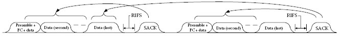
FIGURE 14.21
Delayed acknowledgement. (From Yonge, L. et al., Hindawi J. Electr. Comput. Eng., 2013, Article ID 892628, Copyright © 2013.)

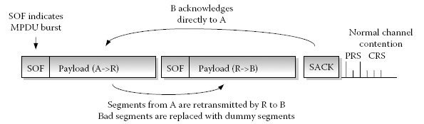
FIGURE 14.22
Immediate repeating channel access for CSMA. (From Yonge, L. et al., Hindawi J. Electr. Comput. Eng., 2013, Article ID 892628, Copyright © 2013.)

With HomePlug AV2, hidden nodes are extremely rare. However, some links may not support the data rate required for some applications, such as a 3D HD video stream. In a network where there are multiple HomePlug AV2 devices, the connection through a repeater typically provides a higher data rate than the direct path for the poorest 5% of channels.

Immediate repeating is a new feature in HomePlug AV2 that enables highly efficient repeating. Immediate repeating provides a mechanism to use a repeater with a single channel access, and the acknowledgement does not involve the repeater. This is shown in Figure 14.22, where station A transmits to repeater R. In the same channel access, repeater R transmits all payload received from station A to station B. B sends an acknowledgement directly to A. With this approach, latency is actually reduced with repeating, assuming the resulting data rate is higher, the obvious criterion for using repeating in the first place. Also, resources required by the repeater are minimised since the repeater uses and immediately frees memory it would require for receiving payload destined for it. Also, there is no retransmission responsibility for failed segments.

14.5  Gain of HomePlug AV2 Compared to HomePlug AV

The AV TWG has evaluated the performance of the HomePlug AV2 specification: this activity was required in order to see if the produced specification would meet the requirements of all stakeholders. The following tables show the performance improvement as compared to HomePlug AV in terms of coverage. These preliminary results are based on a six home field test in Florida, with home sizes 170–300 m². Table 14.1 presents the results in a two-node network scenario: 95% of nodes experienced a throughput improvement greater than 136% compared to HomePlug AV (which means a performance enhancement by a factor of nearly 2.4!). Benefits are even higher when considering the most favourable connections (see the improvement at the 5% coverage value). Table 14.2 considers a four-node scenario where three streams carrying different data are transmitted from one source (e.g. a set-top box) to three different destinations (e.g. TVs). In this case, the greater than 131% improvement in the aggregate throughput is relevant for 99% of networks compared to HomePlug AV.

TABLE 14.1

Improvement of HomePlug AV2 in a 2-Node Network

Coverage Based on UDP Throughput (%)	Percentage of Throughput Improvement of HomePlug AV2 Compared to HomePlug AV (%)
95	>136
5	>220

Source:  Yonge, L. et al., Hindawi J. Electr. Comput. Eng., 2013, Article ID 892628, Copyright © 2013.

TABLE 14.2

Improvement of HomePlug AV2 in a 4-Node Network

Coverage Based on UDP Throughput (%)	Percentage of Throughput Improvement of HomePlug AV2 Compared to HomePlug AV (%)
99	>131
5	>173

Source:  Yonge, L.et al., Hindawi J. Electr. Comput. Eng., 2013, Article ID 892628, Copyright © 2O13.

TABLE 14.3

Maximum PHY Rate Computation

System Configuration (North American Tone Mask)	Max PHY Rate (Mbps)
HomePlug AV (1.8–30 MHz)	197
(917 carriers, 10 bit per carrier, 5.56 μs GI)
IEEE 1901 (1.8–50 MHz)	556
(1974 carriers, 12 bit per carrier, 1.6 μs GI)
HomePlug AV2 SISO (1.8–86.13 MHz)	1012
(3455 carriers, 12 bit per carrier, 0.0 μs GI)
HomePlug AV2 MIMO (1.8–86.13 MHz)	2024
(3455 carriers, 12 bit per carrier, 0.0 μs GI, 2 streams)

Source:  Yonge, L.et al., Hindawi J. Electr. Comput. Eng., 2013, Article ID 892628, Copyright © 2013.

Note that the benefits of the HomePlug AV2 technology are expected to be greater than the ones shown in Tables 14.1 and 14.2 since, for instance, a 2 × 2 MIMO was tested in Florida. A 2 × 3 or 2 × 4 MIMO would likely provide better performance.

Another interesting figure is the theoretical maximum PHY throughput for the system for different options of the standard (Table 14.3). This number represents the throughput of transmitted bits on the PHY layer for optimum channel conditions and gives an idea of the benefits of different features. It can be seen that if the full frequency range is used, HomePlug AV2 provides a 1 Gbps throughput in SISO configuration and 2 Gbps in a MIMO configuration.

14.6  Conclusion

In this chapter, an overview of HomePlug AV2 has been presented. The overall system architecture and the key technical HomePlug AV2 improvements introduced at PHY and MAC layers have been described. It has also been shown that the related performance improvements were achieved by HomePlug AV2 while ensuring backward compatibility with HomePlug AV. In addition, the coexistence with other power line technologies is ensured through the use of the Inter System Protocol (see Chapter 10).

The HomePlug AV2 performance presented in this work has been assessed by AV TWG through simulations based on field measurements.

The results show the significant benefits introduced by the new set of HomePlug AV2 features, both in terms of achievable data rate and coverage.

References

1.  HomePlug Alliance, http://www.homeplug.org, accessed 15 October 2013.

2.  HomePlug Alliance, HomePlug AV Specification Version 2.0, HomePlug Alliance, January 2012.

3.  HomePlug Alliance, HomePlug GreenPHY, The Standard for In-Home Smart Grid Powerline Communications, http://www.homeplug.org, 2010.

4.  IEEE Standard 1901-2010, IEEE standard for broadband over power line networks: Medium access control and physical layer specifications, http://standards.ieee.org/findstds/standard/1901-2010.html (accessed 15 October 2013), 2010.

5.  HomePlug Alliance, HomePlug AV White Paper, http://www.homeplug.org.

6.  R. Hashmat, P. Pagani, A. Zeddam and T. Chonavel, MIMO communications for inhome PLC networks: Measurements and results up to 100 MHz, in Proceedings of the IEEE International Symposium on Power Line Communications and Its Applications (ISPLC’10), Rio de Janeiro, Brazil, March 2010, pp. 120–124.

7.  R. Hashmat, P. Pagani, A. Zeddam and T. Chonavel, A channel model for multiple input multiple output in-home power line networks, in Proceedings of the IEEE International Symposium on Power Line Communications and Its Applications (ISPLC’11), Udine, Italy, April 2011, pp. 35–41.

8.  R. Hashmat, P. Pagani, A. Zeddam and T. Chonavel, Analysis and modeling of background noise for in-home MIMO PLC channels, in Proceedings of the IEEE International Symposium on Power Line Communications and Its Applications (ISPLC’12), Beijing, China, March 2012, pp. 120–124.

9.  R. Hashmat, P. Pagani, T. Chonavel and A. Zeddam, A time domain model of background noise for in-home MIMO PLC networks, IEEE Transactions on Power Delivery, 27(4), 2082–2089, 2012.

10.  D. Rende, A. Nayagam, K. Afkhamie et al., Noise correlation and its effect on capacity of inhome MIMO power line channels, in Proceedings of the IEEE International Symposium on Power Line Communications and Its Applications (ISPLC’11), Udine, Italy, April 2011, pp. 60–65.

11.  D. Veronesi, R. Riva, P. Bisaglia et al., Characterization of in-home MIMO power line channels, in Proceedings of the IEEE International Symposium on Power Line Communications and Its Applications (ISPLC’11), Udine, Italy, April 2011, pp. 42–47.

12.  F. Versolatto and A. M. Tonello, A MIMO PLC random channel generator and capacity analysis, in Proceedings of the IEEE International Symposium on Power Line Communications and Its Applications (ISPLC’11), Udine, Italy, April 2011, pp. 66–77.

13.  ETSI TR 101 562, PowerLine Telecommunications (PLT); MIMO PLT; Part 1: Measurement Methods of MIMO PLT, http://www.etsi.org/deliver/etsi_tr/101500_101599/10156201/01.0_3.01_60/tr_10156201v010301p.pdf (accessed 15 October 2013), 2012.

14.  ETSI TR 101 562, PowerLine Telecommunications (PLT); MIMO PLT; Part 2: Setup and Statistical Results of MIMO PLT EMI Measurements, http://www.etsi.org/deliver/etsi_tr/101500_101599/10156202/01.02.01_60/tr_10156202v010201p.pdf (accessed 15 October 2013), 2012.

15.  ETSI TR 101 562, PowerLine Telecommunications (PLT); MIMO PLT; Part 3: Setup and Statistical Results of MIMO PLT Channel and Noise Measurements, http://www.etsi.org/deliver/etsi_tr/101500_101599/10156203/01.01.01_60/tr_10156203v010101p.pdf (accessed 15 October 2013), 2012.

16.  P. Pagani, R. Hashmat, A. Schwager, D. Schneider and W. Bäschlin, European MIMO PLC field measurements: Noise analysis, in Proceedings of the IEEE International Symposium on Power Line Communications and Its Applications (ISPLC’12), Beijing, China, March 2012.

17.  D. Schneider, A. Schwager, W. Bäschlin and P. Pagani, European MIMO PLC field measurements: Channel analysis, in Proceedings of the IEEE International Symposium on Power Line Communications and Its Applications (ISPLC’12), Beijing, China, March 2012.

18.  Schneider, D., Inhome power line communications using multiple input multiple output principles, Doctoral thesis, University of Stuttgart, Stuttgart, Germany, 2012.

19.  A. Paulraj, R. Nabar and D. Gore, Introduction to Space-Time Wireless Communications, Cambridge University Press, New York, 2003.

20.  L. Stadelmeier, D. Schneider, D. Schill, A. Schwager and J. Speidel, MIMO for Inhome power line communications, in Proceedings of the Seventh International ITG Conference on Source and Channel Coding (SCC’08), Ulm, Germany, January 2008.

21.  A. Canova, N. Benvenuto and P. Bisaglia, Receivers for MIMO PLC channels: Throughput comparison, in Proceedings of the IEEE International Symposium on Power Line Communications and Its Applications (ISPLC’10), Rio de Janeiro, Brazil, March 2010, pp. 114–119.

22.  S. Katar, B. Mashburn, K. Afkhamie, H. Latchman and R. Newman, Channel adaptation based on cyclo-stationary noise characteristics in PLC systems, in Proceedings of the IEEE International Symposium on Power Line Communications and Its Applications (ISPLC’06), Orlando, FL, March 2006, pp. 16–21.

23.  A. M. Tonello, A. Cortés and S. D’Alessandro Optimal time slot design in an OFDM-TDMA system over power-line time-variant channels, in Proceedings of the IEEE International Symposium on Power Line Communications and Its Applications (ISPLC’09), Dresden, Germany, April 2009, pp. 41–46.

24.  A. Scaglione, P. Stoica, S. Barbarossa, G. B. Giannakis and H. Sampath, Optimal designs for space-time linear precoders and decoders, IEEE Transactions on Signal Processing, 50(5), 1051–1064, 2002.

25.  Alamouti, S. M., A simple transmit diversity technique for wireless communications, IEEE Journal on Selected Areas in Communications, 16(8), 1451–1458 1998.

26.  R. A. Horn and C. R. Johnson, Matrix Analysis, Cambridge University Press, New York, 1985.

27.  A. Lozano, A. M. Tulino and S. Verdu, Optimum power allocation for parallel Gaussian channels with arbitrary input distributions, IEEE Transactions on Information Theory, 52(7), 3033–3051, 2006.

28.  L. Yonge, J. Abad, K. Afkhamie, L. Guerrieri, S. Katar, H. Lioe, P. Pagani, R. Riva, D. Schneider, and A. Schwager, An overview of the HomePlug AV2 technology, Hindawi Journal of Electrical and Computer Engineering, 2013, Article ID 892628, 2013.

29.  S. D’Alessandro, A. M. Tonello and L. Lampe, Adaptive pulse-shaped OFDM with application to in-home power line communications, Telecommunications Systems Journal, 51(1), 3–13, 2011.

30.  Harris, F. J., On the use of windows for harmonic analysis with the discrete Fourier transform, Proceedings of the IEEE, 66(1), 51–83, 1978.

31.   K. H. Afkhamie, H. Latchman, L. Yonge, T. Davidson and R. Newman, Joint optimization of transmit pulse shaping, guard interval length, and receiver side narrow-band interference mitigation in the HomePlugAV OFDM system, in Proceedings of the IEEE Sixth Workshop on Signal Processing Advances in Wireless Communications (SPAWC’05), New York, June 2005, pp. 996–1000.

32.  A. M. Tonello, S. D’Alessandro and L. Lampe, Cyclic prefix design and allocation in bit-loaded OFDM over power line communication channels, IEEE Transactions on Communications, 58(11), 3265–3276, 2010.

33.  CENELEC, Power line communication apparatus used in low voltage installations – Radio disturbance characteristics – Limits and methods of measurement – Part 1: Apparatus for in-home use, Final Draft European Standard FprEN 50561-1, June 2011.

34.  Schwager, A., Powerline communications: Significant technologies to become ready for integration, Doctoral thesis, University of Duisburg-Essen, Essen, Germany, 2010.

35.  A. Schwager, W. Bäschlin J. L. Gonzalez Moreno et al., European MIMO PLC field measurements: Overview of the ETSI STF410 campaign & EMI analysis, in Proceedings of the IEEE International Symposium on Power Line Communications and Its Applications (ISPLC’12), Beijing, China, March 2012.

*.  This chapter is adapted and reprinted with permission from Yonge, L. et al., Hindawi J. Electr. Comput. Eng., 2013, Article ID 892628, Copyright © 2013.