8

MIMO PLC Signal Processing Theory

Daniel M. Schneider and Andreas Schwager

CONTENTS

8.1    Introduction

8.2    MIMO Channel Matrix and Its Decomposition in Eigenmodes

8.2.1    MIMO Channel Matrix

8.2.2    Decomposition in Eigenmodes

8.3    MIMO-OFDM System

8.4    Space–Time–Frequency Coding

8.4.1    Alamouti Scheme

8.4.2    General Space–Time–Frequency Codes

8.5    (Precoded) Spatial Multiplexing

8.5.1    Detection

8.5.1.1    Linear Equalisers: Zero-Forcing and Minimum Mean-Squared Error

8.5.1.2    Non-Linear Equalisers: (Ordered) Successive Interference Cancellation and Maximum Likelihood

8.5.2    Eigenbeamforming

8.5.3    Power Allocation for Spatial Multiplexing Streams

8.5.4    Equivalent Channel and Detection

8.5.4.1    Equivalent Channel Including Precoding

8.5.4.2    Whitening Correlated Noise

8.6    Simulation Results

8.7    Conclusions

References

8.1    Introduction

The idea of multiple-input multiple-output (MIMO) [1,2,3] started many research activities, mainly for wireless applications. MIMO technology has recently been successfully introduced by several wireless standards such as IEEE 802.11n, WiMAX and LTE [4]. Compared to their basic single-input single-output (SISO) solutions, they offer a fundamental increase in data rate without the demand of higher transmit power or bandwidth. By using more than two wires, for example, by using the protective earth (PE) wire in addition to the live (L) and neutral (N) wire in in-home power line communications (PLC) (see Chapter 1), the MIMO principles can be applied to PLC as well. The properties of the MIMO PLC channel are discussed in detail in Part I. This chapter deals with the MIMO signal processing theory and the application to MIMO PLC. Before pointing out the outline of this chapter, a brief overview of literature on the application of MIMO schemes to PLC is discussed.

References [5,6,7,8,9] apply space–time codes to access PLC systems and assume perfect isolation between different phase wires. This means that signals fed into one transmit port are only visible at the same receive port. Based on the same channel assumptions [10], proposes an orthogonal frequency division multiplex (OFDM)–based space–time MIMO system for PLC. Reference [11] considers a 2 × 2 MIMO system for in-home applications based on space–frequency-coded multi-tone M-ary frequency shift keying. The wires are assumed to be uncoupled, that is, also no crosstalk between the wires is assumed. Reference [12] considers for the first time a coupled access MIMO PLC channel but also restricts itself to space–time and space–frequency codes. Reference [13] investigates a multiple-input singleoutput (MISO) system for in-home PLC, based on OFDM and space–frequency codes. In JP, two-wire installations are used. However, in the fusion box, three wires are available which make MISO possible if the transmitter is located in the fuse box. The crosstalk between the wires is considered. Reference [14] investigates a MISO access PLC system based on single carrier modulation for narrowband applications. The crosstalk between the wires is considered here as well. The idea of space–time coding is applied to PLC by several authors even if no MIMO channel is assumed. Reference [15] applies space–time codes for coding across OFDM subcarriers to use the diversity across the subcarriers for the frequency-selective PLC channels. Distributed space–time codes are applied in [16] in the context of multi-hop transmission, in which each network node acts as a potential repeater. The use of distributed space–time codes allows an efficient combination at the receiver when different repeater nodes transmit simultaneously. References [17,18,19,20] analyse different MIMO schemes and system proposals for in-home broadband PLC. These algorithms are discussed in the following sections.

The outline of this chapter is as follows. In the first step, the concept of the MIMO channel matrix and its decomposition into parallel and independent MIMO streams based on the singular value decomposition (SVD) is discussed (Section 8.2). Next, this chapter focuses on the comparison of several MIMO schemes and their suitability for broadband PLC, taking into account the characteristics of the MIMO PLC channel.

In order to deal with the frequency-selective characteristic of the PLC channel, today’s SISO-PLC systems use multi-carrier modulation like OFDM. Section 8.3 introduces the basic MIMO-OFDM system including the system assumptions used in this chapter. In the next step, several basic MIMO schemes are introduced and discussed. The different MIMO schemes may be divided into two groups aiming for different goals. MIMO offers spatial diversity to combat fading. The spatial diversity, which is defined by the number of available MIMO paths, is fully exploited by sending the signals over different MIMO paths. These MIMO schemes are called space–time–frequency coded and are introduced in Section 8.4 with the main focus on the Alamouti scheme. Typically, these schemes do not use channel state information (CSI) at the transmitter. The second group of MIMO schemes aims to maximise the throughput by sending different streams via the available transmit ports. These spatial multiplexing (SMX) schemes are discussed in Section 8.5, including precoding at the transmitter where the precoding exploits CSI at the transmitter.

In particular, the signal-to-noise ratio (SNR) after MIMO detection is calculated. The measured MIMO PLC channels obtained during the European measurement campaign (ETSI STF410, see Chapter 5) form the basis of a detailed comparison of the investigated MIMO schemes with respect to the SNR after MIMO detection (see Section 8.6). The basic principles of MIMO signal processing discussed in this chapter form the basis for many of the following chapters in this book dealing with MIMO aspects. The decomposition of the SVD is useful to derive the theoretical channel capacity and the SNR after MIMO decoding and is used to compute the throughput of MIMO PLC systems with adaptive modulation in Chapter 9. This chapter also provides the background knowledge for the MIMO algorithms incorporated in the next-generation broadband PLC specifications (see Chapters 12 and 14).

8.2    MIMO Channel Matrix and Its Decomposition in Eigenmodes

8.2.1    MIMO Channel Matrix

Chapter 1 showed how the PE wire can be used for MIMO communications. The chapter also discussed the coupling of the MIMO signals into the PLC channel. The used input and output ports define the MIMO PLC channel. Figure 8.1a is the schematic measurement set-up with all available MIMO paths. When the delta-style coupler according to Chapter 1 is attached to the MIMO paths, three ports for feeding are available (according to Kirchhoff’s law, up to two might be used simultaneously). The use of the star-style coupler allows up to four receive options. Assume, for example, that the input ports D₁ and D₃ and the output ports S₁, S₂, and S₄ should be used for communication (as indicated by the bold arrows in Figure 8.1a). Then, the resulting MIMO PLC channel is shown in Figure 8.1b with N_T = 2 transmit and N_R = 3 receive ports, resulting in overall six transmission paths.

Figure 8.2 illustrates the magnitude response of the transfer functions of a typical measurement recorded in the ETSI MIMO PLC channel measurement campaign (see Chapter 5) with the delta-style coupler at the transmitter (the ports D₁ and D₃ are used) and the starstyle coupler at the receiver (all four ports S₁–S₄ are used). The frequency range goes up to 100 MHz. Since N_T = 2 transmit and N_R = 4 receive ports are used, overall eight transfer functions are available. The figure aims to illustrate the relationship between the MIMO paths and the same MIMO PLC channel is used in Section 8.2.2 to illustrate the decomposition in eigenmodes. The example shows that the signal, which is fed into one port, is not only visible at the same receive port as the feeding port, but also visible at all the other receive ports. The crosstalk caused by the coupling of the wires results in the presence of all possible MIMO paths. The similar shape of the transfer functions (especially for low frequencies) is due to the same underlying topology of the different MIMO paths. Usually, the wires are run in parallel within the walls facing a similar multi-path propagation. The magnitude responses show the typical frequency-selective behaviour of PLC channels. For details on the MIMO PLC channel properties, refer to Chapters 4 and 5.

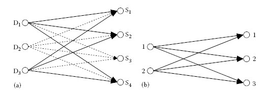
FIGURE 8.1
Constructing the MIMO channel matrix (b) from measured MIMO paths (a) by using the input ports D₁ and D₃ and output ports S₁ S₂ and S₄.

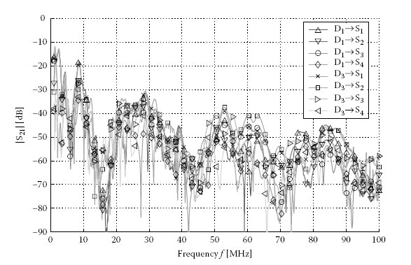
FIGURE 8.2
Magnitude responses of a typical MIMO PLC channel, 0–100 MHz. MIMO configuration: D₁ and D₃ as feeding and S₁−S₄ as receiving ports. SISO configuration: D₁ as feeding and S₁ as receiving port.

With h_ml(f), the complex frequency response of frequency f from feeding port l (l = 1, …, N_T) to receiving port m (m = 1, …, N_R), the MIMO channel matrix of each frequency f is defined as

$H\text{(}f\text{)}=\left[\begin{array}{cccc}{h}_{11}(f)& h_{12}(f)& \cdots & h_{1N_T}(f)\\ h_{21}(f)& h_{22}(f)& \cdots & h_{2N_T}(f)\\ ⋮& ⋮& \ddots & ⋮\\ h_{N_{R}1}(f)& h_{N_{R}2}(f)& \cdots & h_{N_R{N}_T}(f)\end{array}\right]$

(8.1)

Note that h_ml(f) are complex numbers and thus H(f) is a complex matrix. h_ml(f) can be related to the complex transfer function H_ml (n∆f) (n = 1, …, N) as measured by the network analyser (e.g. for N = 1601 measurement points in Chapter 5), that is, the channel is divided into the narrow subchannels measured by the network analyser. For the example shown in Figure 8.1 with the 2 × 3 MIMO set-up, the dimensions of the matrix in Equation 8.1 are 3 × 2. Since the maximum number of feeding and receive ports is N_T = 2 and N_R = 4, up to 2 × 4 MIMO is possible.

8.2.2    Decomposition in Eigenmodes

To simplify the notation and for better legibility, the dependency of f of the channel matrix H(f) will be dropped in the following section. The SVD [21] decomposes the channel matrix H into three matrices:

$H=UD{V}^H.$

(8.2)

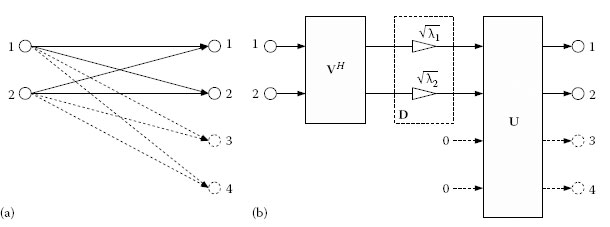
FIGURE 8.3
Decomposition (b) of the MIMO channel (a) into two parallel SISO channels or spatial streams for 2 × 2 MIMO (solid ports and paths) and 2 × 4 MIMO (adding the dashed ports and paths).

D is a diagonal matrix of dimensions R × R containing the real-valued singular values^* ${\sqrt{\text{λ}}}_p,p=1,\dots ,R$ of the channel matrix H:

$D=\text{diag}\left({\sqrt{\text{λ}}}_1,\dots ,{\sqrt{\text{λ}}}_R\right)=\left[\begin{array}{ccc}\sqrt{{\text{λ}}_1}& 0& 0\\ 0& \ddots & 0\\ 0& 0& \sqrt{{\text{λ}}_R}\end{array}\right].$

(8.3)

R is defined as the minimum of the number of transmit and receive ports^† that is, R = min(N_T, N_R). Note that the singular values are real and defined in decreasing order without loss of generality [21]. U and V are unitary matrices, that is, U^-1 = U^H and V^-1 = V^H. (⋅)^H is the Hermitian operator, that is, transpose (⋅)^T and conjugate complex (⋅)^*. (⋅)^-1 is the matrix inverse operator. The dimensions of the complex matrices U and V are N_R × R and N_T × R, respectively. The SVD decomposes the channel matrix into parallel and independent SISO branches or streams [3]. Figure 8.3 visualises the decomposition for N_T = 2 transmit ports and N_R = 2 and N_R = 4 receive ports, respectively. For the example of two transmit ports, at least two receive ports are needed to support R = 2 spatial streams. The full channel matrix in Figure 8.3a (ports drawn with solid lines: 2 × 2 MIMO and including the dashed drawn receive ports: 2 × 4 MIMO) is decomposed into two SISO branches (see Figure 8.3b).

†  R is not necessarily the rank R’ of H,R’ ≤ R. If H has full rank, the rank of H is R’=R. If H does not have full rank R’ < R, some of the singular values ${\sqrt{\text{λ}}}_p,$ are 0.

Since U and V are unitary matrices, multiplication by these matrices preserves the total energy. The singular values ${\sqrt{\text{λ}}}_p$ of D describe the attenuation of the decomposed SISO branches.

Figure 8.4 shows an example of the attenuation of the decomposed MIMO channel. The same channel measurement results are taken as in Figure 8.2. The transmit ports D₁ and D₃ are used as feeding ports and S₁–S₄ as receive ports. The number of transmit ports is N_T = 2 and the number of receive ports is N_R = 4, that is, R = min(N_T, N_R) = 2 singular values ${\sqrt{\text{λ}}}_1$ and ${\sqrt{\text{λ}}}_2$ are obtained. The two singular values are compared to the attenuation of the SISO channel (D₁ is used for feeding and S₁ for receiving). The first stream is less attenuated compared to SISO, while the second stream shows higher and lower attenuation depending on the frequency compared to SISO. The fact that the singular values are in decreasing order results in the first stream being stronger than the second stream. The singular values show the gain of MIMO. Instead of one transmission stream for SISO, two MIMO streams are available. The decomposed streams are still very frequency selective with deep fades. This can be explained by recalling Figure 8.2 around 15 MHz, for example. At this frequency, all MIMO paths experience high attenuation. The singular values of the MIMO channel at this frequency are therefore highly attenuated as well (see frequencies around 15 MHz in Figure 8.4). The attenuation of the singular values not only reflects the attenuation of the MIMO paths but also indicates the spatial correlation between the MIMO paths (see Chapters 4 and 5).

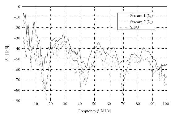
FIGURE 8.4
Comparison of magnitude response between decomposed MIMO streams (singular values) and SISO (same measurement as in Figure 8.2). MIMO configuration: D₁ and D₃ as feeding and S₁−S₄ as receiving ports. SISO configuration: D₁ as feeding and S₁ as receiving port.

8.3    MIMO-OFDM System

The basic MIMO system introduced in this chapter is based on OFDM. OFDM divides the frequency-selective channel into parallel and orthogonal sub-bands or subcarriers [22]. If the number of OFDM subcarriers is large, each sub-band is so narrow that the corresponding magnitude response is flat. Or in other words, the subcarrier spacing must be smaller than the channel coherence bandwidth. The equalisation is simplified and reduced to normalisation by a complex scalar. Each subcarrier is modulated separately which makes OFDM robust against strong fading of certain frequencies or noise in specific sub-bands (narrowband interference). This makes OFDM a suitable modulation scheme for PLC [23]. In order to eliminate intersymbol interference (ISI), OFDM requires a guard interval. Its length depends on the duration of the impulse response. The insertion of the guard interval reduces the bandwidth efficiency of OFDM.

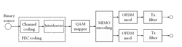
FIGURE 8.5
Block diagram of the MIMO transmitter.

Figure 8.5 shows the basic transmitter structure of the OFDM-based MIMO system with two transmit ports. Typically, the bits of the binary source are encoded by forward error correction (FEC). The FEC is drawn by dashed lines since this chapter focuses on the following blocks and does not consider FEC. The encoded bits are modulated by the quadrature amplitude modulation (QAM) block. The QAM may comprise different modulation orders depending on the subcarrier index (see Section 9.3.1). Next, the complex QAM symbols are processed by the MIMO encoding block. The MIMO encoding may comprise a serial-to-parallel (S/P) conversion to split the symbols to the different transmit ports and may comprise precoding (see Section 8.5). In the case of space–time–frequency coding (see Section 8.4), the symbols are rearranged within this block. The complex symbols of each MIMO stream are OFDM-modulated and the digital time-domain signal is obtained. The block transmitter (Tx) filter comprises impulse shaping, frequency up conversion^*, transmit filtering and digital-to-analogue (D/A) conversion. Finally, the analogue signal is transmitted via the two transmit ports to the MIMO PLC channel.

Figure 8.6 shows the block diagram of the MIMO receiver with four receive ports. The four receiver front-ends (receiver [Rx] filters) receive the signals from the four receive ports and include receive filters, analogue-to-digital (A/D) converters and the frequency down- conversion. Next, each signal is OFDM demodulated. The MIMO processing at the receiver depends on the deployed MIMO scheme and is discussed in detail in the following sections. In case of SMX schemes, the MIMO decoding block contains an equaliser or detection to obtain the two logical MIMO streams and a parallel-to-serial (P/S) conversion to obtain the complex QAM symbols. The QAM symbols are further processed by the QAM demapper. Finally, the demodulated bits are decoded by the FEC decoding to obtain estimates of the transmitted bits.

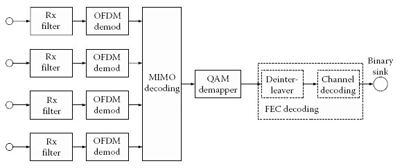
FIGURE 8.6
Block diagram of the MIMO receiver.

The FEC shown in Figures 8.5 and 8.6 illustrates an example containing channel coding and interleaving. However, different architectures are possible, for example, an outer and inner code with several interleavers, turbo codes or low-density parity check (LDPC) codes (see the PLC systems described in Part III of this book).

The MIMO system introduced here works on the level of QAM symbols; the MIMO encoding follows the QAM modulation in the transmitter and precedes QAM demodulation in the receiver. The FEC processes a single bit stream. This coding is often called vertical coding since the streams of the multiple transmit ports are encoded together. On the other hand, horizontal coding handles each MIMO stream separately. Starting from a SISO system, vertical coding allows an easy evolution without changing the encoding and decoding stages. This may be preferable for the further development of a SISO system toward a MIMO communications system to keep the downward compatibility, for example, of a given standard and to reduce complexity.

The receiver in Figure 8.6 does not contain synchronisation or channel estimation. Perfect synchronisation and channel estimation are assumed. Furthermore, this chapter assumes in the following an uncoded system without FEC.

As explained earlier, OFDM decomposes the bandwidth of the channel into small intervals given by multiple subcarriers. In the following, N is the number of subcarriers and n (n = 1, …, N) is the subcarrier index. The channel matrix H(n) of each subcarrier n describes the system between OFDM modulation at the transmitter and OFDM demodulation at the receiver including the couplers. The channel matrix H(n) includes not only the MIMO PLC channel but also includes all filters in the transmitter and receiver. s_k(n) describes the N_T × 1 symbol vector containing the symbols transmitted via the N_T transmit ports and r_k(n) the N_R × 1 received symbol vector of the N_R receive ports after OFDM demodulation of carrier n and time k. The transmit symbols s_l,k(n) (l = 1, …, N_T) have the average power P_T/N_T, where P_T is the total transmit power. The system between the input of the OFDM modulator and the output of the OFDM demodulator is described by

$r_k(n)=H(n)s_k(n)+n_k(n),$

(8.4)

where n_k(n) is the symbol vector containing the noise samples of subcarrier n and time k. The noise samples are assumed to follow a zero mean Gaussian distribution with variance N₀ and are independent for each subcarrier and receive port. The channel is assumed to not change during several OFDM symbols. Typically, the in-home PLC channel experiences long-term time variation, for example, when the network topology changes (toggling of a light switch or a new device is plugged to the mains grid). Additionally, there are short-term and typically line cycle–dependent time variations caused by impedance-modulating devices such as small-sized power supplies. In the following, a quasi-static channel is assumed. Thus, H(n) does not include the time index k. The block diagram of the MIMO-OFDM system is shown in Figure 8.7 for N_T = 2 and N_R = 4.

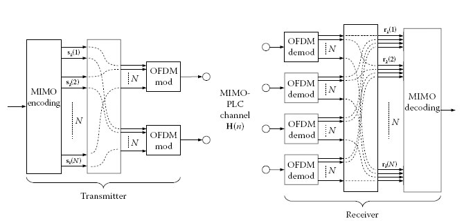
FIGURE 8.7
Block diagram of the MIMO-OFDM system for N_T = 2 and N_R = 4.

8.4    Space–Time–Frequency Coding

The number of available MIMO paths defines the spatial diversity. A MIMO system with N_T transmit ports and N_R receive ports provides the maximal spatial diversity of order N_TN_R. Space–time–frequency codes aim to transmit the signals via each available MIMO path to achieve the full spatial diversity. Space–time block codes achieve this goal by transmitting replicas of each symbol via the different transmit ports at several time instances. The transmission of replicas makes transmission more reliable. However, the bitrate is not maximised. Orthogonal space–time block codes are a subclass of these codes, allowing easy decoding. For the special case of two transmit ports as deployed here for in-home PLC, the orthogonal space–time block codes lead to the well-known Alamouti scheme [24] which is introduced in Section 8.4.1. Several other space–time–frequency codes are discussed briefly in Section 8.4.2.

8.4.1    Alamouti Scheme

The Alamouti scheme encodes two QAM symbols. At the first time instance, k, the two symbols b_1,k(n) and b_2,k(n) are transmitted on subcarrier n via transmit port 1 and 2, respectively, forming the transmit symbol vector $s_k\left(n\right)=\left[\begin{array}{c}{b}_{1,k}\left(n\right)\\ b_{2,k}\left(n\right)\end{array}\right]$. At the second time instance, (k+1), the symbols $-b_{2,k}^{*}\left(n\right)$ and $b_{1,k}^{*}\left(n\right)$ are transmitted via transmit port 1 and 2, respectively. Note that (⋅)^* is the conjugate complex operator. The transmit symbol vector is $s_{k+1}\left(n\right)=\left[\begin{array}{c}-b_{2,k}^{*}\left(n\right)\\ b_{1,k}^{*}\left(n\right)\end{array}\right]$. Two QAM symbols are transmitted during two time instances or OFDM symbols over the two transmit ports. Thus, the spatial code rate is r_S = 1. Each symbol is transmitted via each transmit port and reaches the receiver on every possible MIMO path. Therefore, the full spatial diversity N_TN_R is achieved. The Alamouti scheme works independently of the number of receive ports. MISO is possible as well. Figure 8.8 shows the block diagram of the Alamouti scheme. The space–time encoding is illustrated, using the first subcarrier as an example.

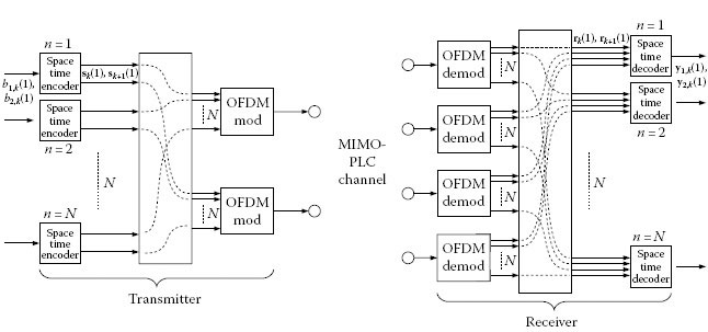
FIGURE 8.8
Block diagram of the MIMO-OFDM Alamouti system, the space–time processing is shown, using the first sub-carrier as an example, N_T = 2 and N_R = 4.

The two transmit symbol vectors are summarised in the space–time coding matrix:

$S(n)=\left[s_k(n)s_{k+1}(n)\right]\text{\hspace{0.17em}=}\left[\begin{array}{cc}{b}_{1,k}(n)& -b_{2,k}{(n)}^{*}\\ b_{2,k}(n)& b_{1,k}{(n)}^{*}\end{array}\right]$

(8.5)

The two columns of S(n) are orthogonal, allowing simple decoding at the receiver. According to Equations 8.4 and 8.5, the received symbol vectors at the two time instances are

$r_k\left(n\right)=H\left(n\right)s_k\left(n\right)+n_k\left(n\right),$

(8.6)

$r_{k+1}\left(n\right)=H\left(n\right)s_{k+1}\left(n\right)+n_{k+1}\left(n\right).$

(8.7)

Note that it is assumed that the channel does not change during the two time instances, that is, H_k(n) = H_{k + 1}(n) = H(n).

Taking the conjugate complex of Equation 8.7 and rearranging the channel matrix

$H\left(n\right)=\left[h_1\left(n\right)h_2\left(n\right)\right]$

(8.8)

with the two column vectors h₁(n) and h₂(n) into a new channel matrix

$\stackrel{\vee }{H}\left(n\right)=\left[\begin{array}{cc}{h}_2^{*}\left(n\right)& -h_1^{*}\left(n\right)\end{array}\right]$

(8.9)

results in

$r_{k+1}^{*}\left(n\right)=\stackrel{\vee }{H}\left(n\right)s_k\left(n\right)+n_{k+1}^{*}\left(n\right).$

(8.10)

Writing Equations 8.6 and 8.10 in matrix notation provides

$\left[\begin{array}{c}{r}_k\left(n\right)\\ r_{k+1}^{*}\left(n\right)\end{array}\right]=\underset{G\left(n\right)}{\underbrace{\left[\begin{array}{c}H\left(n\right)\\ \stackrel{\vee }{H}\left(n\right)\end{array}\right]}}{s}_k\left(n\right)+\left[\begin{array}{c}{n}_k\left(n\right)\\ n_{k+1}^{*}\left(n\right)\end{array}\right],$

(8.11)

where G(n) is the concatenated channel matrix. Since the columns of S(n) are orthogonal, the columns of G(n) are also orthogonal, that is,

$G^H\left(n\right)G\left(n\right)=\text{β}\left(n\right)I_2$

(8.12)

with $\text{β}\left(n\right)={\Vert H\left(n\right)\Vert }_F^2$, where ${\Vert H\left(n\right)\Vert }_F=\sqrt{{\displaystyle {\sum }_{l=1}^{N_T}{\displaystyle {\sum }_{m=1}^{N_R}{\left|h_{ml}\left(n\right)\right|}^2}}}$ is the Frobenius norm of the channel matrix H(n) and h_ml(n) is the matrix element m, l of the channel matrix H(n).

Left multiplying $\frac{1}{\text{β}\left(n\right)}{G}^H\left(n\right)$ on Equation 8.11 yields

$\begin{array}{l}{y}_k\left(n\right)=\left[\begin{array}{c}{y}_{1,k}\left(n\right)\\ y_{2,k}\left(n\right)\end{array}\right]=\frac{1}{\text{β}\left(n\right)}{G}^H\left(n\right)\left[\begin{array}{c}{r}_k\left(n\right)\\ r_{k+1}^{*}\left(n\right)\end{array}\right],\\ =s_k\left(n\right)+\frac{1}{\text{β}\left(n\right)}{G}^H\left(n\right)\left[\begin{array}{c}{n}_k\left(n\right)\\ n_{k+1}^{*}\left(n\right)\end{array}\right],\\ =\left[\begin{array}{c}{b}_{1,k}\left(n\right)\\ b_{2,k}\left(n\right)\end{array}\right]+\frac{1}{\text{β}\left(n\right)}{G}^H\left(n\right)\left[\begin{array}{c}{n}_k\left(n\right)\\ n_{k+1}^{*}\left(n\right)\end{array}\right],\end{array}$

(8.13)

where y_k(n) contains estimates of the transmit symbol vector $s_k\left(n\right)=\left[\begin{array}{c}{b}_{1,k}\left(n\right)\\ b_{2,k}\left(n\right)\end{array}\right]$ which are superimposed with the filtered noise. Equation 8.13 shows the processing by the Alamouti scheme. In a first step, the first received symbol vector r_k(n) and the conjugate complex of the following received symbol vector $r_{k+1}^{*}\left(n\right)$ are stacked into one vector. Next, $\frac{1}{\text{β}\left(n\right)}{G}^H\left(n\right)$ is formed based on the channel matrix H(n). The multiplication of the stacked receive vector by $\frac{1}{\text{β}\left(n\right)}{G}^H\left(n\right)$ leads to estimates of the two transmitted symbols corrupted by noise. Also, according to Equation 8.13, the signal energy of the symbols after Alamouti processing is $E\left\{{\left|b_p\right|}^2\right\}=\frac{P_T}{2}\left(p=1,2\right)$ and the variance of the filtered noise is ${\left[\frac{1}{\text{β}\left(n\right)}{G}^H\left(n\right)\frac{1}{\text{β}\left(n\right)}G\left(n\right)\right]}_{pp}{N}_0=\frac{N_0}{\text{β}\left(n\right)}\left(p=1,2\right)$ with [⋅]_ml the matrix element with position (m, l). Hence, the SNR after Alamouti processing of subcarrier n is calculated as

$\mathrm{\Lambda }\left(n\right)=\frac{\left(\frac{P_T}{2}\right)}{\left(\frac{N_o}{\text{β}\left(n\right)}\right)}={\Vert H\left(n\right)\Vert }_F^2\frac{\text{ρ}}{2}$

(8.14)

with ρ = P_T/N₀. The factor 1/2 results from the distribution of the total transmit power over the two transmit ports. The SNR is the same for both symbols since each symbol is transmitted via each MIMO path. For the same reason, the Alamouti scheme does not benefit from any unequal power allocation (PA) to the two transmit ports.

The Alamouti coding shown here is applied in space and time. A space–frequency coding is possible as well. In this case, the two transmit symbols are not assigned to two time instances but are assigned to two adjacent subcarriers at the same time instant. Correct decoding requires that the channel matrices of the two adjacent subcarriers are identical. This assumption is usually fulfilled for a sufficient large number of subcarriers. However, only small differences in the channel matrices of adjacent subcarriers may lead to distortions. This can cause errors in detection, especially for high QAM constellations, such as 1024-QAM or 4096-QAM.

8.4.2    General Space–Time–Frequency Codes

As explained in the previous subsection, the Alamouti scheme is an orthogonal space–time or space–frequency block code for two transmit ports. There are also orthogonal space–time or space–frequency block codes for more than two transmit ports. In order to keep the orthogonal property for simple decoding, the spatial code rate r_S is decreased compared to two transmit ports with r_S < 1 [25]. Non-orthogonal space–time–frequency block codes achieve higher spatial code rates while still achieving full spatial diversity. Reference [26] proposes a full diversity space–time code for two transmit ports, which achieves a spatial code rate of r_S = 2. This code was further developed in [27] for an arbitrary number of transmit ports. Reference [20] and references therein discuss space–time–frequency block codes for MIMO PLC. For PLC, space–frequency codes are preferred to space–time codes since the quasi-static PLC channel offers no temporal diversity. Note that the Alamouti scheme requires that the channel does not change over two consecutive OFDM symbols. Therefore, no temporal diversity is exploited by the Alamouti scheme; the encoding of the Alamouti scheme is designed to achieve the full spatial diversity. High-rate space–frequency codes require computationally complex maximum likelihood (ML) decoding. In ML decoding, an estimate of the transmitted code word is found by comparing the received code word to all possible code words and finding the most likely one. The complexity increases exponentially with the number of transmit ports and the block length (number of bundled subcarriers) to the basis of the modulation order. The computational complexity may be too high for implementation, especially for high QAM constellations, such as 1024-QAM. Sphere decoding [28] alleviates the burden of ML decoding. However, the application of adaptive modulation is difficult because calculation of the carrier specific SNR after decoding is not possible. Adaptive modulation (see later) already adapts to the frequency fading which makes space–frequency codes less effective for PLC (see also Section 9.3.2).

8.5    (Precoded) Spatial Multiplexing

SMX aims to increase the bitrate by transmitting different streams via the different transmit ports. The number of MIMO streams or spatial code rate r_S is limited by the minimum of transmit and receive ports^*:

$r_{\text{S}}\le \min \left(N_T,N_R\right).$

(8.15)

The spatial diversity depends on the detection algorithm and the application of precoding. Figure 8.9 illustrates the basic block diagram of the OFDM-based SMX system. Two complex QAM symbols are assigned to a vector $b_k\left(n\right)=\left[\begin{array}{c}{b}_{1,k}\left(n\right)\\ b_{2,k}\left(n\right)\end{array}\right]$ for each subcarrier n. F(n) is an optional precoding matrix. If no precoding is considered, F(n) = I_NT and therefore s_k(n) = b_k(n). The received symbol vector r_k(n) is the superposition of both transmitted symbols weighted by the channel matrix H(n) according to Equation 8.4. MIMO detection aims to recover the two transmitted streams. In this figure, linear detection is considered, as described by the detection matrix W(n).

Section 8.5.1 describes different detection algorithms. In a next step, precoding is introduced. The optimum precoding matrix can be separated into unitary precoding (see Section 8.5.2) and PA (see Section 8.5.3). Finally, Section 8.5.4 explains how to combine precoding and an optional noise whitening filter together with the channel matrix to obtain an equivalent channel. This equivalent channel can be used to apply the detection algorithms introduced in Section 8.5.1. For convenience and better legibility, the subcarrier index n and time index k are dropped in the following. However, it has to be kept in mind that the following vector and matrix operations are applied for each subcarrier separately if not stated otherwise.

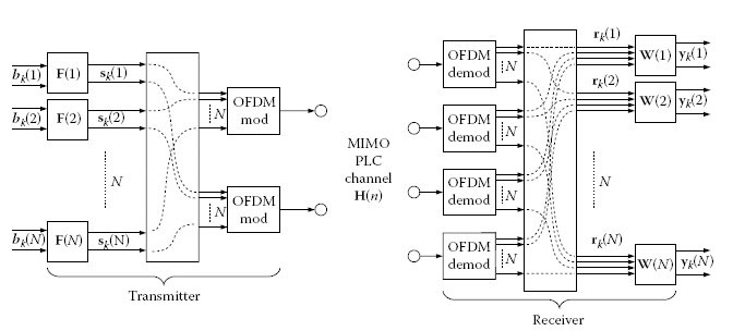
FIGURE 8.9
Block diagram of the MIMO-OFDM spatial multiplexing system with precoding, N_T = 2 and N_R = 4.

8.5.1    Detection

The detection or equaliser algorithms can be separated into linear and non-linear equalisers. In the following, different detection algorithms are briefly introduced. Details may be found, for example, in [3,29].

8.5.1.1    Linear Equalisers: Zero-Forcing and Minimum Mean-Squared Error

Referring to Figure 8.9, the detection matrix W is applied on the received symbol vector r to obtain estimates of the transmit symbol vector s. With r = Hs + n according to Equation 8.4, we obtain

$y=Wr=WHs+Wn.$

(8.16)

Assume that the total transmit power P_T is equally distributed among the N_T transmit ports and that the noise power N₀ is the same on all N_R receive ports. According to Equation 8.16, the pth symbol y_p (pth row of y, p = 1, …, r_S) contains the pth transmit symbol s_p of s. s_p is weighted by the diagonal entry [WH]_pp in Equation 8.16; the signal energy is therefore ${\left|{\left[WH\right]}_{pp}\right|}^2\frac{P_T}{N_T}.y_p$. y_p is also disturbed by the interchannel interference from the other transmit symbols ${\text{s}}_i\left(i=1,\dots ,r_{\text{S}},i\ne p\right)$ which is described by the off-diagonal elements of WH in Equation 8.16. The energy of the interference is then $\frac{P_T}{N_T}{\displaystyle {\sum }_{i=1,i\ne p}^{r_{\text{S}}}{\left|{\left[WH\right]}_{pi}\right|}^2}$. Additionally, y_p is corrupted by noise. The noise variance is given by ${\left[\text{W}{\text{W}}^H\right]}_{pp}{N}_0$. The signal to interference plus noise ratio (SINR) after linear detection of the streams p = 1, …, r_S is then

${\mathrm{\Lambda }}_p=\frac{{\left|{\left[WH\right]}_{pp}\right|}^2\frac{P_T}{N_T}}{{\displaystyle {\sum }_{i=1,i\ne p}^{r_{\text{S}}}{\left|{\left[WH\right]}_{pp}\right|}^2\frac{P_T}{N_T}+{\left[W{W}^H\right]}_{pp}{N}_0}}=\frac{{\left|{\left[WH\right]}_{pp}\right|}^2}{{\displaystyle {\sum }_{i=1,i\ne p}^{r_{\text{S}}}{\left|{\left[WH\right]}_{pi}\right|}^2+{\left[W{W}^H\right]}_{pp}\frac{N_T}{\text{ρ}}}},$

(8.17)

with ρ = P_T/N₀. Note that the interference term ${\displaystyle {\sum }_{i=1,i\ne p}^{r_{\text{S}}}{\left|{\left[WH\right]}_{pi}\right|}^2}$ in Equation 8.17 is equal to 0 if r_S = 1.

Basically, there are two types of linear receivers: zero-forcing (ZF) and minimum mean-squared error (MMSE) detection. ZF detection aims to remove the interchannel interference and does not take the noise into account. MMSE detection minimises both the noise and interchannel interference. The diversity order of the linear SMX receivers is $N_R-N_T+1\left(N_R\ge N_T\right)$ [29].

8.5.1.1.1 Zero-Forcing

The detection matrix W of ZF is the pseudoinverse [⋅]⁺ of the channel matrix H:

$W=W_{\text{ZF}}=H^{+}={\left(H^{H}H\right)}^{-1}{H}^H.$

(8.18)

Applying W = W_ZF according to Equation 8.18 to the received vector r according to Equation 8.4 results in

$\begin{array}{l}y=Wr=W\left(Hs+n\right)=H^{+}Hs+H^{+}n,\\ ={\left(H^{H}H\right)}^{-1}{H}^{H}Hs+H^{+}n=s+H^{+}n.\end{array}$

(8.19)

Equation 8.19 shows again the design criterion. If the noise is zero, the transmit symbol vector is recovered and the interchannel interference is removed completely. However, if there is noise, the variance of H⁺n after detection might be increased compared to the variance of n.

Replacing Equation 8.18 in Equation 8.17 results in the SINR after detection

${\mathrm{\Lambda }}_p=\frac{1}{{\left[W{W}^H\right]}_{pp}}\frac{\text{ρ}}{N_T}=\frac{1}{{\Vert w_p\Vert }^2}\frac{\text{ρ}}{N_T}=\frac{1}{{\left[{\left(H^{H}H\right)}^{-1}\right]}_{pp}}\frac{\text{ρ}}{N_T}$

(8.20)

with w_p the pth row of the detection matrix W.

8.5.1.1.2 Minimum Mean-Squared Error

The detection matrix W of MMSE is defined as

$W=W_{\text{MMSE}}={\left(H^{H}H+\frac{N_T}{\text{ρ}}{I}_{N_T}\right)}^{-1}{H}^H.$

(8.21)

Again, applying the detection matrix W = W_MMSE from Equation 8.21 to the received vector r according to Equation 8.4 results in

$y=Wr=W\left(Hs+n\right)=\underset{\text{J}}{\underbrace{{\left(H^{H}H+\frac{N_T}{\text{ρ}}{I}_{N_T}\right)}^{-1}{H}^{H}H}}s+Wn.$

(8.22)

J in Equation 8.22 describes the remaining interchannel interference. There is a tradeoff between removing interchannel interference and minimising noise enhancement. For ρ → ∞, that is, for diminishing noise, Equation 8.22 falls back to ZF detection with J = I. The SINR after detection can be calculated by replacing Equation 8.21 in Equation 8.17.

8.5.1.2    Non-Linear Equalisers: (Ordered) Successive Interference Cancellation and Maximum Likelihood

8.5.1.2.1 Successive Interference Cancellation

The linear equalisers described in the previous section detect the symbols of the different streams in parallel. The application of the detection matrix W in Equation 8.16 results in estimates of all transmitted symbols. The successive interference cancellation (SIC) algorithm detects the symbols sequentially. The basic idea of this algorithm is similar to the Gaussian elimination and is explained for the example of N_T = 2 transmit ports and N_R = 4 receive ports. Equation 8.4 can be expanded to

$\underset{H=\left[h_1{h}_2\right]}{\underbrace{\left[\begin{array}{cc}{h}_{11}& h_{12}\\ h_{21}& h_{22}\\ h_{31}& h_{32}\\ h_{41}& h_{42}\end{array}\right]}}\cdot \underset{s}{\underbrace{\left[\begin{array}{c}{\text{s}}_1\\ {\text{s}}_2\end{array}\right]}}+\underset{n}{\underbrace{\left[\begin{array}{c}{n}_1\\ n_2\\ n_3\\ n_4\end{array}\right]}}=\underset{r}{\underbrace{\left[\begin{array}{c}{r}_1\\ r_2\\ r_3\\ r_4\end{array}\right]}}.$

(8.23)

The superscript index (p) with p = 1, 2 indicates the iteration to detect the two symbols s₁ and s₂. The first iteration p = 1 starts with H⁽¹⁾ = H and r⁽¹⁾ = r. The detection matrix of the first iteration is

$W^{\left(1\right)}=W$

(8.24)

with either W = W_ZF or W = W_MMSE according to Equation 8.18 or Equation 8.21, respectively.

Assume that the first symbol is detected first

$y_1=w_1^{\left(1\right)}{r}^{\left(1\right)}$

(8.25)

with $w_1^{\left(1\right)}$ the first row of W⁽¹⁾ = W. The decision leads to an estimate of the first transmitted symbol:

${\stackrel{\vee }{\text{s}}}_1=Q\left(y_1\right),$

(8.26)

where Q(⋅) is the decision operator. The step of the decision in Equation 8.26 makes this method a non-linear detection algorithm although all the other steps comprise only linear operations.

Assume that the decision is correct, that is, ${\stackrel{\vee }{\text{s}}}_1={\text{s}}_1$. The influence of the first symbol is subtracted from the received vector r according to Equation 8.23 as

$\begin{array}{l}\underset{H^{\left(2\right)}}{\underbrace{h_2}}{s}_2+n=\underset{r^{\left(2\right)}}{\underbrace{r^{\left(1\right)}-h_1{\stackrel{\vee }{s}}_1}},\\ H^{\left(2\right)}{s}_2+n=r^{\left(2\right)}.\end{array}$

(8.27)

Equation 8.27 is similar to Equation 8.23 and the matrix operation simplifies to a vector operation. The new detection matrix $W^{\left(2\right)}=w_1^{\left(2\right)}$ is derived from the new channel matrix H⁽²⁾ and the second symbol is detected

$y_2=w_1^{\left(2\right)}{r}^{\left(2\right)}$

(8.28)

and decided

${\stackrel{\vee }{s}}_2=Q\left(y_2\right).$

(8.29)

The post-detection SINR of the two MIMO streams based on Equation 8.17 is then

${\mathrm{\Lambda }}_1=\frac{{\left|{\left[W^{\left(1\right)}H\right]}_{11}\right|}^2}{{\left|{\left[W^{\left(1\right)}H\right]}_{12}\right|}^2+{\left[W^{\left(1\right)}{\left(W^{\left(1\right)}\right)}^H\right]}_{11}\frac{2}{\text{ρ}}}$

(8.30)

and

${\mathrm{\Lambda }}_2=\frac{{\left|W^{\left(2\right)}{H}^{\left(2\right)}\right|}^2}{W^{\left(2\right)}{\left(W^{\left(2\right)}\right)}^H\frac{2}{\text{ρ}}}.$

(8.31)

The SINR of the first stream has not changed compared to the parallel linear detection, and the SINR of the second stream is improved. Equation 8.31 assumes that the first symbol is decoded correctly and that the channel estimate is noise-free. This simplification is not true in reality, where error propagation has to be considered as well. Reference [30] describes how to incorporate the error propagation into the post-detection SINR.

8.5.1.2.2 Ordered SIC

The first symbol was detected first in the previous section. Ordered successive interference cancellation (OSIC) takes the optimum order of the detection process into account. To find the optimum detection order, the post-detection SINR of each symbol is evaluated and the symbol with the highest SINR is decoded first. The SINR of the first symbol is given by Equation 8.30, while the SINR of the second symbol is given by

${\mathrm{\Lambda }}_2=\frac{{\left|{\left[W^{\left(1\right)}H\right]}_{22}\right|}^2}{{\left|{\left[W^{\left(1\right)}H\right]}_{21}\right|}^2+{\left[W^{\left(1\right)}{\left(W^{\left(1\right)}\right)}^H\right]}_{22}\frac{2}{\text{ρ}}}.$

(8.32)

If the SINR of the first symbol according to Equation 8.30 is higher than the SINR of the second symbol according to Equation 8.32, then the first symbol is decoded first. This results in the SINR of the two symbols according to Equations 8.30 and 8.31. Otherwise, the second symbol is decoded first, resulting in the SINR of the two symbols according to Equation 8.32 and

${\mathrm{\Lambda }}_1=\frac{{\left|W^{\left(2\right)}{H}^{\left(2\right)}\right|}^2}{W^{\left(2\right)}{\left(W^{\left(2\right)}\right)}^H\frac{2}{\text{ρ}}}$

(8.33)

with H⁽²⁾ = h₁ and W⁽²⁾ derived based on the new channel H⁽²⁾ depending on the detection scheme (ZF or MMSE).

8.5.1.2.3 Maximum Likelihood

ML decoding is the optimum decoder. ML decoding compares the received vector y with all possible transmit vectors s and finds the most likely one. The statistical estimation problem leads to the geometrical task of solving [3]:

$y=\arg \underset{s}{\min }{\Vert r-Hs\Vert }^2.$

(8.34)

The ML receiver searches through all possible transmit symbol vectors. The complexity grows exponentially with the number of transmit ports N_T. With 1024-QAM and two transmit ports, a brute force implementation requires the search through 1024² vector symbols. As already explained in Section 8.4.2, it is difficult to estimate the SINR after ML detection. The SINR after detection is needed for adaptive modulation.

8.5.2    Eigenbeamforming

Incorporating the precoding matrix F in Equation 8.16 by replacing the transmit symbol vector s = Fb results in

$y=Wr+WHFb+Wn.$

(8.35)

The optimum linear precoding matrix F for precoded SMX systems can be factored into two matrices V and P [31]^*:

$F=VP.$

(8.37)

$E\left\{\left(y-b\right){\left(y-b\right)}^H\right\}=\text{M}\text{S}\text{E}\left(F,W\right)=\left(WHF-I\right)R_{bb}{\left(WHF-I\right)}^H+W{R}_{nn}{W}^H$

(8.36)

P is a diagonal matrix, which describes the PA of the total transmit power to each of the transmit streams. PA is considered in Section 8.5.3 in more detail. V is the right-hand unitary matrix of the SVD of the channel matrix H = UDV^H (see Section 8.2.2), U is the left hand unitary matrix and D is a diagonal matrix containing the singular values of the channel matrix H. Since V is a unitary matrix, the average signal power is not affected by the precoding matrix.

Precoding by just the unitary matrix F = V is often referred to as unitary precoding or eigenbeamforming (EBF). Substituting the detection matrix $\stackrel{\vee }{W}=U^H$ in Equation 8.35 results in

$y\prime =\stackrel{\vee }{W}HVb+\stackrel{\vee }{W}n=U^H\underset{UD{V}^H}{\underbrace{H}}Vb+\stackrel{\vee }{W}n=Db+U^{H}n.$

(8.38)

The combination of precoding, channel and detection matrix according to Equation 8.38 decomposes the equivalent channel into parallel streams described by the diagonal matrix D (see Figure 8.10).

The normalisation by D⁻¹ leads to estimates of the transmit symbol vector b:

$y=D^{-1}y\prime =b+D^{-1}{U}^{H}n.$

(8.39)

Consequently, the final detection matrix is obtained by W = D⁻¹U^H.

If only one spatial stream carries information, that is, $b=\left[\begin{array}{c}{b}_1\\ 0\end{array}\right]$ the precoding simplifies to

$s=Vb=\left[v_1{v}_2\right]\left[\begin{array}{c}{b}_1\\ 0\end{array}\right]=v_1{b}_1$

(8.40)

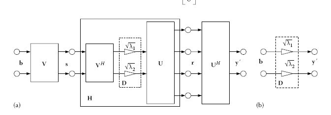
FIGURE 8.10
EBF: The unitary precoding and detection (a) decomposes the equivalent channel into parallel streams (b).

with v₁ the first column of the precoding matrix V. This one-stream beamforming (BF) is also called spot-BF. Even though only one logical MIMO stream carries information, both transmit ports are used since s is a 2 × 1 vector for two transmit ports. One-stream BF might be used if only one receive port is available (MISO) or if the receiver supports only the decoding of one stream (full MIMO with using only one stream). In this case, detection is simplified to a vector multiplication

$W=w=\frac{1}{\sqrt{{\text{λ}}_1}}{u}_1^H$

(8.41)

with u₁ as the first column of U. In the case of a low SINR channel, spot-BF improves the coverage.

Let us go back to the general case b₁ ≠ 0 and b₂ ≠ 0. The precoding matrix V superimposes the symbols of b, and thus the transmit symbol vector s contains all symbols of b, that is, each symbol is transmitted via each MIMO path. Thus, the full spatial diversity N_TN_R is achieved.

U^H is a unitary matrix, that is, the noise variance of n in Equation 8.38 is not affected by the multiplication of U^H if the noise power is the same for all receive ports. D contains the singular values ${\sqrt{\text{λ}}}_p$ on the diagonal, and, from Equation 8.39, it follows that the postdetection SINR of the two streams is

${\mathrm{\Lambda }}_p=\frac{\text{ρ}}{N_T}{\text{λ}}_p,p=1,2.$

(8.42)

If each MIMO stream is modulated independently, the signals of the r_S MIMO streams are uncorrelated

$E\left\{b{b}^H\right\}=I_{r_{\text{S}}}.$

(8.43)

Thus, in the case that no precoding is applied, s = b, the transmitted signals are also uncorrelated $E\left\{s{s}^H\right\}=E\left\{{\left(bb\right)}^H\right\}=I_{N_T}\left(r_{\text{S}}=N_T\right)$. If precoding is applied and the entries of b are uncorrelated, the correlation matrix results in

$E\left\{s{s}^H\right\}=E\left\{\left(Fb\right){\left(Fb\right)}^H\right\}=FE\left\{b{b}^H\right\}{F}^H=F{F}^H.$

(8.44)

In case of EBF with F = V, the unitary property of V simplifies Equation 8.44 to VV^H = I_NT, and the transmit signals are still uncorrelated. If one-stream BF or PA (see next subsection) is used, the simplification is not valid. This results in correlation of the transmit signals. The effect of MIMO transmission on EMI is discussed in Chapters 7 and 16 in detail.

8.5.3    Power Allocation for Spatial Multiplexing Streams

There are basically two options to allocate the total transmit power for MIMO-OFDM systems. The power can be allocated across subcarriers and the power can be distributed among the available MIMO streams. In case of PLC, the first option, the PA across subcarriers, is only possible within the resolution bandwidth used for regulatory assessment (9 kHz for frequencies below 30 MHz and 120 kHz above 30 MHz [32]). EMC regulation accepts a flat power spectral density as maximal feeding level across the subcarriers. Shifting energy between carriers is only possible if subcarrier spacing is smaller than the resolution bandwidth (BW) used for regulatory assessment.

In the following, the second option, the distribution of the total transmit power among the available MIMO streams, is discussed. Water filling (WF) is the optimum MIMO PA to maximise the system capacity [3]. In case that Gaussian distributed input signals are present, the system capacity is maximal. However, if the input signals are taken from a finite set of symbols like QAM, WF is not the optimum solution. Reference [33] derives the optimum PA for arbitrary input distributions and for parallel channels corrupted by additive white Gaussian noise (AWGN). This algorithm is called mercury water filling (MWF). A detailed description of this algorithm goes beyond the scope of this chapter; for details, refer to [33,34]. Only a few key observations are discussed here. The PA coefficients of the MWF algorithm depend on the SNR and modulation scheme of each MIMO stream. The PA coefficients a₁ and a₂ of the two MIMO streams have to meet the constraint:

$a_1+a_2=2.$

(8.45)

Note that the total transmit power P_T is assumed to be constant and that the transmit symbols have average power P_T/2 (see Section 8.3). Equation 8.45 ensures that the total power $\left(a_1+a_2\right)P_T/2=P_T$ is not exceeded.

The PA matrix is constructed by

$P=\left[\begin{array}{cc}\sqrt{a_1}& 0\\ 0& \sqrt{a_2}\end{array}\right].$

(8.46)

Figure 8.11 shows the MWF PA coefficient a₁ (illustrated by the contour lines) depending on the SNR of each MIMO stream and the modulation scheme. Figure 8.11a illustrates binary phase-shift keying (BPSK) and quadrature phase-shift keying (QPSK) modulation on the two MIMO streams while Figure 8.11b shows 16-QAM and 1024-QAM on streams 1 and 2, respectively. According to the WF algorithm, most power is allocated to the MIMO stream with the highest SNR [3]. However, under some circumstances, the MWF algorithm mandates the opposite, as illustrated in Figure 8.11b, for example. Assume that the first stream has an SNR of 15 dB and the second stream an SNR equal to 36 dB. According to Figure 8.11b, more power is assigned to the weaker stream 1 (a₁ = 1.2) than to the stronger stream 2 (a₂ = 0.8).

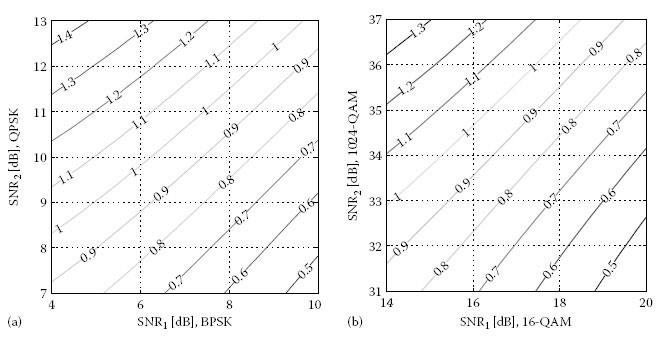
FIGURE 8.11
PA coefficients of mercury water filling (MWF); the contour lines represent the PA coefficient a₁ of the first stream with (a) BPSK and QPSK modulation and (b) 16-QAM and 1024-QAM modulation on the two streams.

A simplified PA algorithm may be used in conjunction with adaptive modulation [18,20]. Only three PA coefficients are used: 0, 1 and $\sqrt{2}$. If one stream of one subcarrier is not allocated any information because of insufficient SNR for the lowest possible constellation, the power is added to the other stream. This results in a 3 dB higher SNR of the boosted stream. If both streams of one subcarrier carry information, the power is equally allocated to the two streams (a₁ = a₂ = 1). The transmitter concludes from the adaptive modulation feedback from the receiver the PA coefficients. Thus, there is no additional feedback of the PA coefficients required. The performance of this simplified PA algorithm is close to optimum MWF (see Section 9.3).

8.5.4    Equivalent Channel and Detection

8.5.4.1    Equivalent Channel Including Precoding

An equivalent channel matrix can be defined, which combines a general precoding matrix F and the channel matrix H as

${\tilde{H}}_{\text{pre}}=HF.$

(8.47)

The detection algorithms introduced in Section 8.5.1 can be applied to the equivalent channel matrix by substituting H by ${\tilde{H}}_{\text{pre}}$.

For the optimum unitary precoding matrix F = V, the different detection algorithms according to Section 8.5.1 yield all the same SINR after detection (see [20]). Thus, if EBF is used, the most simple equaliser (the ZF equaliser) is sufficient. In fact, the ZF equaliser results in W = D⁻¹U^H, which is the same detection matrix as obtained in Section 8.5.2 (see [20]). In case of quantisation of the optimum precoding matrix $F=\tilde{V}$ with $\tilde{V}$ the quantised precoding matrix V, the precoding is no more optimal and more sophisticated equalisers might be used. However, the performance gain of the more sophisticated equalisers compared to ZF detection is very small for a sufficient fine quantisation.

8.5.4.2    Whitening Correlated Noise

Correlation of the noise results in a noise covariance matrix $N_c=E\left\{n{n}^H\right\}$ unequal to the scaled identity matrix. The noise can be whitened by multiplying the received vector r by $N_c^{-\frac{1}{2}}$

$\tilde{r}=N_c^{-\frac{1}{2}}Hs+N_c^{-\frac{1}{2}}n,$

(8.48)

where $N_c^{-\frac{1}{2}}$ is defined such that

$N_c^{-\frac{1}{2}}{N}_c^{-\frac{1}{2}}=N_c^{-1}$

(8.49)

is fulfilled. N_c is a Hermitian matrix, that is, ${\text{N}}_c={\text{N}}_c^H$ since $E{\left\{n{n}^H\right\}}^H=E\left\{n{n}^H\right\}$. A Hermitian matrix N_c can be diagonalised by a unitary matrix U_c [21]:

$N_c=U_c{D}_c{U}_c^H,$

(8.50)

where D_c is a diagonal matrix with real elements. Using $N_c^{-1}=U_c{D}_c^{-1}{U}_c^H,N_c^{-\frac{1}{2}}$ is defined as

$N_c^{-\frac{1}{2}}=U_c{D}_c^{-\frac{1}{2}}{U}_c^H$

(8.51)

with $D_c^{-\frac{1}{2}}$ containing the inverse elements of the square root of the elements of D_c.

Equation 8.51 fulfils Equation 8.49 since $N_c^{-\frac{1}{2}}{N}_c^{-\frac{1}{2}}=U_c{D}_c^{-\frac{1}{2}}{U}_c^H{U}_c{D}_c^{-\frac{1}{2}}{U}_c^H=U_c{D}_c^{-1}{U}_c^H=N_c^{-1}$.

The filtered noise $\tilde{n}=N_c^{-\frac{1}{2}}n$ is uncorrelated with

$E\left\{\tilde{n}{\tilde{n}}^H\right\}=N_c^{-\frac{1}{2}}\underset{N_c}{\underbrace{E\left\{n{n}^H\right\}}}{\left(N_c^{-\frac{1}{2}}\right)}^H\stackrel{\left(0.51\right)}{=}{D}_c^{-1}{D}_c=I_{N_R.}$

(8.52)

The equivalent channel matrix

${\tilde{H}}_{\text{white}}=N_c^{-\frac{1}{2}}H$

(8.53)

can be used to determine the detection matrix and optimum precoding matrix by replacing H by ${\tilde{H}}_{\text{white}}$.

8.6    Simulation Results

The MIMO-OFDM system described in Section 8.3 forms the basis of the system simulations. 1296 subcarriers are used in the frequency range from 4 to 30 MHz^*.

The noise is modelled by AWGN with zero mean, and it is assumed that the noise is uncorrelated and that the noise power is the same for all receive ports. The transmit power to noise power level is assumed to be ρ = 65 dB. This value corresponds to transmit power spectral density of −55 dBm/Hz (see Chapter 6) and an average noise power spectral density of −120 dBm/Hz (this corresponds to the 90% point of CDF of the noise according to Chapter 5). Impulsive noise is not considered. The focus is on the comparison between MIMO and SISO schemes. It is expected that impulsive noise will influence all receive ports in a similar way. Thus, mitigation techniques known from SISO systems can be applied [23,35]. The measured MIMO PLC channels obtained during the European measurement campaign (ETSI STF410, see Chapter 5) are used in the system simulations. In case of MIMO, the two feeding ports D₁ and D₃ (i.e. L-N and L-PE; see Chapter 5) and all four receive ports (S₁ S₂, S₃, S₄) are used; in case of SISO, the D₁ (L-N) port is used at the transmitter and the S₁ port (L) at the receiver. It was observed that using the S₂ port (N) at the receiver yields the same performance as using the S₁ port. The corresponding SNR is calculated based on the channel matrix of each subcarrier (channel estimation is assumed to be perfect), depending on the MIMO scheme as shown in the previous sections.

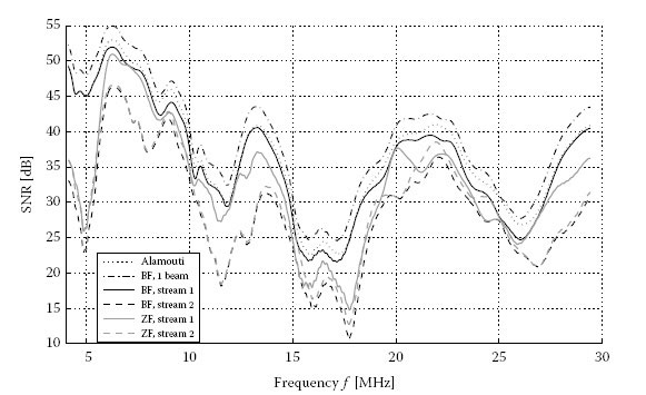
FIGURE 8.12
Frequency-dependent SNR for multiplexing streams 1 and 2 of different MIMO schemes, ρ = 65 dB, N_T = 2, N_R = 4.

Figure 8.12 compares the SNR after detection for different MIMO schemes: the Alamouti scheme, SMX with ZF detection and BF with one and two streams. The precoding matrix in case of BF is assumed to be perfect. A typical MIMO channel is shown in the figure. No PA is applied for the schemes with two streams.

The SNR after detection is still very frequency selective for all the MIMO schemes shown. BF with one stream (spot-BF) and the Alamouti scheme achieve the highest SNR. However, these two schemes support only one MIMO stream. This has to be kept in mind with respect to the achieved bitrate (see Section 9.3). The SMX schemes provide two MIMO streams. For SMX without precoding (ZF in the figure), there is no preferred spatial stream; the two streams range in the same order of SNR. Consider the frequencies between 20 and 25 MHz: For some frequencies, the first stream offers higher SNR than the second one and vice versa. Precoding (BF) enforces one of the streams and weakens the other stream. However, the gain of stream 1 is much higher compared to the loss of the second stream. This behaviour is especially visible for the low frequencies of this channel. This results in higher bitrates for precoding (see Chapter 9). The SNR curve of one-stream BF is shifted by 3 dB compared to the first stream of EBF. The second stream is not used, and therefore the power is assigned completely to the first stream.

Figure 8.13 presents the SNR after detection of different SMX schemes. The two MIMO streams are shown in Figure 8.13a and b for the first and second streams, respectively. To show the advantage of MMSE, the same channel is used as in Figure 8.12 with a lower transmit to noise power level of ρ = 44 dB to make the effects of very low SNR more visible. The gain of BF is again visible for the first stream, as already discussed earlier. ZF detection and SIC yield the same SNR for the first stream since the detection of the first stream is performed in the same way (see Section 8.5.1). The gain of SIC becomes visible for the second stream. MMSE detection improves the SNR only in very poor SNR regions (see frequencies around 17 MHz). For high SNR regions, the MMSE gain diminishes compared to ZF. The gain of OSIC (not shown in the figures) is only marginal compared to SIC.

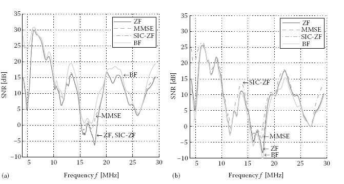
FIGURE 8.13
Frequency-dependent SNR of stream 1 (a) and stream 2 (b) of different spatial multiplexing MIMO schemes, same channel as in Figure 8.12, ρ = 44 dB, N_T = 2, N_R = 4.

Figure 8.14 compares the SNR of PA for BF and SIC. The top row of the figure illustrates the SNR; the lower row shows the PA coefficients of MWF. For frequencies with very low SNR on the second stream, no information is assigned by the adaptive modulation to the second stream. The complete power is assigned to the first stream. The PA coefficient of the first stream becomes 2 while the PA coefficient of the second stream becomes 0 (see Figure 8.14c). For these frequencies, two-stream BF falls back to one-stream BF (see Figure 8.14a). The SNR of the two streams of SIC is closer together compared to BF (see Figure 8.14b). Thus, the variation of the PA coefficients is not that pronounced and the extreme PA coefficients 0 and 2 do not appear that often compared to BF. The gain of PA for EBF is higher, compared to SMX without precoding. The same behaviour is observed for the other SMX schemes (ZF and MMSE, data not shown). The gain of PA becomes smaller for higher SNR.

Figure 8.15 shows the cumulative distribution function (CDF) of the SNR of all MIMO PLC channel measurements. No PA is applied. The spatial streams are drawn separately. One spatial stream is available for SISO and the Alamouti scheme, while the SMX schemes with ZF, SIC-ZF and EBF have two spatial streams. The Alamouti scheme and the first spatial stream of EBF give the highest SNR. Note that Alamouti uses only one spatial stream, while EBF offers a second spatial stream which can be used for communication. The second spatial stream has the lowest SNR in Figure 8.15. EBF maximises the first spatial stream. Although the second stream is weakened, the sum of both streams offers the highest performance, which is shown for the throughput results in Chapter 9 the SNR gain of EBF is most visible for the low SNR region which is most important to increase the coverage. The SNR values of the two streams of SMX with ZF detection (SMX-ZF) are in the same order of magnitude. This is due to the fact that SMX has no preference with respect to the spatial streams. At the median point, the SNR is about 3 dB lower compared to SISO. The SNR of the first spatial stream of SIC-ZF is exactly the same as ZF since the first stream is detected in the same way. However, the SNR of the second spatial stream is increased by 7 dB in median compared to the second stream of ZF.

FIGURE 8.14
SNR for spatial multiplexing streams 1 and 2 for BF (a) and SIC (b), and corresponding power allocation (PA) coefficients for BF (c) and SIC (d) as a function of frequency, same channel as in Figure 8.12, ρ = 44 dB, N_T= 2, N_R = 4.

Figure 8.16 shows the CDF for the SMX schemes with different detection algorithms and EBF. Additionally to ZF, SIC-ZF and EBF as already illustrated in Figure 8.15, MMSE and SIC-MMSE are shown. As for ZF and SIC-ZF, the SNR of the first spatial stream of MMSE and SIC-MMSE are identical. MMSE offers only an increased SNR for low SNR regions (gain of 4 dB at the 10% point), while for moderate toward high SNR, ZF and MMSE converge to the same performance. Comparing the best detection scheme which is SIC-MMSE to EBF leads to the following conclusions. At the high SNR region, the gain of the first stream of EBF compared to the stronger stream of SIC-MMSE is similar to the loss of EBF’s second stream compared to the weaker stream of SIC-MMSE. This indicates that the same throughput could be expected for these two schemes for low attenuated channels (see also the Section 9.3) when neglecting any error propagation in SIC-MMSE due to wrongly decided symbols in the first iteration of the SIC algorithm. However, at the low SNR region, due to the fact that EBF maximises the first stream, the first EBF stream might carry information while the SNR of the two streams of SIC- MMSE might be too low for communication (again refer to Section 9.3).

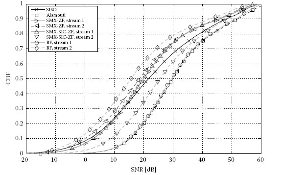
FIGURE 8.15
Cumulative distribution function (CDF) of the SNR for multiplexing streams 1 and 2 of different MIMO schemes and SISO, ρ = 65 dB, N_T = 2, N_R = 4.

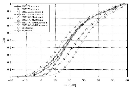
FIGURE 8.16
Cumulative distribution function (CDF) of the SNR for multiplexing streams 1 and 2 of different two-stream MIMO schemes, ρ = 65 dB, N_T = 2, N_R = 4.

TABLE 8.1

Qualitative Comparison of Different MIMO Schemes for PLC

a  SISO with SD requires several transmit ports or several receive ports; however, only one stream is processed.

Table 8.1 shows a qualitative comparison and summary of the different MIMO schemes and illustrates the pros and cons with respect to MIMO PLC. The MIMO schemes discussed in this chapter are shown in the first column. The second column shows the minimum required configuration of transmit and receive ports. SISO is considered as a special MIMO configuration with one transmit and one receive port. SISO with selection diversity (SD) uses several transmit or receive ports at the coupler. However, only one of the transmit or receive streams is processed which makes the signal processing a SISO scheme. The Alamouti scheme requires two transmit ports and at least one receive port, that is, a MISO configuration is sufficient. The SMX schemes use two spatial modes, that is, at least two transmit and two receive ports are needed, the same holds for EBF. Spot BF utilises only one spatial stream. Thus, a MISO configuration is sufficient, at least two transmit ports are required to form the beam. The third and fourth columns show the achievable performance in the high coverage area (for channels with low SNR) and in the low coverage area where the maximum throughput could be achieved (for channels with high SNR), respectively. Compared to the SISO reference, the Alamouti scheme achieves very good performance for low SNR channels; however, no multiplexing gain is achieved for channels with high SNR due to the transmission of only one spatial stream. The SMX schemes use two spatial streams and therefore good performance is achieved for high SNR channels. The performance for low SNR channels depends on the MIMO detection algorithm or equaliser. The most simple detection algorithm is ZF which results in poor SNR after detection for highly correlated channels. The more sophisticated detection algorithms MMSE, SIC-ZF, SIC-MMSE, OSIC-ZF and OSIC-MMSE increase the performance if real- world imperfections are not considered. The BF schemes achieve the highest performance for all channel conditions since the transmission is optimally adopted to the channel by the precoding. The first spatial stream is maximised, which gives the best performance for low SNR channels. For high attenuated channel, the second spatial stream has only low SNR after detection. Thus, one-stream and two-stream BF achieve almost the same performance in the high coverage area. For low attenuated channels, one-stream BF does not achieve the multiplexing gain and two-stream BF outperforms one-stream BF. The last three columns compare the MIMO schemes in terms of complexity. The BF schemes usually require feedback from the receiver to the transmitter. This feedback is no significant drawback for PLC as will be discussed in the conclusions. With respect to the implementation complexity at the transmitter and receiver, the SISO complexity serves as reference with very low complexity. The Alamouti scheme and SMX schemes without precoding require a de-multiplexing to split the incoming bits or QAM symbols to the two transmit ports. BF applies precoding at the transmitter which is a matrix multiplication. At the receiver, the Alamouti decoding is basically a matrix multiplication making use of the orthogonal property of the Alamouti code. The detection complexity of the SMX schemes increases with the more sophisticated equaliser algorithms. For BF, the most simple detection algorithm is sufficient which is ZF detection. For one-stream BF, the complexity is further reduced since only one spatial stream has to be decoded.

8.7    Conclusions

This chapter introduced MIMO signal processing theory and its application to MIMO PLC. The comparison of several MIMO schemes aimed at answering the question which MIMO scheme is suited best for in-home PLC. Although the investigations focused on in-home PLC, many aspects and conclusions may also apply to access PLC. The SNR after MIMO processing at the receiver was investigated. The Alamouti scheme improves the SNR compared to SISO. However, no multiplexing gain is achieved because of the transmission of replicas of each symbol. SMX uses two spatial streams and different detection algorithms were investigated. ZF detection is the most simple detection scheme. However, ZF detection fails for a high correlation of the channel which results in low SNR after detection, which might be even below the SNR of SISO for high spatial correlation. More complex detection algorithms (like MMSE and SIC) improve the performance of the SMX schemes. In particular, the SIC receiver approaches the BF performance for channels with low attenuation. However, the general problem for correlated channels remains.

BF offers the highest SNR under all channel conditions by adapting the transmission to the eigenmodes of the channel. The full spatial diversity gain is achieved for highly attenuated channels while the SMX gain is achieved for channels with low attenuation. The most simple detection algorithm, which is ZF detection, can be used in case of BF since the performance of BF is independent of the detection algorithm. Spatial correlation of the transmit signals may cause higher radiation emission of the power lines. However, the unitary precoding matrix of EBF does not introduce any correlation of the transmit signals if the two streams before precoding are uncorrelated. Chapter 16 investigates the influence of spot BF on the EMI. BF offers flexibility with respect to the receiver configuration. Only one spatial stream may be activated by the transmitter if only one receive port is available, that is, if the outlet is not equipped with the third wire or if a simplified receiver implementation is used which supports only one spatial stream. Since BF aims to maximise one MIMO stream, the performance loss of not utilising the second stream is relatively small compared to the SMX schemes without precoding. This is especially true for highly attenuated and correlated channels, where the SNR of the second MIMO stream is very low and no information might be carried on this stream. These channels are most critical for PLC coverage and adequate MIMO schemes are important. BF uses CSI at the transmitter. Usually, the CSI in terms of the precoding matrix is fed back from the receiver to the transmitter. Due to this feedback, BF is also called a closed-loop MIMO scheme in contrast to the open-loop MIMO schemes which do not use CSI at the transmitter. The feedback creates an additional overhead. However, the feedback of the precoding matrix can be combined with the feedback of the tone maps for adaptive modulation (see Chapter 9). Additionally, the update rate of the feedback is low since the time variations of the PLC channel are low (for changes in the network topology) or periodic within a line cycle. The amount of feedback to quantise the precoding matrix without performance loss is investigated in [18,20].

The throughput results of the different MIMO schemes are investigated in Chapter 9. In particular, the SNR after detection is used to apply adaptive modulation and to calculate the achieved bitrate. HomePlug and ITU-T G.hn adopted MIMO and precoded SMX or BF in their next-generation specifications HomePlug AV2 (see Chapter 14) and G.hn/G.9963 (see Chapter 12), respectively.

References

1.  G. J. Foschini, Layered space–time architecture for wireless communication in a fading environment when using multi-element antennas, Bell Labs Tech. J., 1(2), 41–59, 1996.

2.  I. E. Telatar, Capacity of multi-antenna Gaussian channels, Eur. Trans. Telecom., 10, 585–595, 1999.

3.  A. Paulraj, R. Nabar and D. Gore, Introduction to Space–Time Wireless Communications. Cambridge University Press, Cambridge, U. K., 2003.

4.  L. Schumacher, L. T. Berger and J. Ramiro Moreno, Recent advances in propagation characterisation and multiple antenna processing in the 3 GPP framework, in XXVIth URSI General Assembly, Maastricht, the Netherlands, August 2002, session C2. [Online] Available: http://www.ursi.org/Proceedings/ProcGA02/papers/p0563.pdf.

5.  C. L. Giovaneli, P. F. J. Yazdani and B. Honary, Application of space–time diversity/coding for power line channels, in International Symposium on Power Line Communications and Its Applications, Athens, Greece, 2002, pp. 101–105.

6.  C. L. Giovaneli, P. G. Farrell and B. Honary, Improved space–time coding applications for power line channels, in International Symposium on Power Line Communications and Its Applications, Kyoto, Japan, 2003, pp. 50–55.

7.  C. L. Giovaneli, B. Honary and P. G. Farrell, Optimum space-diversity receiver for Class A noise channels, in International Symposium on Power Line Communications and Its Applications, Zaragoza, Spain, 2004, pp. 189–194.

8.  A. Papaioannou, G. D. Papadopoulos and F.-N. Pavlidou, Performance of space–time block coding over the power line channel in comparison with the wireless channel, in International Symposium on Power Line Communications and Its Applications, Zaragoza, Spain, 2004, pp.362–366.

9.  A. Papaioannou, G. D. Papadopoulos and F. -N. Pavlidou, Performance of space-time block coding in powerline and satellite communications, J. Commun. Inf. Syst., 20(3), 174–181, 2005.

10.  C. Giovaneli, B. Honary and P. Farrell, Space–frequency coded OFDM system for multi-wire power line communications, in International Symposium on Power Line Communications and Its Applications, Vancouver, British Columbia, Canada, April 2005, pp. 191–195.

11.   B. Adebisi, S. Ali and B. Honary, Multi-emitting/multi-receiving points MMFSK for power-line communications, in International Symposium on Power Line Communications and Its Applications, Dresden, Germany, 2009, pp. 239–243.

12.  L. Hao and J. Guo, A MIMO-OFDM scheme over coupled multi-conductor power-line communication channel, in International Symposium on Power Line Communications and Its Applications, Pisa, Italy, 2007, pp. 198–203.

13.  H. Furukawa, H. Okada, T. Yamazato and M. Katayama, Signaling methods for broadcast transmission in power-line communication systems, in International Symposium on Power Line Communications and Its Applications, Kyoto, Japan, 2003.

14.  F. de Campos, R. Machado, M. Ribeiro and M. de Campos, MISO single-carrier system with feedback channel information for narrowband PLC applications, in International Symposium on Power Line Communications and Its Applications, Dresden, Germany, 2009, pp. 301–306.

15.  M. Kuhn, D. Benyoucef and A. Wittneben, Linear block codes for frequency selective PLC channels with colored noise and multiple narrowband interference, in Vehicular Technology Conference, VTC Spring 2002, vol. 4, Birmingham, AL, 2002, pp. 1756–1760.

16.  L. Lampe, R. Schober and S. Yiu, Distributed space–time coding for multihop transmission in power line communication networks, IEEE J. Sel. Areas Commun., 24(7), 1389–1400, 2006.

17.  L. Stadelmeier, D. Schneider, D. Schill, A. Schwager and J. Speidel, MIMO for inhome power line communications, in International Conference on Source and Channel Coding (SCC), ITG Fachberichte, Ulm, Germany, 2008.

18.  D. Schneider, J. Speidel, L. Stadelmeier and D. Schill, Precoded spatial multiplexing MIMO for inhome power line communications, in Global Telecommunications Conference, IEEE GLOBECOM, New Orleans, LA, 2008.

19.  A. Canova, N. Benvenuto and P. Bisaglia, Receivers for MIMO-PLC channels: Throughput comparison, in International Symposium on Power Line Communications and Its Applications, Rio de Janeiro, Brazil, 2010, pp. 114–119.

20.  D. Schneider, Inhome power line communications using multiple input multiple output principles, Dr.-Ing. dissertation, Verlag Dr. Hut, January 2012.

21.  R. A. Horn and C. R. Johnson, Matrix Analysis. Cambridge University Press, Cambridge, U.K., 1985.

22.  J. Proakis, Digital Communications, 4th edn. McGraw-Hill Book Company, New York, 2001.

23.  E. Biglieri, Coding and modulation for a horrible channel, IEEE Commun. Mag., 41(5), 92–98, 2003.

24.  S. Alamouti, A simple transmit diversity technique for wireless communications, IEEE J. Sel. Areas Commun., 16(8), 1451–1458, 1998.

25.  B. Vucetic and J. Yuan, Space–Time Coding. John Wiley, Chichester, U.K., 2003.

26.  W. Zhang, X.-G. Xia, P. Ching and H. Wang, Rate two full-diversity space–frequency code design for MIMO-OFDM, in Workshop on Signal Processing Advances in Wireless Communications, New York, June 2005, pp. 303–307.

27.  W. Zhang, X.-G. Xia and P. C. Ching, High-rate full-diversity space–time–frequency codes for broadband MIMO block-fading channels, IEEE Trans. Commun., 55(1), 25–34, January 2007.

28.  E. Viterbo and J. Boutros, A universal lattice code decoder for fading channels, IEEE Trans. Inf. Theory, 45(5), 1639–1642, July 1999.

29.  A. Paulraj, D. Gore, R. Nabar and H. Bolcskei, An overview of MIMO communications – A key to gigabit wireless, Proc. IEEE, 92(2), 198–218, February 2004.

30.  A. Boronka, Verfahren mit adaptiver Symbolauslschung zur iterativen Detektion codierter MIMO-Signale, Dr.-Ing. dissertation, Institute of Telecommunications, University of Stuttgart, November 2004.

31.  A. Scaglione, P. Stoica, S. Barbarossa, G. Giannakis and H. Sampath, Optimal designs for space–time linear precoders and decoders, IEEE Trans. Signal Process., 50(5), 1051–1064, May 2002.

32.  CISPR 16-1:1999: Specification for radio disturbance and immunity measuring apparatus and methods. Radio disturbance and immunity measuring apparatus, CISPR Std.

33.   A. Lozano, A. Tulino and S. Verdu, Mercury/waterfilling: Optimum power allocation with arbitrary input constellations, in International Symposium on Information Theory, Adelaide, South Australia, Australia, 2005, pp. 1773–1777.

34.  A. Lozano, A. Tulino and S. Verdu, Optimum power allocation for parallel Gaussian channels with arbitrary input distributions, IEEE Trans. Inf. Theory, 52(7), 3033–3051, 2006.

35.  D. Fertonani and G. Colavolpe, On reliable communications over channels impaired by bursty impulse noise, IEEE Trans. Commun., 57(7), 2024–2030, 2009.

*  The singular values ${\sqrt{\text{λ}}}_p,$ are derived from the eigenvalues λ_p of H^HH.

*  This is only true if the channel matrix has full rank; otherwise, the number of spatial streams is limited by the rank R′ of the channel matrix r_S ≤ R′.

*  The optimum precoder is derived in [31] by minimising the MSE matrix:

*  The system uses a 2048 OFDM from 0 to 40 MHz with 1296 active subcarriers in the frequency range from 4 to 30 MHz. The other subcarriers are not active.

*  Alternative implementations use an inverse fast Fourier transform (IFFT) of double size with complex conjugate input to obtain the real-valued signal which is often referred to as discrete multi-tone modulation (DMT). In this case, frequency up-conversion is not needed.

with y, b, F, W and H from Equation 8.35 and the covariance matrices $R_{bb}=E\left\{b{b}^H\right\}$ and $R_{nn}=E\left\{n{n}^H\right\}$.