20. Relaying Protocols for In-Home PLC

Power saving is playing an important role in the development of advanced communication devices. For instance, the IEEE 802.3az Ethernet standard [1] and the HomePlug Green physical (PHY) (GP) power line communication (PLC) specifications (HomePlug GP [2]) have been developed to specifically address this problem. Not only power saving but also high transmission rate has to be granted, for instance, in multimedia applications such as high-definition television (HDTV) or 3D virtual video games. It therefore becomes essential to consider advanced communication techniques such as multi-carrier modulation with bit and power loading algorithms, cooperative communication algorithms and cross-layer optimisation.

In this chapter, we investigate the use of cooperative half-duplex time division relay protocols to possibly provide power savings, achievable rate improvements and coverage extension to the in-home PLC networks whose communication devices adopt multicarrier modulation at the PHY layer, that is, orthogonal frequency division multiplexing (OFDM) [3].

20.1.1 Related Literature

In relay networks, the communication between the source and the destination nodes is helped by the use of one or more relays. More precisely, the relay receives the signal addressed to the destination node, processes it according to a given relay protocol and forwards it to the destination. The destination node combines the signals received from the source and from the relay. Many relay protocols have been proposed in the literature [4]: amplify and forward (AF), classic multi-hop, compress and forward (CF), decode and forward (DF) and multipath DF. In the following, we focus on AF and DF. In AF, the relay only amplifies and forwards the received signal to the destination, whereas in DF, the relays decode and re-encode the signal before forwarding it. AF and DF have been studied considering both half-duplex and full-duplex transmission, namely, a node can only transmit or receive at one time, or it can transmit and receive simultaneously. In the rest of this chapter, we consider the half-duplex modality, since full duplex is often not possible to be implemented due to high complexity [4].

The problem of resource allocation in relay networks has been thoroughly treated in the wireless literature. In the following, a number of relevant papers on the topic are reported.

The optimal power and time slot allocation for capacity maximisation over Rayleigh fading relay channels has been considered in Refs. [5,6,7]. The case of power allocation for capacity maximisation of single-hop parallel Gaussian relay channels (e.g. OFDM systems) under a total power constraint has been treated in Refs. [8,9,10,11,12]. In particular, in Ref. [8], the authors found a suboptimal power allocation considering half-duplex AF and a total power constraint at the source and relay nodes. The optimal solution to the previous problem has been found in Ref. [9]. In Ref. [11], the authors found the optimal power allocation for half-duplex AF and DF under a total power constraint (source plus relay) in each OFDM sub-channel. Both previous papers assume that the destination node is not directly reachable from the source. In Ref. [12], the power allocation for full-duplex DF [5] under a total power constraint (source and relay) is considered. The optimal power allocation for the hybrid use of AF, DF and direct link transmission is computed in Ref. [10] under a source plus relay power constraint in each sub-channel. In Ref. [13], the authors found the optimal power allocation for full- and half-duplex DF under a total power constraint at the source and destination nodes. Cooperation with multiple relays or relays with multiple antennas has been extensively treated in the wireless literature (cf., e.g. [14,15] and references therein).

In this chapter, we consider the specific and peculiar application of relaying in the in-home PLC scenario. In contrast to the wireless case, the use of cooperative communication schemes for PLC has not been deeply investigated yet. In the following, we report a list of relevant papers.

The use of repeaters over large-scale PLC networks, namely, networks where the source and destination nodes are far apart so that they cannot directly communicate, was proposed in Ref. [16] and extended in Ref. [17]. In particular, the use of the single-frequency network flooding approach was advocated to simplify the transmission of data by multiple relays. In Ref. [18], the authors considered the application of distributed space–time coding to the single-frequency network consisting of multiple relays to improve the network performances in terms of required transmit power and multi-hop delay. Different geographic routing schemes – namely, routing schemes that make use of the location of PLC devices – for low-data-rate Smart Grid applications over low- and medium-voltage distribution grids, were compared in Ref. [19] and optimised in Ref. [20]. In Ref. [21], the authors studied the diversity gains – namely, the asymptotic decay of the outage rate as a function of the signal to noise ratio (SNR) – over single-hop PLC relay networks. In particular, they found that no diversity gains are, in general, attainable in the examined context. This result is due to the peculiar electrical characteristics of the PLC network which behaves similarly to the keyhole channel observed in some MIMO wireless contexts. Despite the previous result, as it will be also shown in the following, in general, the use of relays in PLC networks leads to significant capacity gains w. r.t. the direct transmission (DT). Resource allocation algorithms were presented in Ref. [22], where the authors proposed practical sub-channel and power allocation algorithms for a two-hop DF relay scheme to improve the achievable rate of an orthogonal frequency division multiple access (OFDMA) PLC in-home network. The numerical results were obtained using a small number of measured channels and assuming a total power constraint at each network node. Achievable rate comparisons for AF and DF schemes over PLC channels were reported in Ref. [23], where it was assumed that the network nodes employed OFDM at the PHY layer and the power was equally distributed among the used OFDM sub-channels. Numerical results showed that the use of half-duplex single-relay schemes leads to marginal improvements of the achievable rate w. r.t. the DT. However, this result is only partially true, since the opportunistic use of the relay was not considered and the dependency on the relay position was not thoroughly investigated. Finally, in Ref. [24], the authors extended the work by considering the effect of channel estimation errors.

20.1.2 Chapter Contribution

In this chapter, we consider a network whose nodes have a PHY layer based on OFDM and where the communication between the source and the destination nodes follows an opportunistic protocol, namely, the relay is used whenever it allows (w.r.t. the DT): (1) for achievable rate improvements under a power spectral density (PSD) mask constraint or (2) for power saving under a PSD mask and a rate target constraint. Opportunistic decode and forward (ODF) and opportunistic amplify and forward (OAF) are considered. As it is typically required by state-of-the-art communication standards, for example, the wireless IEEE 802.11 standard, the power line IEEE 1901 standard and the twisted pair xDSL standard, we assume that the signal transmitted by the network nodes has to satisfy a PSD mask [25]. Under these assumptions and a Gaussian noise model, we find the optimal resource allocation, namely, the optimal power and time slot allocation, at the source and relay nodes that maximises the achievable rate or minimises the total transmitted power for both ODF and OAF.

Furthermore, for the specific and peculiar in-home PLC scenario, we consider the optimal relay positioning. In fact, differently from the wireless case, where the relay can be placed wherever between the source and the destination nodes, in in-home PLC networks, the relay can only be placed in accessible points of the network, that is, in the outlets or in the main panel (MP) or, in principle, in accessible derivation boxes (boxes where wires are connected to generate branches or extensions).

The remainder of the chapter is as follows. In Section 20.2, we describe the adopted PLC system model. Then, in Sections 20.3 and 20.4, we, respectively, consider the resource allocation problem of ODF and OAF. Section 20.5 discusses numerical results. Finally, a summary of the findings follows in Section 20.6.

20.2 PLC System Model

We consider an in-home PLC network where the communication between the source (S) and the destination (D) nodes exploits the use of a relay (R) (see Figure 20.1; the meaning of the variables in Figure 20.1 is explained in the following). In particular, we consider that the communication between the source and the destination nodes follows an opportunistic cooperative protocol, namely, the relay is used whenever it allows, according to the goal, for rate improvements or for power saving w. r.t. the DT. The multiplexing between the source and the relay nodes is accomplished via time division multiple access (TDMA). The time is divided in frames of duration T_f, and each frame is divided into two time slots whose durations are τ and T_f − τ. When the relay is used, the source transmits its data to the relay and destination nodes during the first slot – although it is possible that the source cannot directly reach the destination – whereas, during the second slot, the source is silent and the relay transmits the received data to the destination according to the adopted opportunistic cooperative protocol, that is, ODF or OAF. When ODF is used, the relay decodes, re-encodes and forwards the received data using an independent codebook [6,26], whereas, in OAF, the relay only amplifies and forwards the data (see Figure 20.2).

At the PHY layer, we assume OFDM with M sub-channels. The channel frequency response between each pair of nodes is denoted as $H_{x, y}^{(k)}$ $H_{x, y}^{(k)}$ , where the subscripts x and y denote the pairs {S,R}, {S,D} or {R,D} and k is the sub-channel index, that is, k ∈ K_on, where K_on is the subset of used (switched on) sub-channels that allows for satisfying a PSD mask with notches, as it is the case in broadband and narrowband PLC systems [27,28]. Therefore, the received signal in the kth sub-channel of the yth node reads

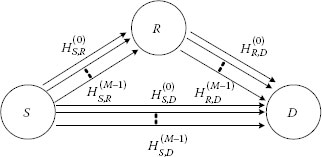
FIGURE 20.1
Two-hop relay network.

FIGURE 20.2
Time slot allocation for DT, DF and AF.

$\begin{matrix} z_{y}^{(k)} = a_{x}^{(k)} H_{x, y}^{(k)} + w_{y}^{(k)}, & {x, y} \in {{S, D}; {S, R}; {R, D}}, & k \in K_{o n} \end{matrix},$ $\begin{matrix} z_{y}^{(k)} = a_{x}^{(k)} H_{x, y}^{(k)} + w_{y}^{(k)}, & {x, y} \in {{S, D}; {S, R}; {R, D}}, & k \in K_{o n} \end{matrix},$

(20.1)

where

$a_{x}^{(k)}$ $a_{x}^{(k)}$ is the symbol transmitted by node x in sub-channel k using DT, DF or AF modes

$w_{x}^{(k)}$ $w_{x}^{(k)}$ is the background noise

We assume the noise and the transmitted symbols to be independent and identically distributed (i. i. d.) and drawn from normal Gaussian distributions with zero mean and power $P_{w, y}^{(k)}$ $P_{w, y}^{(k)}$ and $P_{x, m o d e}^{(k)}$ $P_{x, m o d e}^{(k)}$ respectively.* In the remainder of this section, we assume the application of a PSD mask constraint for the signal transmitted by the network nodes. Furthermore, in order to simplify the notation, we assume the PSD to be constant over the sub-channels, that is, $P_{x, m o d e}^{(k)} \leq \overset{⇀}{P} \forall k \in K_{o n}, x \in {S; R}$ $P_{x, m o d e}^{(k)} \leq \overset{⇀}{P} \forall k \in K_{o n}, x \in {S; R}$ and mode ∈ {DT;DF;AF}. We highlight that all the power allocation algorithms that will be presented are also valid when a more general nonconstant PSD is considered.

20.2.1 In-Home Power Line Network Topology

As discussed in Section 20.1, we are interested to see whether achievable rate improvements, power savings and coverage extension are attainable through the use of ODF and OAF. To this end, in the following, we describe a typical PLC network topology, which allows for understanding where relays can be placed, and it highlights the differences with the wireless context. It is representative of the majority of Italian and EU residential wiring structures [29]. In particular, it is characterised by a wiring topology composed of two layers. As shown in Figure 20.3, the outlets are placed at the bottom layer and are grouped and fed by the same ‘super node’, which is referred to as derivation box. All the outlets fed by the same derivation box are nearby placed. Therefore, the location plan is divided into elements denoted as ‘clusters’ that contain a derivation box with the associated outlets. Each cluster represents a room or a small number of nearby rooms. Different clusters are usually interconnected through their derivation boxes with dedicated cables. This set of interconnections forms the second layer of the topology. We refer to the channels that connect a pair of outlets belonging to the same cluster as intracluster channels, whereas the channels associated to pairs of outlets that belong to different clusters are referred to as intercluster channels. An intercluster channel example is shown in Figure 20.3.

The MP plays a special role inasmuch as it connects the home network with the energy supplier network (not shown in Figure 20.3) through circuit breakers (CBs). We distinguish two cases. The first case, which we refer to as single-sub-topology networks, is when a single CB feeds all the derivation boxes of the home network. The second case, which we refer to as multi-sub-topology networks, is when many sub-topologies, each comprising a group of derivation boxes, have their own electrical circuit that is interconnected at the MP through a CB. The latter case can be, for instance, representative of a multi-floor house, where each floor is a sub-topology. In Figure 20.3, we report an example of a two-sub-topology network.

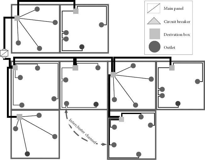
FIGURE 20.3
In-home network with two sub-topologies where each sub-topology is fed by a CB.

Now, we consider the communication between source and destination nodes with the help of a relay. In particular, we consider source–destination channels defined between pairs of outlets that do not belong to the same cluster, that is, intercluster channels. As shown in Ref. [30] these channels experience higher attenuations than intracluster channels. Thus, they can benefit more from the presence of a relay. Clearly, these benefits are also dependent on the relay location. To this end, for single-sub-topology networks, the relay can be strategically placed in the following manners:

• Outlet relay arrangement (ORA). The relay is placed in a randomly selected network outlet.

• Main panel single sub-topology (MPS). The relay is placed immediately after the CB of the MP.

• Random derivation box (RDB). The relay is placed in a randomly selected network derivation box. In general, derivation boxes are accessible although they do not have an already installed outlet. Thus, a relay can be installed inside the box or nearby.

• Backbone derivation box (BDB). The relay is located in a randomly selected derivation box that belongs to the backbone between the source and the destination nodes. Note that, for intercluster channels, the source and destination nodes are at least divided by the source and destination derivation boxes (DDBs).

• Source derivation box (SDB). The relay is located in the derivation box that feeds the source node. Note that for intercluster channels, the path between source and destination includes at least the derivation box that feeds the source and the one that feeds the destination.

• DDB. The relay is located in the derivation box that feeds the destination node.

When we consider multi-sub-topology networks, we assume that the source and the destination node are located in two different sub-topologies. In such a case, we can consider the following strategical configurations for the relay:

• Main panel multi-sub-topology (MPM). The relay is located between the CBs that feed the sub-topologies.

• Outlet relay arrangement source sub-topology (ORAS). The relay is located in a randomly selected outlet belonging to the same sub-topology of the source node.

• Outlet relay arrangement destination sub-topology (ORAD). The relay is located in a randomly selected outlet belonging to the same sub-topology of the destination node.

20.3 Opportunistic Decode and Forward

In ODF, the source node sends data to the destination node according to two modes: DT or DF. Assuming a frame of normalised duration T_f = 1, we can compute the achievable rate of ODF as [6]

$C_{O D F} (τ) = \max {C_{D T}, C_{D F} (τ)},$ $C_{O D F} (τ) = \max {C_{D T}, C_{D F} (τ)},$

(20.2)

where C_DT and C_DF(τ), respectively, denote the capacity of DT and the achievable rate of DF [5]. These are given by

$C_{D T} = C_{S, D},$ $C_{D T} = C_{S, D},$

(20.3)

$C_{D F} (τ) = \min {\underset{f_{1} (τ, P_{S,DF})}{\underset{︸}{τ C_{S, R}}}, \underset{f_{2} (τ, P_{S,DF}, P_{R,DF})}{\underset{︸}{τ C_{S, D} + (1 - τ) C_{R, D}}}} .$ $C_{D F} (τ) = \min {\underset{f_{1} (τ, P_{S,DF})}{\underset{︸}{τ C_{S, R}}}, \underset{f_{2} (τ, P_{S,DF}, P_{R,DF})}{\underset{︸}{τ C_{S, D} + (1 - τ) C_{R, D}}}} .$

(20.4)

In Equations 20.3 and 20.4, C_S,D, C_S,R and C_R,D denote the capacities of the links S–D, S–R and R–D, respectively; furthermore, the minimisation in Equation 20.4 is due to the fact that in DF mode, we require both the relay and the destination to decode the signal, and the unitary term is given by T_f = 1. Now, assuming the system model of Section 20.2, they are given by Ref. [26]

$C_{x, y} = \frac{1}{M T} \sum_{k \in K_{o n}} \log_{2} (1 + {SNR}_{x, y}^{(k)}), {x, y} \in {{S, D}; {S, R}; {R, D}},$ $C_{x, y} = \frac{1}{M T} \sum_{k \in K_{o n}} \log_{2} (1 + {SNR}_{x, y}^{(k)}), {x, y} \in {{S, D}; {S, R}; {R, D}},$

(20.5)

where

$S N R_{x, y}^{(k)} = P_{x, m o d e}^{(k)} \frac{| H_{x, y}^{(k)} |}{P_{w, y}^{(k)}} = P_{x, m o d e}^{(k)} η_{x, y}^{(k)}$ $S N R_{x, y}^{(k)} = P_{x, m o d e}^{(k)} \frac{| H_{x, y}^{(k)} |}{P_{w, y}^{(k)}} = P_{x, m o d e}^{(k)} η_{x, y}^{(k)}$

(20.6)

is the SNR in sub-channel k for the link $x - y, k \in {0, \dots, M - 1}$ $x - y, k \in {0, \dots, M - 1}$ , T is the sampling period, and $η_{x, y}^{(k)}$ $η_{x, y}^{(k)}$ denotes the normalised SNR for the link x−y in sub-channel k. Furthermore, in Equation 20.4, P_S,DF and P_R,DF denote the vectors (with $| K_{o n} |$ $| K_{o n} |$ elements) of the sub-channel powers at the source and at the relay node, respectively. As it will be clear in the following, it is convenient to express the arguments of the minimisation in Equation 20.4 through the functions f₁ and f₂.

To simplify the notation, in Equation 20.5, we do not explicitly show the dependence of the capacity from the transmitted power distribution, which will be done if needed in the following. We notice that an SNR gap can be used in Equation 20.5 to take into account that practical coding and modulation schemes are used, for example, the HPAV broadband PLC system [31] employs turbo codes that allow having an SNR gap – namely, the amount of extra coding gain needed to achieve Shannon capacity [32] – of less than 3 dB vs. capacity. Furthermore, in Equation 20.5, we have implicitly assumed perfect channel state information; this is because we want to investigate theoretical performances. However, in this respect, we notice that PLC channels can be considered time invariant over the duration of several OFDM symbols, which allows accurate SNR estimation. It should also be noted that our analysis is in terms of achievable rate that corresponds to the definition of delay-limited capacity according to Refs. [6,33]. This capacity formulation is appropriate especially for delay-sensitive applications as voice and video where long delays cannot be tolerated. In this respect, sufficiently long codes can achieve the instantaneous capacity defined in Equation 20.5 since the PLC channel can be assumed constant for a long period of time. Channel variations are due to topology changes. In practice, moderate long codes, which introduce tolerable delay, should come close to the theoretical limit.

From Equations 20.2 through 20.4, it is interesting to note that a necessary condition to use the direct link is C_S,D ≥ min {C_S,R, C_R,D}. In the remaining cases, to see whether the communication follows the DT or the DF mode, we need to compute C_DT, C_DF(τ) and compare them as in Equation 20.2 to determine the largest. We also note that Equations 20.2 through 20.4 already take into account the case in which the destination cannot listen to the source.

In Sections 20.3.1 and 20.3.2, we will, respectively, deal with the power allocation for achievable rate improvements and power saving of ODF.

20.3.1 Rate Improvements with ODF

From Equation 20.2, we note that the achievable rate of ODF is a function of both the transmitted power distribution and the time slot allocation. In order to maximise it, when the DT is used, we only need to optimally allocate the power among the sub-channels of the source node. On the contrary, when the DF mode is used, we need to optimally allocate the power and the time slot of the source and relay.

Assuming that the network nodes have to satisfy a PSD mask constraint, it is known that the sub-channel power allocation that maximises the capacity for a point-to-point communication corresponds to the one given by the PSD constraint itself [34]. Therefore, for both ODF transmission modes, we set $P_{x, m o d e}^{(k)} = \bar{P}$ $P_{x, m o d e}^{(k)} = \bar{P}$ , with x ∈ {S,R}, and k ∈ K_on. Now, to maximise the ODF achievable rate (Equation 20.2), we only need to compute the optimal time slot duration that can be found maximising (Equation 20.4), that is,

$τ_{m r}^{*} = a r g m a x_{τ \in [0, 1]} {C_{D F} (τ)},$ $τ_{m r}^{*} = a r g m a x_{τ \in [0, 1]} {C_{D F} (τ)},$

(20.7)

where we have used the subscripts mr to indicate that $τ_{m r}^{*}$ $τ_{m r}^{*}$ is the time slot duration that maximises the achievable rate. To solve Equation 20.7, we observe that once the power transmitted by the source and the destination nodes is set, the arguments of the minimisation in Equation 20.4 are linear functions of τ. Assuming that C_S,R ≥ C_S,D, the optimal time slot duration (0 ≤ τ ≤ 1) is given by the intersection $f_{1} (τ_{m r}^{*}, P_{S, D F}) = f_{2} (τ_{m r}^{*}, P_{S, D F}, P_{R, D F})$ $f_{1} (τ_{m r}^{*}, P_{S, D F}) = f_{2} (τ_{m r}^{*}, P_{S, D F}, P_{R, D F})$ , with $P_{S, D F}^{(k)} = P_{R, D F}^{(k)} = \bar{P} \forall k \in K_{o n} .$ $P_{S, D F}^{(k)} = P_{R, D F}^{(k)} = \bar{P} \forall k \in K_{o n} .$

20.3.2 Power Saving with ODF

We now consider the use of ODF for power saving and coverage extension. As discussed in the previous section, in ODF, the relay is used when the DF achievable rate is higher than that of DT. Now, let us suppose that the relay is used and we want to achieve a given target rate under a PSD constraint. Then, we can have three cases. The first case is when the target rate is reachable using either DT or DF. In such a case, since the DF achievable rate is higher than that of DT, the amount of power saved lowering the rate of DF to the target value will be higher than that saved lowering the rate of DT to the target value. The second case is when only the DT rate is lower than the target rate. In this case, the use of the relay can increase the network coverage. The third case is when the achievable rate of both modes is lower than the target rate so that the use of the relay increases the achieved rate possibly towards the target. We note that in the first considered case, the use of a relay can potentially lead to a transmitted power-saving w.r.t. DT. In our analysis, we focus on the transmitted power. Practical implementation issues and hardware/circuitry power consumption can also be studied [35]. For instance, the use of a sleep/awake protocol can lower the receiver power consumption over the listening periods. Now, to compute the power needed by ODF to achieve a target rate R when the communication is subject to a PSD constraint, we can solve the problem

$P_{O D F} = \min {P_{D T}, P_{D F}},$ $P_{O D F} = \min {P_{D T}, P_{D F}},$

(20.8)

where P_DT and P_DF, respectively, denote the minimum power required by the DT and DF modes to achieve a rate R under a PSD constraint. Therefore, P_DT is the solution to the problem

$\begin{array}{l} P_{D T} = \min \sum_{k \in K_{o n}} P_{S, D T}^{(k)}, \\ s .t . C_{S, D} = R, \\ 0 \leq P_{S, D T}^{(k)} \leq \bar{P} \forall k \in K_{o n}, \end{array}$ $\begin{array}{l} P_{D T} = \min \sum_{k \in K_{o n}} P_{S, D T}^{(k)}, \\ s .t . C_{S, D} = R, \\ 0 \leq P_{S, D T}^{(k)} \leq \bar{P} \forall k \in K_{o n}, \end{array}$

(20.9)

while P_DF is the solution to the problem

$\begin{array}{l} P_{D F} = \min \sum_{k \in K_{o n}} τ P_{S, D F}^{(k)} + (1 - τ) P_{R, D F}^{(k)}, \\ s .t . C_{D F} (τ) = \min {τ C_{S, R}, τ C_{S, D} + (1 - τ) C_{R, D}} = R, 0 \leq τ \leq 1, \\ 0 \leq P_{S, D F}^{(k)} \leq \bar{P}, 0 \leq P_{R, D F}^{(k)} \leq \bar{P}, \forall k \in K_{o n} . \end{array}$ $\begin{array}{l} P_{D F} = \min \sum_{k \in K_{o n}} τ P_{S, D F}^{(k)} + (1 - τ) P_{R, D F}^{(k)}, \\ s .t . C_{D F} (τ) = \min {τ C_{S, R}, τ C_{S, D} + (1 - τ) C_{R, D}} = R, 0 \leq τ \leq 1, \\ 0 \leq P_{S, D F}^{(k)} \leq \bar{P}, 0 \leq P_{R, D F}^{(k)} \leq \bar{P}, \forall k \in K_{o n} . \end{array}$

(20.10)

Starting from Equation 20.9, we note that its objective and its inequality constraint functions are convex, but its equality constraint is not an affine function. Therefore, it is not in general a convex problem [36] (pp. 136–137). Nevertheless, we note that the equivalent problem – see [36] (p. 67), for the definition of equivalent problems – obtained considering the change of variables $P_{S, D T}^{(k)} = (2^{b_{S, D T}^{(k)}} - 1) / η_{S, D}^{(k)}$ $P_{S, D T}^{(k)} = (2^{b_{S, D T}^{(k)}} - 1) / η_{S, D}^{(k)}$ , where $b_{S, D T}^{(k)} = \log_{2} (1 + P_{S, D T}^{(k)} η_{S, D}^{(k)})$ $b_{S, D T}^{(k)} = \log_{2} (1 + P_{S, D T}^{(k)} η_{S, D}^{(k)})$ , is a convex optimisation problem. The solution to the equivalent problem (assuming that it exists) is well known and can be found imposing the Karush–Kuhn–Tucker (KKT) conditions (cf., e. g. [34,37]). Hence, the solution to the original problem can simply be found applying the inverse change of variables to the solution of the equivalent problem, and it is equal to

$P_{S, D T}^{(k)} = P_{S, D T}^{(k)} (ν) = {[ν - \frac{1}{η_{S, D}^{(k)}}]}_{0}^{\bar{P}},$ $P_{S, D T}^{(k)} = P_{S, D T}^{(k)} (ν) = {[ν - \frac{1}{η_{S, D}^{(k)}}]}_{0}^{\bar{P}},$

(20.11)

where

${[x]}_{a}^{b} = {\begin{matrix} b, & x \geq b, \\ x, & a < x < b, \\ a, & x \leq a, \end{matrix}$ ${[x]}_{a}^{b} = {\begin{matrix} b, & x \geq b, \\ x, & a < x < b, \\ a, & x \leq a, \end{matrix}$

(20.12)

and v is equal to the solution of the equality constraint of Equation 20.9, that is,

$\frac{1}{M T} \sum_{k \in K_{o n}} \log_{2} (1 + P_{S, D T}^{(k)} (ν) η_{S, D}^{(k)}) = R .$ $\frac{1}{M T} \sum_{k \in K_{o n}} \log_{2} (1 + P_{S, D T}^{(k)} (ν) η_{S, D}^{(k)}) = R .$

(20.13)

It is interesting to note that when a non-uniform PSD mask has to be satisfied, the solution to problem 20.9 remains the same as in Equation 20.11, provided that the maximum allowable power in each sub-channel is set equal to the corresponding power constraint [34].

Problem 20.10 is more difficult to solve than problem 20.9 inasmuch its objective function is not in general convex. This can be proved observing that the Hessian associated to its objective function, for a given k, is neither semi-definite positive nor semi-definite negative; consequently, the Sylvester’s criterion does not give any information regarding convexity [38].

The optimal solution to problem 20.10 can be found by splitting it into two convex subproblems [39]. The solution of each subproblem can be then found imposing the KKT conditions. However, it can be shown that the solution to the KKT conditions requires an iterative procedure. Consequently, its complexity is not less than that of conventional methods used for solving inequality-constrained minimisation problems, for example, the interior-point method [36] (Chapter 11).

To reduce the computational complexity, in the following, we summarise the simplified algorithm presented in Ref. [39]. It gives a suboptimal solution that gives results very close to the optimal ones.

20.3.3 Simplified Algorithm for DF Power Allocation

We assume the optimal time slot duration $τ_{m p}^{*}$ $τ_{m p}^{*}$ is equal to the one computed in Equation 20.7, that is, $τ_{m p}^{*} = τ_{m r}^{*}$ $τ_{m p}^{*} = τ_{m r}^{*}$ , where we have considered the achievable rate maximisation under a PSD constraint. Furthermore, we impose the constraint that for $τ_{m p}^{*}$ $τ_{m p}^{*}$ , the arguments of the minimisation in the second line of Equation 20.10 are equal to R. Under these assumptions, Equation 20.10 can be divided into two subproblems where the first allows us to compute the power distribution of the source node independently from the power distribution of the relay node. It is obtained imposing in Equation 20.10 $C_{D F} (τ_{m p}^{*}) = τ_{m p}^{*} C_{S, R} = R .$ $C_{D F} (τ_{m p}^{*}) = τ_{m p}^{*} C_{S, R} = R .$ Once we know the power distribution of the source, we can compute the power distribution of the relay solving the second subproblem, which is obtained imposing $C_{D F} (τ_{m p}^{*}) = τ_{m p}^{*} C_{S, D} + (1 - τ_{m p}^{*}) C_{R, D} = R .$ $C_{D F} (τ_{m p}^{*}) = τ_{m p}^{*} C_{S, D} + (1 - τ_{m p}^{*}) C_{R, D} = R .$ in Equation 20.10.

In particular, the power distribution at the source is given by

$P_{S, D F}^{(k)} = P_{S, D F}^{(k)} (ν) = {[ν - \frac{1}{η_{R, D}^{(k)}}]}_{0}^{\bar{P}},$ $P_{S, D F}^{(k)} = P_{S, D F}^{(k)} (ν) = {[ν - \frac{1}{η_{R, D}^{(k)}}]}_{0}^{\bar{P}},$

(20.14)

where v is given by the solution of

$\sum_{k \in K_{o n}} \log_{2} (1 + P_{S, D F}^{(k)} (ν) η_{S, R}^{(k)}) = \frac{M R T}{τ_{m p}^{*}} .$ $\sum_{k \in K_{o n}} \log_{2} (1 + P_{S, D F}^{(k)} (ν) η_{S, R}^{(k)}) = \frac{M R T}{τ_{m p}^{*}} .$

(20.15)

The power distribution for the relay node is obtained solving the second subproblem, and it is given by

$P_{R, D F}^{(k)} = P_{R, D F}^{(k)} (ν) = {[ν - \frac{1}{η_{R, D}^{(k)}}]}_{0}^{\bar{P}},$ $P_{R, D F}^{(k)} = P_{R, D F}^{(k)} (ν) = {[ν - \frac{1}{η_{R, D}^{(k)}}]}_{0}^{\bar{P}},$

(20.16)

where v is given by the solution of

$\sum_{k \in K_{o n}} \log_{2} (1 + P_{R, D F}^{(k)} (ν) η_{R, D}^{(k)}) = M T \frac{R - τ_{m p}^{*} C_{S, D}}{1 - τ_{m p}^{*}} .$ $\sum_{k \in K_{o n}} \log_{2} (1 + P_{R, D F}^{(k)} (ν) η_{R, D}^{(k)}) = M T \frac{R - τ_{m p}^{*} C_{S, D}}{1 - τ_{m p}^{*}} .$

(20.17)

Eventually, the power needed by the DF mode to reach the rate R under the PSD constraint $\bar{P}$ $\bar{P}$ is

$P_{D F} = τ_{m p}^{*} P_{S, D F} + (1 - τ_{m p}^{*}) P_{R, D F} .$ $P_{D F} = τ_{m p}^{*} P_{S, D F} + (1 - τ_{m p}^{*}) P_{R, D F} .$

(20.18)

Therefore, we solve Equation 20.8 using Equations 20.11 and 20.18. It is worth noting that there could be cases where a solution to the power minimisation problem under a target rate and a PSD constraint does not exist. In particular, when only DT or DF admits a solution, the algorithm will choose the mode for which the solution exists. When the solution does not exist for both DT and DF, the algorithm will choose the mode that achieves the highest rate.

Finally, from Equations 20.11, 20.14 and 20.16, we note that the power allocation for the source node in both DT and DF modes, and for the relay node in DF mode, follows a typical water-filling shape, where the maximum allowable power in each sub-channel is limited by the power constraint.

20.4 Opportunistic Amplify and Forward

In order to compare the performance of ODF with a simpler relay scheme, we consider OAF.

For clarity, in the following, we describe the essence of the protocol.

Assuming the system model of Section 20.2, the achievable rate of OAF can be computed as

$C_{O A F} = \max {C_{D T}, C_{A F}},$ $C_{O A F} = \max {C_{D T}, C_{A F}},$

(20.19)

where C_DT is given by Equation 20.3. The achievable rate of AF can be computed as follows. We assume a frame-normalised duration T_f = 1, and further, we assume that the relay amplifies the signal received in sub-channel k by the quantity

$g^{(k)} = \sqrt{\frac{P_{R, A F}^{(k)}}{P_{S, A F}^{(k)} {| H_{S, R}^{(k)} |}^{2} + P_{w, R}^{(k)}}},$ $g^{(k)} = \sqrt{\frac{P_{R, A F}^{(k)}}{P_{S, A F}^{(k)} {| H_{S, R}^{(k)} |}^{2} + P_{w, R}^{(k)}}},$

(20.20)

to assure that the relay transmits the power $P_{R, A F}^{(k)}$ $P_{R, A F}^{(k)}$ in sub-channel k during the second half of the time frame. Finally, we assume the receiver adopts maximal ratio combining for the data received from the source and the relay in the two time slots. Therefore, the AF achievable rate can be written as [4,8,11]

$C_{A F} (P_{S, A F}, P_{R, A F}) = \frac{1}{2 M T} \sum_{k \in K_{o n}} \log_{2} (1 + P_{S, A F}^{(k)} η_{S, D}^{(k)} + \frac{P_{S, A F}^{(k)} η_{S, R}^{(k)} P_{R, A F}^{(k)} η_{R, D}^{(k)}}{1 + P_{S, A F}^{(k)} η_{S, R}^{(k)} + P_{R, A F}^{(k)} η_{R, D}^{(k)}}) .$ $C_{A F} (P_{S, A F}, P_{R, A F}) = \frac{1}{2 M T} \sum_{k \in K_{o n}} \log_{2} (1 + P_{S, A F}^{(k)} η_{S, D}^{(k)} + \frac{P_{S, A F}^{(k)} η_{S, R}^{(k)} P_{R, A F}^{(k)} η_{R, D}^{(k)}}{1 + P_{S, A F}^{(k)} η_{S, R}^{(k)} + P_{R, A F}^{(k)} η_{R, D}^{(k)}}) .$

(20.21)

From Equation 20.21, we note that the second and the third arguments of the log function, respectively, denote the SNR obtained with the direct link and the one obtained with the relay. Furthermore, the term 1/2 accounts for the slot duration. Clearly, the second term is null when the source cannot directly reach the destination.

20.4.1 Rate Improvements with OAF

To maximise the achievable rate of OAF, we need to optimally allocate the power for both DT and AF modes. As explained in Section 20.3.1, assuming that the network nodes have to satisfy a PSD mask constraint, the sub-channel power allocation that maximises the DT capacity corresponds to the one given by the same PSD constraint, namely, the DT capacity is maximised when $P_{S, D T}^{(k)} = \bar{P}, \forall k \in K_{o n} .$ $P_{S, D T}^{(k)} = \bar{P}, \forall k \in K_{o n} .$

To maximise the achievable rate of AF subject to a PSD constraint, we notice that Equation 20.21 is the sum of monotonic increasing functions of both the power at the source and at the relay node. Therefore, since we have a constraint on the PSD, we can assert that the optimal power allocation is equal to that given by the same PSD, that is, $P_{x, A F}^{(k)} = \bar{P}$ $P_{x, A F}^{(k)} = \bar{P}$ , with x ∈ {S,R}, and k ∈ K_on.

Eventually, to compute the OAF achievable rate when the system is subject to a PSD constraint, we can simply compute the DT and the AF achievable rates obtained setting the powers to $\bar{P}$ $\bar{P}$ and then we can choose the mode that gives the highest achievable rate.

20.4.2 Power Saving with OAF

In Section 20.3.2, we have explained why the use of ODF can potentially bring power saving w. r.t. the DT. For the same reasons, OAF also can do that.

To compute the power used by OAF when the communication is subjected to a target rate R constraint and to a PSD constraint, we can solve the following problem:

$P_{O A F} = \min {P_{D T}, P_{A F}},$ $P_{O A F} = \min {P_{D T}, P_{A F}},$

(20.22)

where P_DT and P_AF, respectively, denote the minimum power required by the DT and the AF modes to achieve a rate R under a PSD constraint. The optimal power allocation for DT can be found as in Equation 20.9, whereas P_AF is the solution to the following problem:

$\begin{array}{l} P_{A F} = \min \frac{1}{2} \sum_{k \in K_{o n}} (P_{S, A F}^{(k)} + P_{R, A F}^{(k)}), \\ s . t . C_{A F} = R, \\ 0 \leq P_{S, A F}^{(k)} \leq \bar{P}, 0 \leq P_{R, A F}^{(k)} \leq \bar{P}, \forall k \in K_{o n} . \end{array}$ $\begin{array}{l} P_{A F} = \min \frac{1}{2} \sum_{k \in K_{o n}} (P_{S, A F}^{(k)} + P_{R, A F}^{(k)}), \\ s . t . C_{A F} = R, \\ 0 \leq P_{S, A F}^{(k)} \leq \bar{P}, 0 \leq P_{R, A F}^{(k)} \leq \bar{P}, \forall k \in K_{o n} . \end{array}$

(20.23)

Problem 20.23 is not convex because the equality constraint is not an affine function of the transmitted powers. We further report that we have not found a way to reduce the problem to an equivalent convex optimisation problem. Therefore, when showing numerical results, we solve Equation 20.23 using the interior-point method [36] (Chapter 11).

20.5 Numerical Results

In this section, we analyse the performance of ODF and OAF protocols for rate improvements, power saving and coverage extension over in-home PLC networks. To this end, we first describe the OFDM system parameters (Section 20.5.1). Then, in Section 20.5.2, we describe the statistical channel generator. Numerical results are finally presented and discussed in Sections 20.5.3 and 20.5.4.

20.5.1 Multi-Carrier System Parameters

We consider a multi-carrier scheme with parameters similar to that of HomePlug AV broadband PLC system [40]. In particular, we set M = 1536 sub-channels in the frequency band 0–37.5 MHz, unless otherwise stated. The set K_on of sub-channels that are switched on is defined so that the transmission band is 1–28 MHz. To respect the EMC norms [25], we consider a PSD mask constraint of -50 dBm/Hz, which is close to the one specified by Refs. [41]. Furthermore, we assume that the relay and the destination nodes experience white Gaussian noise both with PSD equal to -110 dBm/Hz (worst case) or -140 dBm/Hz (best case).

20.5.2 Statistical Channel Generator

According to experimental evidence and norms, a statistically representative in-home power line channel generator has been developed in Refs. [30,42,43]. It is representative of EU topologies and it uses a statistical topology model together with the computation of the channel responses through the application of transmission line theory. To be more precise, a location plan with a given area A_f contains N_C = [A_f/A_C] clusters of area A_C (see Figure 20.3). The outlets are distributed only along the cluster perimeter. The number of outlets belonging to a given cluster is modelled as a Poisson variable with intensity $Λ_{o} A_{C} .$ $Λ_{o} A_{C} .$ Furthermore, the outlets are uniformly distributed along the perimeter. The impact of the loads is also taken into account. In particular, a set of N_L = 20 measured loads for the in-home scenario, such as lamps or computer transformers, is considered. The load characterisation has been done as reported in Ref. [44], (Section 2.5.2). Furthermore, the impedance of the S, D and R nodes is set to 50 Ω.

To generate network topologies, we assume the home and the cluster areas equal to A_f = 200 m² and A_C = 20 m², for the single-sub-topology networks, whereas A_f = 300 m², for the two-sub-topology networks. We set the probability that no load is connected to a given outlet to 0.3. The intensity $Λ_{o}$ $Λ_{o}$ is set to 0.33 (outlets/m²). Furthermore, for the two-sub-topology networks, we model each CB with a frequency attenuation, obtained from experimental measurements, that monotonically decreases from about -0.1 to -3.8 dB in the 1–28 MHz band.

More details regarding the network topology generator can be found in Ref. [42]. We report results for relatively large topology areas, since we have found that small gains are obtained with ODF and OAF in topologies of area smaller than 150 m². Finally, when showing results, we consider 100 network topologies. For each network topology, we consider 10 pairs of outlets (links S–D), and for each pair of randomly picked outlets, we place the relay according to the configurations presented in Section 20.2.1.

20.5.3 Achievable Rate Improvements with ODF and OAF

Table 20.1 lists the average achievable rate values considering all the strategic relay configurations presented in Section 20.2.1, for both noise levels and for ODF and OAF. The results are obtained computing the time slot τ according to Equation 20.7.

From Table 20.1, we notice that the average capacity values, for the link S–D, vary with the relay configuration. This is because the electrical properties of the network depend on the relay placement, which is different in each configuration.

Let us focus on ODF. From Table 20.1, we notice that in general there are two relay configurations for which we obtain high achievable rate gains with ODF and these are the SDB and the BDB. Now, in Figure 20.4, we show the complementary cumulative distribution function (CCDF) of the achievable rate for DT mode, when no relay is connected to the network, and for ODF according to the SDB and BDB configurations. The results obtained with the two best relay configurations for OAF are also reported. From Figure 20.4, we can see that with probability equal to 0.8, the SDB and BDB ODF relay configurations allow for an achievable rate improvement, w. r.t. DT, of about 50%. Furthermore, from Table 20.1, we notice that the ORA configuration gives small achievable rate improvements w. r.t. the DT for ODF. Although not shown, the same qualitative performance is obtained for the low noise scenario, where we found that the SDB gain, w.r.t. the DT, equals 20%.

TABLE 20.1

Average Achievable Rate Values Using ODF and OAF for the Various Relay Configurations over the Generated Channels

Now, considering the two-sub-topology case, from Table 20.1, we notice that the MPM relay configuration gives the best performance. In particular, it gives an achievable rate improvement of 27% and 10%, respectively, for the high and for the low noise level. Another important observation regards the percentile usage of the relay for the various configurations. As explained in Section 20.3, the necessary condition not to use the direct link is C_S,D < min {C_S,R, C_R,D}. This condition is satisfied when the relay lies on the backbone between the source and the destination nodes, which is always true for the SDB, BDB, DDB and MPM relay configurations. Therefore, these configurations are also the ones for which the relay is mostly used.

We now turn our attention to the achievable rate improvements provided by the OAF protocol. From Figure 20.4, we note that in general OAF does not bring appreciable achievable rate improvement w.r.t. DT. In particular, we notice that the best relay position, in terms of reliability, namely, minimum rate value, is the BDB. With probability equal to 0.8, it assures an achievable rate gain, w. r.t. the DT, equal to 5.6% and 0%, respectively, for the high and the low noise levels (although the low-noise-level results are not shown). This result agrees with what is reported in Refs. [24,45] where it is shown that in low-SNR scenarios, the AF protocol does not perform well. This is because the noise is also amplified at the relay. It is interesting to note that the BDB relay configuration is not the one that gives the best performance in terms of average achievable rate. In fact, looking at Table 20.1, we can see that the relay configuration that yields the highest average achievable rate for OAF is the ORA.

From the previous results, we highlight that over the considered in-home power line network topologies, ODF gives good rate improvements w. r.t. DT over both single- and two- sub-topology networks, whereas OAF does not bring any substantial benefit. Furthermore, in ODF, the gains are more significant when the relay is placed in a backbone node.

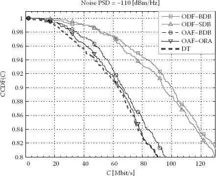
FIGURE 20.4
CCDF of achievable rate obtained using ODF and OAF with the relay located according to the best performers of the described configurations in single-sub-topology networks. The CCDF of capacity obtained assuming DT mode when no relay is connected to the network is also reported. M = 1536.

20.5.4 Power Saving with ODF and OAF

In order to assess the performance of the described ODF power allocation algorithm, we set the target rate equal to the capacity of the DT link, that is, R = C_DT when $P_{S, D T}^{(k)} = \bar{P}, \forall k \in K_{o n} .$ $P_{S, D T}^{(k)} = \bar{P}, \forall k \in K_{o n} .$ Figure 20.5 shows the cumulative distribution function (CDF) of the total transmitted power for DT and for ODF when considering the various single-sub-topology relay configurations. The noise level is set to -110 dBm/Hz. From Figure 20.5, we can see that the best relay position is the SDB. With probability equal to 0.8, it allows for saving 2.6 dB. With the same probability, the BDB relay configuration allows for saving about 1.2 dB. We have found that similar results are obtained considering the low noise level. In particular, with probability equal to 0.8, the SDB and the BDB configurations lead to a power saving of 2 and 0.9 dB.

Although not shown, we highlight that the use of OAF yields to small power savings w.r.t. DT. We could have expected this result since the achievable rate of OAF is close to that of DT (see Figure 20.4).

We now turn our attention to the network coverage (number of links satisfying the target rate) improvements that can be obtained with the use of a relay. To this end, we consider the MPM, the ORAS and the ORAD relay configurations in a two-sub-topology network. Since the S–D links experience high attenuation given by the presence of CBs in the MP, we infer that the use of the relay should yield high coverage extension. To validate our conjecture, we consider the following scenario. We impose a target rate of 100 Mbit/s, for example, as required by a multimedia application to be delivered from the living room to the bedroom located in an upper floor. In Table 20.2, we report the percentage of links that satisfy the requirements for both measured and generated channels using DT and ODF with MPM, ORAS and ORAD relay configurations. We also report the average total transmitted power. Looking at the results, we note that the use of the relay does not substantially increase the coverage when we place it in a random outlet belonging to either the source or the destination sub-topology (ORAS and ORAD configurations). Notably, when we place the relay in between the CBs of the MP (MPM configuration), for the high noise level, the coverage increases by 47% and the corresponding power saving is equal to 1.9 dB. When the noise level is low, we still have high power saving given by the use of a relay, but the gains associated to the coverage extension are reduced below 5%. This is simply explainable observing that for low noise levels, the imposed target rates are also achievable using the DT.

FIGURE 20.5
CDF of the total transmitted power using ODF with the relay located according to the various described configurations in single-sub-topology networks and the DT. M = 1536.

TABLE 20.2

Percentage of Satisfied Links and Mean Transmitted Power for Two-Sub-Topology Networks Using DT and ODF

	DT		ODF
Conf.	% of Satisfied Links	E[P_DT] (dBm)	% of Satisfied Links	E[P_ODF] (dBm)
Noise PSD = −110	(dBm/Hz)
ORAS	54.9	21.8	59.3	21.5
ORAD	55.2	21.8	59.1	21.5
MPM	52.4	22	77	20.1
Noise PSD = −140	(dBm/Hz)
ORAS	97.9	9.5	99	7.2
ORAD	97.9	9.5	98.7	7.6
MPM	97.8	9.8	99.9	2.6

Note: The rate target is 100 (Mbit/s).

Regarding the OAF, we notice that it does not bring to any appreciable power saving and/or coverage increase.

20.6 Conclusion

The use of half-duplex time division ODF and OAF relay protocols can provide achievable rate improvements, power saving and coverage extension over in-home PLC networks.

An optimal power and time slot allocation algorithm can be used to maximise the ODF achievable rate with a PSD constraint. Furthermore, a simplified algorithm that is based on the solution of two convex subproblems can be adopted to address the power minimisation problem of ODF with a target rate constraint.

Numerical results obtained considering the specific and peculiar application of the algorithms to the in-home PLC scenario show that, in general, ODF performs better than OAF. Significant rate improvements and power savings can be obtained depending on the relay position and the size of the network. In the considered single-circuit (single-sub-topology) network, with high reliability, achievable rate gains (up to 50%), or power savings (up to 3 dB), are offered by ODF when the relay is placed in the derivation box that feeds the source node or in a derivation box that lies on the backbone link between the source and the destination nodes. In the considered two-circuit network connected at the MP, for example, a typical two-floor house network, the best relay location is in the MP. Also in this case, substantial achievable rate improvements (up to 27%), power savings (up to 1.9 dB) and coverage extension (up to 47%) have been found.

References

1. IEEE Std. 802.3az. 2010. Management Parameters for Energy Efficient Ethernet. ISBN 978-0-7381-6486-1.

2. HomePlug Alliance. 2012. HomePlug Gren PHY 1.1 – The Standard for In-Home Smart Grid Powerline Communications: An application and technology overview. Version 1.02, 3 October 2012.

3. Tonello, A.M., S. D’Alessandro and L. Lampe. 2010. Cyclic prefix design and allocation in bit-loaded OFDM over power line communication channels. IEEE Trans. Commun. 58(11) (November): 3265–3276.

4. Kramer, G., I. Maric, and R. Yates. 2006. Cooperative Communications. Hanover, MA: NOW Publishers Inc.; Found. Trends Networking 1(3): 271–425.

5. Host-Madsen, A. and J. Zhang. 2005. Capacity bounds and power allocation for the wireless relay channel. IEEE Trans. Inf. Theory 51(6) (June): 2020–2040.

6. Gündüz, D. and E. Erkip. 2007. Opportunistic cooperation by dynamic resource allocation. IEEE Trans. Wireless Commun. 6(4) (April): 1446–1454.

7. Xie, L. and X. Zhang. 2007. TDMA and FDMA based resource allocations for quality of service provisioning over wireless relay networks. In Proceedings of the IEEE Wireless Communication and Networking Conference, Hong-Kong, China, pp. 3153–3157.

8. Hammerström,, I. and A. Wittneben. 2006. On the optimal power allocation for nonregenerative OFDM relay links. In Proceedings of the IEEE International Conference on Communications, Istanbul, Turkey, vol. 10, June 2006, pp. 4463–4468.

9. Zhang, W., U. Mitra and M. Chiang. 2011. Optimization of amplify-and-forward multicarrier two-hop transmission. IEEE Trans. Commun. 59(5): 1434–1445.

10. Li, X., J. Zhang and J. Huang. 2009a. Power allocation for OFDM based links in hybrid forward relay. In Proceedings of the IEEE Vehicular Technology Conference, Barcelona, Spain, April 2009.

11. Li, Y., W. Wang, J. Kong and M. Peng. 2009b. Subcarrier pairing for amplify-and-forward and decode-and-forward OFDM-relay links. IEEE Commun. Lett. 13(4): 209–211.

12. Ying, W., Q. Xin-Chun, W. Tong and L. Bao-Ling. 2007. Power allocation subcarrier pairing algorithm for regenerative OFDM relay system. In Proceedings of the IEEE Vehicular Technology Conference, Dublin, Ireland, April 2007, pp. 2727–2731.

13. Liang, Y., V. Veeravalli and V. Poor. 2007. Resource allocation for wireless fading relay channels: Max-min solution. IEEE Trans. Inf. Theory 53(10): 3432–3453.

14. Gesbert, D., S. Hanly, H. Huang, S. Shamai-Shitz and W. Yu. 2010. Guest editorial: Cooperative communications in MIMO cellular networks. IEEE J. Sel. Areas Commun. 28(9): 1377–1379.

15. Bakanoglu, K., S. Tomasin and E. Erkip. 2011. Resource allocation for the parallel relay channel with multiple relays. IEEE Trans. Wireless Commun. 10(3): 792–802.

16. Bumiller, G. 2002. Single frequency network technology for medium access and network management. In Proceedings of the IEEE International Symposium on Power Line Communications and Its Applications, Athens, Greece, March 2002.

17. Bumiller, G., L. Lampe and H. Hrasnica. 2010. Power line communication networks for large-scale control and automation systems. IEEE Commun. Mag. 48(4): 106–113.

18. Lampe, L., R. Shober and S. Yiu. 2006. Distributed space-time block coding for multihop transmission in power line communication networks. IEEE J. Sel. Areas Commun. 24(7): 1389–1400.

19. Biagi, M. and L. Lampe. 2010. Location assisted routing techniques for power line communications in smart grids. In Proceedings of the IEEE International Conference on Smart Grid Communications, Gaithersburg, MD, October 2010, pp. 274–278.

20. Biagi, M., S. Greco and L. Lampe. 2012. Neighborhood-knowledge based geo-routing in PLC. In Proceedings of the IEEE International Symposium on Power Line Communications and Its Applications, Beijing, China, April 2012, pp. 7–12.

21. Lampe, L. and A.J.H. Vinck. 2012. Cooperative multihop power line communications. In Proceedings of the IEEE International Symposium on Power Line Communications and Its Applications, Beijing, China, March 2012, pp. 1–6.

22. Zou, H., A. Chowdhery, S. Jagannathan, J. M. Cioffi and J.L. Masson. 2009. Multi-user joint sub-channel and power resource-allocation for powerline relay networks. In Proceedings of the IEEE International Conference on Communications, Dresden, Germany, June 2009.

23. Tan, B. and J. Thompson. 2011a. Relay transmission protocols for in-door powerline communications networks. In Proceedings of the IEEE International Conference on Communications, Kyoto, Japan, June 2011, pp. 1–5.

24. Tan, B. and J. Thompson. 2011b. Capacity evaluation with channel estimation error for the decode-and-forward relay PLC networks. In Proceedings of the European Signal Processing Conference, Barcelona, Spain, August 29–September 2, 2011, pp. 834–838.

25. Tlich, M., R. Razafferson, G. Avril and A. Zeddam. 2008. Outline about the EMC properties and throughputs of the PLC systems up to 100 MHz. In Proceedings of the IEEE International Symposium on Power Line Communications and Its Applications, Jeju Island, Korea, April 2008, pp. 259–262.

26. Cover, T.M. and J.A. Thomas. 2006. Elements of Information Theory. New York: Wiley & Sons.

27. Bumiller, G. 2012. Transmit signal design for NB-PLC. In Proceedings of the IEEE International Symposium on Power Line Communications and Its Applications, Beijing, China, March 2012, pp. 132–137.

28. D’Alessandro, S., A. M. Tonello and L. Lampe. 2011. Adaptive pulse-shaped OFDM with application to in-home power line communications. Springer Telecommun. Syst. J. 50: 1–11.

29. Comitato Elettrotecnico Italiano (CEI). 2007. Norma CEI per impianti elettrici utilizzatori – CEI norm for electrical systems. Milan, Italy: CEI, 2007.

30. Tonello, A.M. and F. Versolatto. 2010. Bottom-up statistical PLC channel modeling – Part II: Inferring the statistics. IEEE Trans. Power Delivery 25(4): 2356–2363.

31. Latchman, H. and R. Newman. 2007. HomePlug standards for worldwide multimedia inhome networking and broadband powerline access. In International Symposium on Power Line Communications and Its Applications, Speech II, Pisa, Italy. http://www.ieee-isplc.org/2007/docs/keynotes/latchman-newman.pdf (accessed September 23, 2012).

32. Campello, J. 1999. Practical bit loading for DMT, In Proceedings of the IEEE International Conference on Communications (ICC ‘99), Vancouver, Canada, June 1999, vol. 2, pp. 801–805.

33. Hanly, S. and D. Tse. 1998. Multiaccess fading channels – Part II: Delay-limited capacities. IEEE Trans. Inf. Theory. 44(7): 2816–2831.

34. Papandreou, N. and T. Antonakopoulos. 2008. Bit and power allocation in constrained multicarrier systems: The single-user case. EURASIP J. Adv. Signal Process. Article ID 643081: 2008: 1–15.

35. Cui, S., R. Madan, A. Goldsmith and S. Lall. 2005. Energy-delay tradeoffs for data collection in TDMA-based sensor networks. In Proceedings of the IEEE International Conference on Communications, Seoul, South Korea, pp. 3278–3284.

36. Boyd, S. and L. Vandenberghe. 2004. Convex Optimization. Cambridge, MA: Cambridge University Press.

37. Kuhn, H.W. and A.W. Tucker. 1951. Nonlinear programming. In Proceedings of Second Berkeley Symposium on Mathematical Statistics and Probability, California, Berkeley, CA, August 1951, pp. 481–492.

38. Weisstein, E.W. Sylvester’s criterion. http://mathworld.wolfram.com/SylvestersCriterion.html (accessed September 23, 2012).

39. D’Alessandro, S. and A.M. Tonello. 2012. On rate improvements and power saving with opportunistic relaying in home power line networks. EURASIP J. Adv. Signal Process. 194: 1–16.

40. Afkhamie, K., S. Katar, L. Yonge and R. Newman. 2005. An overview of the upcoming HomePlug AV Standard. In Proceedings of the IEEE International Symposium on Power Line Communications and Its Applications, Vancouver, British Columbia, Canada, April 2005, pp. 400–404

41. CENELEC. 2012. Final Draft of EN-50561-1 Standard. Power line communication apparatus used in low-voltage installations – Radio disturbance characteristics – Limits and methods of measurement – Part 1: Apparatus for in-home use. Brussels, Belgium: CENELEC, 2012.

42. Tonello, A.M. and F. Versolatto. 2010. Bottom-up statistical PLC channel modeling – Part I: Random topology model and efficient transfer function computation. IEEE Trans. Power Delivery 26(2): 891–898.

43. Versolatto, F. and A.M. Tonello. 2012. On the relation between geometrical distance and channel statistics in in-home PLC networks. In Proceedings of the IEEE International Symposium on Power Line Communications and Its Applications, Beijing, China, March 2012, pp. 280–285.

44. Ferreira, H.C., L. Lampe, J. Newbury and T.G. Swart. 2010. Power Line Communications: Theory and Applications for Narrowband and Broadband Communications over Power Lines. New York: Wiley & Sons.

45. Laneman, J., D. Tse and G. Wornell. 2004. Cooperative diversity in wireless networks: Efficient protocols and outage behavior. IEEE Trans. Inf. Theory 50(12): 3062–3080.

*. The assumption on the transmitted symbols to be i.i.d. Gaussian distributed is meant to compute the capacity, that is, the maximum achievable rate (Cover and Thomas 2006).

..................Content has been hidden....................

You can't read the all page of ebook, please click here login for view all page.

Table of Contents for 20. Relaying Protocols for In-Home PLC

Create new playlist

Sign In

Sign Up

Table of Contents for
20. Relaying Protocols for In-Home PLC