Radiation Mitigation for Power Line Communications Using Time Reversal*
Contens
17.2 Time Reversal for Power Line Communications
17.2.1 Time Reversal for Wireless Transmission
17.2.2 Extension of Time Reversal to Wired Transmission
17.4 Results and Statistical Analysis
17.4.2 Statistical Analysis of the Time Domain Measurements
17.5 Concept Validation on Frequency Domain Measurements
17.5.1 Frequency Domain Measurements Database
17.5.2 Statistical Analysis of the Frequency Domain Measurements
With the increasing demand for both high data rate applications and reliable links for command and control systems, power line communication (PLC) has emerged in recent years as an attractive communication technique [2]. The main advantage of this technology is its ability to benefit from the existing electrical network infrastructure for the transmission of electromagnetic signals. Hence, it becomes possible to build large communication networks without the need for installing new wires.
In the home or office environment, indoor PLC uses the low-voltage (LV) infrastructure. The presence of several electrical outlets in each room of the house allows ubiquitous coverage of the communication network. In addition, the relatively short distance between different outlets allows the system to operate within a limited attenuation. Current broadband (BB) inhome systems primarily operate in the frequency range from 2 to 30 MHz. However, recent specifications, such as IEEE 1901 [3] or ITU-T G.9960 [4], allow signal transmission at higher frequencies up to 100 MHz. On the other hand, narrowband (NB) PLC systems are deployed at frequencies below 500 kHz, in both indoor and outdoor configurations, using LV or medium-voltage (MV) infrastructures [5]. These systems allow the transmission of command and control information over longer distances for Smart Grid applications. The ITU-T G.9955 standard is an example of such NB PLC systems [6]. More information on current NB and BB PLC systems is given in Chapter 10 and subsequent chapters.
LV or MV electrical wires were not initially designed to propagate communication signals at frequencies above 1 kHz. As a consequence, the communication channel between the transmitter (Tx) and the receiver (Rx) is a difficult channel, generating attenuation and multiple propagation paths. The channel capacity is, hence, limited, and signal processing needs to be optimised so as to maximise the offered data rate and quality of service (QoS).
This chapter focuses on one of the main limitations related to the PLC technology, namely, the generation of unintentional radiated signal. This phenomenon is mainly due to the unbalanced nature of the electrical network [7]. The variation of the impedances of the loads connected to the network as well as the unequal length of the live and neutral wires (due to single-phase switches) converts the differential PLC signal into common-mode current flowing through the network. Consequently, the copper wires used for transmitting the useful signal act as an antenna, and part of the transmitted power is radiated. This not only results in stronger signal attenuation at the Rx but also leads to electromagnetic compatibility (EMC) issues, as the radiated signal may interfere with other existing services, such as amateur radio (HAM) or short-wave (SW) broadcasting. The impact of PLC transmission on EMC has been studied, for example, within the ICT FP7 project OMEGA [8] and through the ETSI Specialist Task Force 410 [9]. Chapter 7 presents a detailed study of the EMC impact of PLC based on a series of field measurements.
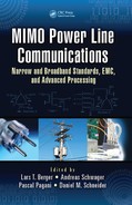
In order to avoid interference between PLC systems and other users of the spectrum, regulation authorities impose strict emission masks for the transmission of electromagnetic signals on the power lines. In the United States, the Federal Communications Commission (FCC) Part 15 [10] specifies a maximum level of radiated field for carrier-current systems (including PLC), leading system specifications to define constrained power transmission masks. Figure 17.1 represents an example of power spectral density (PSD) limits provided in the IEEE 1901 standard for North America. The observed notches are defined to protect specific systems, such as HAM bands. In Europe, CENELEC is currently developing a draft regulation standard applying to in-home PLC systems [11]. Chapter 6 discusses the current regulation status for both NB and BB PLC systems.
Regardless of the regulation limits in place, the research presented in this chapter focuses on the mitigation of unintentional radiation due to PLC systems. Several attempts to solve this problem have been presented in the literature. Reference [12] presents a method to reduce radiated emissions by applying an auxiliary signal cancelling the electromagnetic field on a given point in space. Simulations demonstrated good performance, with the drawback that the electromagnetic interference (EMI) could only be mitigated at a single location. The authors in Ref. [13] used additional hardware connected at the wall outlets, in order to reduce asymmetries on power lines, at the cost of an increased complexity of the PLC network.
The presented approach tries to simultaneously reach two complementary goals by means of digital signal processing. The first intention is to focus the transmitted signal at the Rx location. The power gain linked to this energy focalisation allows in turn relaxing the required power level at the Tx, hence generating less EMI. A second target is to reduce the level of energy dissipated at any location except the intended Rx. In particular, it is desirable to minimise the level of radiated power from the electrical wires. These two benefits already appear as features of a known technique in the field of wireless transmission: time reversal (TR) [14]. Experimental investigations conducted using ultra-wideband (UWB) radio waves demonstrated both the focusing and interference mitigation properties of this technique [15,16].
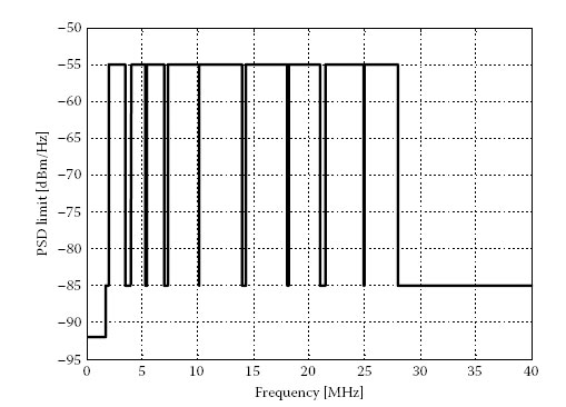
FIGURE 17.1
Example of PSD limit for North America. (From Mescco, A. et al., Hindawi J. Electr. Comput. Eng., 2013, Article ID 402514, Copyright © 2013.)
This chapter presents an experimental analysis of TR as a means to mitigate radiation effects for wired signal transmission. Our investigation focuses on high-frequency (HF) BB PLC signals but could be extended to NB PLC and other wired transmission systems, such as digital subscriber line (DSL) access. The chapter is organised as follows. Section 17.2 presents the concepts of the TR technique and its application to wired systems. Section 17.3 details the experiment conducted to assess the merits of TR for BB PLC, and the results are statistically analysed in Section 17.4. Section 17.5 validates the concept on the basis of frequency domain measurements. Finally, conclusions are drawn in Section 17.6.
17.2 Time Reversal for Power Line Communications
17.2.1 Time Reversal for Wireless Transmission
The TR technique, also known as phase conjugation in the frequency domain, was first used in the fields of acoustics [17,18]. More recently, this concept has been successfully extended to electromagnetic waves, where the rich multipath channel provides excellent conditions for its application [14]. The basic concept of TR is simple. Let δ(τ) be an ideal, Dirac impulse emitted by a Tx antenna (Figure 17.2a). By definition, at any Rx location r0, the received signal is given by the channel impulse response (CIR) h(τ, r0). The CIR is composed of multiple echoes reflecting the multiple propagation paths of the propagation channel.

FIGURE 17.2
Transmission over an ideal multipath propagation channel: (a) of a Dirac impulse and (b) of the time reversed CIR. (From Mescco, A. et al., Hindawi J. Electr. Comput. Eng., 2013, Article ID 402514, Copyright © 2013.)
TR uses this channel state information (CSI) at the Tx to prefilter the signal to be transmitted. More specifically, the CIR h(τ, r0) is time reversed and normalised to serve as an input filter for the signal to be transmitted (Figure 17.2b). Physically, each delayed echo constituting the TR filter travels, among other multiple paths, through its original propagation path. As a result, the multiple echoes sum up coherently at the Rx, hence focusing the received energy in time.
Mathematically, applying TR leads for any Rx situated at an arbitrary location r to the equivalent perceived CIR hTR(τ, r) (note that this formulation holds for a real valued CIR) [19]:
(17.1) |
where the symbol ⊗ denotes time domain convolution. Formulating Equation 17.1 in the frequency domain leads to
(17.2) |
where
H(f, r) represents the complex valued channel transfer function (CTF)
the superscript* denotes the complex conjugate operation
For this reason, TR is sometimes called frequency domain phase conjugation.
Two conclusions can be drawn from Equations 17.1 and 17.2. First, at the intended Rx location r0, the perceived CIR simplifies to
(17.3) |
where rh(τ, r0) denotes the time domain autocorrelation of the function h(τ, r0). Similarly, the perceived CTF simplifies to
(17.4) |
In the time domain, the effect of the TR filter is to transform the CIR into its autocorrelation. For a rich multipath environment, the autocorrelation of the CIR presents a large peak at τ = 0, with reduced side echoes. Experimental studies demonstrated that the resulting channel is less spread in time [15,16], hence reducing the possible intersymbol interference (ISI). In the frequency domain, the perceived CTF is proportional to the square of the magnitude of the actual CTF. Besides the fact that TR provides a real valued CTF, which could be exploited at the Rx, this also leads to a significant gain in terms of Rx power, due to a better exploitation of the frequency selective nature of the channel. It was demonstrated in Ref. [19] that the application of TR in a flat channel (i. e. without frequency domain power decay) under Rayleigh fading leads to a gain of 3 dB in the total received power. This gain was increased to 5 dB when considering the frequency domain power decay observed in practical UWB radio channels.
The second conclusion drawn from Equations 17.1 and 17.2 is that for any other location r different from r0, TR creates a mismatch between the Tx filter and the channel. This is particularly observable in the frequency domain representation of TR given in Equation 17.2. The perceived CTF corresponds to the product of two independent CTF, H(f, r) and H*(f, r0), with possibly very different frequency-fading structures. More precisely, minima of the first CTF can happen randomly at maxima of the second CTF. Hence, averaging over all frequencies, the total received power at untargeted locations is reduced. In wireless TR analysis, this effect is called spatial focusing and is generally assessed as the ratio between the maximum of hTR(τ, r) and the maximum of hTR (τ, r0) for a given distance . Spatial focusing factors of −10 dB have been reported in Refs. [19,20].
17.2.2 Extension of Time Reversal to Wired Transmission
As observed through the study of TR for wireless transmission, the TR scheme provides two main features, namely, an increase of the Rx power at the intended Rx location and a decrease of the Rx power at any other location. These features are highly desirable in the context of wired transmission, where the level of Tx power is constrained by the unintentional radiation from the wires, causing possible EMI to other systems.
Based on this observation, experimental studies were conducted to analyse the potential of TR to mitigate unwanted emissions for PLC systems. The main principles of the extension of TR to PLC transmission can be explained with the help of Figure 17.3.
An intended transmission is assumed between a Tx PLC modem and an Rx PLC modem, over a LV indoor electrical network. Different experimental investigations reported the PLC channel as a rich multipath propagation channel, due to the multiple branches present in a classical electrical network and to the impedance mismatch occurring at the network terminations (outlets) and nodes [21–24]. This similarity of the PLC channel with wireless channels suggests promising results when applying TR to PLC.
With reference to Figure 17.3, the Rx modem is situated at the intended location r0, and the Tx modem is situated at the origin. By applying TR filtering at the Tx, the Rx power will be increased at location r0; hence, the Rx modem will benefit from an increased signal-to-noise ratio (SNR). This power increase can also in turn be applied as a reduction of the Tx power to achieve similar performance. At other outlets in the network, situated, for example, at locations r1 or r2, the Rx power will be reduced. This effect can be further exploited in the design of multi-user transmission schemes.
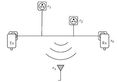
FIGURE 17.3
Principle of the extension of TR to wired transmission. (From Mescco, A. et al., Hindawi J. Electr. Comput. Eng., 2013, Article ID 402514, Copyright © 2013.)
For our purpose of radiation mitigation, let us now consider a location r3, situated at any point in space in the vicinity of the electrical network. The level of radiated field at this location can be evaluated, for instance, by means of an equivalent transfer function H(f, r3) between the Tx modem and an ideal antenna situated at location r3. By the virtue of the TR scheme (Equation 17.2), the perceived transfer function at location r3 after applying TR will be proportional to the product . As the functions H*(f, r0) and H(f, r3) are not correlated, their frequency fading structures are different. In particular, the deep notches due to frequency-selective fading do not appear at the same frequencies. As a result, the product will provide more average attenuation when compared to H(f, r3) alone, and therefore, the total power radiated at location r3 will be reduced. A similar observation is made in previous studies dedicated to wireless channels [14,15,18]. Hence, TR appears as an efficient method to mitigate EMI for wired communications.
The theoretical basis for the application of TR to wired transmission being set, the experimental assessment of this method will be described in the next sections.
In order to experimentally assess the use of TR as a method to mitigate EMI for wired communication, the experimental setup presented in Figure 17.4 was used. In this setup, a signal generator Tektronix AWG7082C was used as a generic Tx. A digital sampling oscilloscope (DSO) LeCroy WaveRunner 715Zi-A was used to sample the received signal at Rx. The signal generated at Tx is denoted s(t), and the signal received at the DSO is denoted y(t). Two universal PLC couplers were used as baluns to couple the Tx and Rx signals with the power lines. The Tx coupler is situated at the origin, and the Rx coupler is connected to a plug at location r0. These couplers were developed within the ETSI Specialist Task Force 410 [25]. In order to measure the power density of the radiated emission received at any arbitrary location r3, a biconical antenna Schwarzbeck EFS921 was connected to a second port of the DSO.
FIGURE 17.4
Equipment used in the experimental setup. (From Mescco, A. et al., Hindawi J. Electr. Comput. Eng., 2013, Article ID 402514, Copyright © 2013.)
With reference to Figure 17.5, two measurement paths cans be distinguished. Path 1 serves for the measurement of the CTF and is composed of the following elements: the Tx, coaxial cable 1, a 30 dB amplifier IFIM50, coaxial cable 2, balun 1, mains, balun 2, coaxial cable 3, a 20 dB attenuator Radial R412720000 and the Rx. The baluns were considered as part of the channel. The calibration for measurement path 1 was made by directly connecting coaxial cable 2 and coaxial cable 3.
Path 2 is composed by the Tx, coaxial cable 1, a 30 dB amplifier IFIM50, coaxial cable 2, the wire to free space propagation channel (represented by the CTF H(f, r3)), the biconical antenna, coaxial cable 4 and the DSO. The calibration for this second path was made by connecting coaxial cable 2 and coaxial cable 4. The gain of the antenna was removed from the measurements by postprocessing.
The signal generator and the DSO were synchronised by a direct connection of their 10 MHz reference clocks. The sampling rates of both devices were set to fs = 100 MHz.
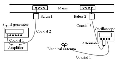
FIGURE 17.5
Experimental setup calibration. (From Mescco, A. et al., Hindawi J. Electr. Comput. Eng., 2013, Article ID 402514, Copyright © 2013.)
After initial system calibration, the measurements are performed in three steps:
1. The CTF H(f, r0) is evaluated using a specific Tx frame (see succeeding text). The considered frequency band extends from 2.8 to 37.5 MHz.
2. The TR filter is generated using the phase and magnitude of H(f, r0).
3. The CTFs H(f, r0) and H(f, r3) as well as the perceived CTFs HTR(f, r0) and HTR(f, r3) are measured using a single Tx frame (see succeeding text). Measurements at the location of the Rx outlet (r0) and at arbitrary locations in space (r3) are made simultaneously using two ports of the oscilloscope, one connected to the Rx balun and the other connected to the biconical antenna.
The Tx signal is generated according to the HomePlug standard [26]. The used frame is called PHY protocol data unit (PPDU), and it is composed by a preamble (including a frame control) and a number of payload symbols as shown in Figure 17.6. Each payload symbol consists of a 3072-sample orthogonal frequency division multiplexing (OFDM) symbol as defined in the HomePlug specification [26]. In order to estimate the CTFs H(f, r) and HTR(f, r), the OFDM symbols were loaded with predefined constellations.
The frame used for the calibration and the initial measurement of the CTF before computation of the TR filter is represented in Figure 17.7.
The frame used for the measurement of the CTF and EMI after computation of the TR filter is represented in Figure 17.8. Note that in this frame, the TR filter is applied on the last three symbols only (represented by the signal s′(t)). From this particular frame scheme, the CTF and EMI can be evaluated with and without application of TR quasi-simultaneously. Recomputing the CTF at this stage also allows monitoring any possible temporal evolution of the channel between calibration and measurement.
In essence, the overall channel estimation process is similar to the channel sounding procedure defined in the HomePlug AV specification. In our experiment, the computation of the CTF from the received signal uses a classical zero-forcing (ZF) channel estimation procedure. This is suitable in our experiment involving high levels of SNR at the Rx. In practical systems operating at lower SNR, more sophisticated methods such as the minimum mean square error channel estimation would be more efficient against noise enhancement. Note that the TR filter was purposely implemented in the time domain at the Tx using a programmable waveform generator, in order to measure results as close as possible to a realistic implementation of the TR scheme in practical PLC modems.

FIGURE 17.6
HomePlug frame. (From Mescco, A. et al., Hindawi J. Electr. Comput. Eng., 2013, Article ID 402514, Copyright © 2013.)

FIGURE 17.7
HomePlug frame for calibration and CTF measurement before computation of the TR filter. (From Mescco, A et al., Hindawi J. Electr. Comput. Eng., 2013, Article ID 402514, Copyright © 2013.)

FIGURE 17.8
HomePlug frame for CTF and EMI measurement after application of TR. (From Mescco, A. et al., Hindawi J. Electr. Comput. Eng., 2013, Article ID 402514, Copyright © 2013.)
In order to estimate channel attenuation continuously over the measured frequency band, no spectral notches were implemented for this study. In practical systems, a Tx PSD mask is defined, where the Tx power is notched at predefined frequencies, to protect existing services using the same spectrum. The HomePlug specification uses windowing in order to better exploit the power allocated within the PSD mask while protecting out-of-band services. The present study concentrates on reducing the EMI within the band effectively used by PLC systems. Therefore, the results also hold for practical systems including notches.
The measurement campaign was conducted using 13 different topologies of 230 V mains networks within the premises of Orange Labs in Lannion. The campaign took place in different rooms of about 5 × 4 m2. Figure 17.9 presents a picture of the experimental setup in an exemplar location.
The Tx and Rx modems were connected to two outlets in the same room, with distances varying between 2 and 8 m. In general, the rooms are equipped with several other electrical outlets (between 4 and 10). About half of the outlets were connected to classical office appliances (lamps, desktops, etc.). For each topology, one CTF was measured, first without applying TR and then after applying TR filtering. In addition, for each topology, between three and five locations were selected to measure the received electrical field with the help of the biconical antenna. In total, 13 CTF and 43 measurements of the electrical field were collected for statistical analysis.

FIGURE 17.9
Picture of experimentation. (From Mescco, A. et al., Hindawi J. Electr. Comput. Eng., 2013, Article ID 402514, Copyright © 2013.)
17.4 Results and Statistical Analysis
The preliminary results for an exemplar network will be presented in two parts: first, the CTF at r0 and, second, the electrical field and its associated power density at r3 ≠ r0.
The attenuation characteristics of the CTF at r0 are shown in Figure 17.10.
Let us first consider the measured CTF (solid line). The deep notches at some frequencies are due to reflections at the terminations of the network and reflect the multipath nature of the PLC network. The average attenuation before TR is defined in dB as follows:
(17.5) |
where fmin and fmax, respectively, represent the minimum and maximum sounded frequencies. The average attenuation corresponds to the signal attenuation perceived by an Rx capable of exploiting all the power received in the frequency band from fmin to fmax. Typically, an OFDM system like the HomePlug AV specification is able to exploit the total received power over a wide frequency band. In our example, the average attenuation is about 11 dB.
Let us now focus on the perceived CTF after applying TR. Owing to the mathematical definition of the TR filter, TR allocates more power to frequencies showing minimal attenuation, while strongly attenuated frequencies are more power constrained. In particular, for all frequencies where the attenuation of the channel H(f, r0) is higher than the average attenuation , the perceived channel is more attenuated after applying TR. This can be clearly seen in the frequency range from 26 to 37.5 MHz. For the frequencies where the attenuation of the channel is less than , the response of the channel is improved using TR. This is clearly observable in the frequency range from 11 to 22 MHz. Defining the average attenuation after TR in dB as

FIGURE 17.10
Channel attenuation before and after TR. (From Mescco, A. et al., Hindawi J. Electr. Comput. Eng., 2013, Article ID 402514, Copyright © 2013.)
(17.6) |
it can be observed that the average attenuation after applying TR is about 7.5 dB. Hence, the application of TR provided a gain in the total received power of 3.5 dB in this particular example.
Note that only the measured CTF (solid line) is physical. Therefore, the measured CTF will always degrade the transmission with some degree of channel attenuation. On the contrary, the CTF perceived at Rx after application of TR (dashed line) corresponds to a logical channel, where the effects of the measured CTF are combined with the effects of the TR filter at Tx. Hence, the perceived CTF may exhibit some gain over a limited frequency range.
Let us now consider the electrical field and its associated power density at r3 ≠ r0. The value of the electrical field E(f, r3) in dBμV/m was computed from the CTF H(f, r3) measured between the Tx balun and the antenna connector assuming an injected PSD Pfeed = −55 dBm/Hz, and using the following formula [25]:
(17.7) |
where
AF(f) represents the antenna factor
107 represents the conversion from dBm to dBμV
In addition, the average radiated power density was computed in dB (W/m2) as follows:
(17.8) |
where
fmin and fmax, respectively, represent the minimum and maximum sounded frequencies E(f, r3) is expressed in V/m
In Equation 17.8, the term 120π provides the value of the impedance of free space in Ohm.
Note that both E(f, r3) and can also be computed after applying TR filtering, using the following equations:
(17.9) |
and
(17.10) |

FIGURE 17.11
Electrical field before and after TR. (From Mescco, A. et al., Hindawi J. Electr. Comput. Eng., 2013, Article ID 402514, Copyright © 2013.)
An example of radiated emission measurement is given in Figure 17.11. For this particular electrical network, the mitigation of radiated emissions is clear in the frequency band from 26 to 37.5 MHz, and the average radiated power density has reduced by about 7.5 dB. Thus, it can be observed with this example that the application of TR filtering can reduce significantly the level of undesired radiated power.
17.4.2 Statistical Analysis of the Time Domain Measurements
This section presents the statistical analysis of the measurement database collected within 13 rooms of the office building at Orange Labs in Lannion. The total measurement set is composed of 13 CTF and 43 measurements of the electrical field.
The channel gain GTR observed on the perceived CTF HTR(f, r0) after application of TR filtering is first computed. As OFDM systems can exploit the total power received over a given frequency band, this gain is computed in dB for the total received power as
(17.11) |
The cumulative distribution function (CDF) of GTR is given in Figure 17.12. This parameter shows always a positive gain, between 1.4 and 6.6 dB in our experiment, which is in line with results reported in similar wireless experiments [19]. In about 60% of cases, the channel gain is higher than 3 dB. This means that at Rx, there is always a better reception using TR. This channel gain can in turn be used to reduce the injected PSD at Tx, hence reducing by the same factor the unwanted EMI.
The EMI reduction coefficient RTR was then computed, corresponding to the reduction of the undesired radiated power due to the application of a TR filter. This figure of merit of the reduction of radiated signal is computed in dB as follows:
(17.12) |
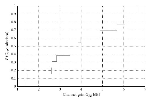
FIGURE 17.12
CDF of the channel gain GTR for the time domain experiment. (From Mescco, A. et al., Hindawi J. Electr. Comput. Eng, 2013, Article ID 402514, Copyright © 2013.)
The CDF of the EMI reduction coefficient RTR is given in Figure 17.13. Results show that the simple application of TR reduces the EMI in more than 60% of cases. In the best case, the EMI reduced by more than 7 dB using TR. In the worst case, the EMI increased by 2 dB. The observations of particular cases indicates that the reduction of EMI is more effective when the CTFs H(f, r0) and H(f, r3) are highly decorrelated. This is more likely to happen in complex electrical network topologies, where the rich multipath environment results in different frequency fading structures for different Rx locations.
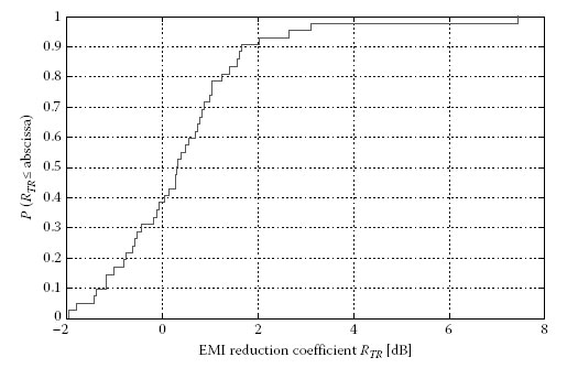
FIGURE 17.13
CDF of the EMI reduction coefficient RTR for the time domain experiment. (From Mescco, A. et al., Hindawi J. Electr. Comput. Eng., 2013, Article ID 402514, Copyright © 2013.)
Observing the statistics of the channel gain GTR and of the EMI reduction coefficient RTR, an optimal strategy can be proposed in order to minimise EMI for a PLC system. Indeed, Figure 17.12 shows that the application of TR provides better system performance due to the reduced channel attenuation. This gives us in turn the flexibility to reduce the level of the Tx power to further reduce EMI while keeping the system performance constant. More precisely, when TR is applied, a Tx power backoff of GTR dB can be applied without modifying the total received power. Finally, following this power backoff strategy, the effective EMI mitigation factor MTR can be computed as the sum of the power backoff and the EMI reduction coefficient:
(17.13) |
The CDF of the effective EMI mitigation factor MTR is depicted in Figure 17.14. Several conclusions can be drawn from this statistical result:
1. First, the TR method is able to mitigate EMI generated by PLC transmission in 100% of our experimental observations. To this respect, one can conclude that the gain GTR provided by the application of TR allows a Tx power backoff that largely compensates for the possible EMI increment observed in Figure 17.13.
2. Second, in 40% of the cases, the undesired radiated power is reduced by more than 3 dB.
3. Finally, in the most favourable configurations, a reduction of the EMI by more than 10 dB can be observed. Such configurations correspond to cases where the CTF between the Tx and Rx modem and the EMI spectrum are particularly decorrelated.

FIGURE 17.14
CDF of the effective EMI mitigation, MTR, for the time domain experiment. (From Mescco, A. et al., Hindawi J. Electr. Comput. Eng., 2013, Article ID 402514, Copyright © 2013.)
17.5 Concept Validation on Frequency Domain Measurements
17.5.1 Frequency Domain Measurements Database
In order to validate the gain of the TR technique in terms of mitigation of the radiation of PLC systems, a larger set of measurements was considered. This data set was collected in nine houses and flats located in France and Germany, in the framework of the ETSI STF 410 measurement campaign [9]. Measurements were recorded using a vector network analyser (VNA).
The PLC CTF H(f, r0) was first recorded between a Tx modem and an Rx modem, at random outlet locations in the house. In a second step, the CTF H(f, r3) between the Tx modem and an antenna situated at an arbitrary location r3 was recorded. The small biconical antenna used for this purpose allowed an easy placement at different locations within the house or outside the building. Outdoor measurement locations were selected either at 3 m or at 10 m from the external wall. In total, 114 couples of CTFs H(f, r0) and H(f, r3) were available for processing the statistical analysis. For the purpose of comparison with the results obtained in the time domain experiment, the same frequency band extending from 2.8 to 37.5 MHz was considered in the computations.
More details on the ETSI STF 410 measurement campaign and on the resulting analysis of channel, noise characteristics can be found in Chapter 5. In addition, a study of the EMI properties of the PLC channel based on this measurement campaign is provided in Chapter 7.
17.5.2 Statistical Analysis of the Frequency Domain Measurements
The first analysis consisted of studying the channel gain GTR observed on the perceived CTF HTR(f, r0) after application of the TR filter, see Equation 17.11. Figure 17.15 presents the CDF of this parameter over the whole measurement campaign. On this larger data set, the channel gain GTR of the TR technique is always greater than 0.9 dB and can be as high as 15.6 dB. About 95% of the channels present a gain larger than 3 dB and 70% of the channels present a gain larger than 6 dB.

FIGURE 17.15
CDF of the channel gain GTR for the frequency domain experiment.

FIGURE 17.16
CDF of the EMI reduction coefficient RTR for the frequency domain experiment.
The second characteristic related to the application of TR is the EMI reduction coefficient RTR, as defined in Equation 17.12. The CDF of this parameter for the frequency domain campaign is presented in Figure 17.16. One can observe that in 55% of the cases, the total power density is reduced by the TR technique, up to a maximum of 8 dB. However, in 45% of the observations, the EMI is actually increased, with a maximal increase of 5 dB. Hence, a similar trend as for the time domain experiment is observed, with larger extreme values.
The statistics presented in Figure 17.16 tend to show that in a large number of cases, the EMI is actually increased by the application of TR. However, one has to note that in the same time, the total power received at the Rx modem is significantly increased, due to the TR channel gain. Again, the optimal strategy thus consists in reducing the Tx power by GTR dB. This smart power backoff allows further reducing the EMI while preserving the power level observed at Rx, and hence keeping the same system performance. The final EMI reduction is then given by the EMI mitigation factor MTR defined in Equation 17.13. The CDF of parameter MTR for the frequency domain measurements is presented in Figure 17.17. In 98% of the cases, the resulting EMI is decreased, with a maximal reduction of 16.4 dB. Therefore, the good performance of the TR technique is confirmed on this larger data set collected in the frequency domain. One needs to note that in only 2% of the observations, the EMI is actually increased, up to a maximum of 1 dB. Further research will focus on the detection of such cases in order to avoid application of TR if it results in higher radiation.
This chapter proposed the application of TR in order to mitigate EMI generated by wired communication systems. TR was originally used in the field of wireless transmission as a mean to focus the transmitted signal in both time and space around the intended Rx. It is proposed to use the same property to focus the signal injected in a wired medium, such as the electrical network in the case of PLC, for instance. As a result, the energy lost through undesired radiation is expected to decrease significantly.

FIGURE 17.17
CDF of the effective EMI mitigation, MTR, for the frequency domain experiment.
An experimental setup was presented in order to demonstrate this method. The experiment was conducted in the time domain using signal frames similar to the industrial specification HomePlug AV. In addition, the TR filter was actually implemented using an arbitrary wave generator, thus providing results encompassing the possible drawbacks of a practical implementation.
Results demonstrated that on the wired medium, TR could provide a transmission channel gain between 1 and 7 dB, which is similar to the gain observed in wireless transmission. In addition, the application of a TR filter alone could effectively reduce EMI for 60% of the observations, with a maximum EMI mitigation of 7 dB. Finally, by combining the channel gain and the EMI reduction features, it was experimentally demonstrated that TR was efficient in 100% of the observed cases to reduce EMI. In 40% of the cases, the EMI mitigation was larger than 3 dB, with maxima higher than 10 dB. These encouraging results were confirmed by a second statistical analysis performed on a larger set of measurements conducted in the frequency domain. These measurements were collected in France and Germany in the framework of the ETSI STF 410 campaign. This second statistical study confirmed the observed trends, with larger extreme values. First, TR channel gains between 1 and 16 dB were observed. Second, the optimal EMI mitigation strategy led to an effective EMI reduction in 98% of the observations, down to a maximum reduction of 16 dB. In 2% of the cases only, the EMI is actually increased, but by less than 1 dB. From these observations, TR is seen as a promising technique to help resolving EMC issues related to PLC and other wired media.
In the TR strategy presented in this chapter, the CTF gain provided by the TR technique was fully dedicated as a power backoff to minimise the EMI. Another strategy could target an increase of the offered capacity while maintaining a constant EMI. Further analyses will, therefore, be dedicated to analyse the trade-off between channel throughput increase and EMI reduction. In addition, future research will focus on the study of wired TR at higher frequencies and on other media, such as DSL cables. Finally, optimal protocols will be developed to practically implement TR in future standards. In particular, the application of TR to multicast or broadcast scenarios, involving one Tx modem and several Rx modems, could be further investigated.
1. A. Mescco, P. Pagani, M. Ney and A. Zeddam, Radiation mitigation for power line communications using time reversal, Hindawi Journal of Electrical and Computer Engineering, Article ID 402514, 2013.
2. H. C. Ferreira, L. Lampe, J. Newbury and T. G. Swart, eds., Power Line Communications: Theory and Applications for Narrowband and Broadband Communications Over Power Lines, Wiley, Chichester, U.K., 2010.
3. IEEE 1901-2010, IEEE standard for broadband over power line networks: Medium access control and physical layer specifications, December 2010. Copyright (c) 20101 IEEE. All rights reserved.
4. ITU-T G.9960, Unified high-speed wireline-based home networking transceivers – System architecture and physical layer specification, June 2010.
5. S. Galli, A. Scaglione and Z. Wang, For the grid and through the grid: The role of power line communications in the smart grid, Proceedings of the IEEE, 99(6), 998–1027, June 2011.
6. V. Oksman and J. Zhang, G. HNEM: The New ITU-T standard on narrowband PLC technology, IEEE Communications Magazine, 49(12), 36–44, December 2011.
7. M. Ishihara, D. Umehara and Y. Morihiro, The correlation between radiated emissions and power line network components on indoor power line communications, IEEE International Symposium on Power Line Communications and Its Applications, Orlando, FL, March 2006, pp. 314–318.
8. Seventh Framework Programme, Theme 3 ICT-213311 OMEGA, Deliverable D3.3, Report on electromagnetic compatibility of power line communications and its Applications, December 2009.
9. A. Schwager, W. Bäschlin et al., European MIMO PLC field measurements: Overview of the ETSI STF410 campaign & EMI analysis, IEEE International Symposium on Power Line Communications and Its Applications (ISPLC), Beijing, China, March 2012, pp. 304–309.
10. Federal Communications Commission, Title 47 of the Code of Federal Regulations, part 15. 2007.
11. CENELEC, Final Draft European Standard FprEN 50561-1 Power line communication apparatus used in low voltage installations – Radio disturbance characteristics – Limits and methods of measurement – Part 1: Apparatus for in-home use, June 2011.
12. A. Vukicevic, M. Rubinstein, F. Rachidi and J.-L. Bermudez, On the impact of mitigating radiated emissions on the capacity of PLC systems, IEEE International Symposium on Power Line Communications and Its Applications, Pisa, Italy, March 2007, pp. 487–492.
13. P. Favre, C. Candolfi and P. Krahenbuehl, Radiation and disturbance mitigation in PLC networks, 20th International Zurich Symposium on Electromagnetic Compatibility, Zürich, Switzerland, January 2009, pp. 5–8.
14. G. Lerosey, J. de Rosny, A. Tourin, A. Derode, G. Montaldo and M. Fink, Time reversal of elec-tromagnetic waves, Physical Review Letters, 92, 193904, 1–3, May 2004.
15. A. E. Akogun, R. C. Qiu and N. Guo, Demonstrating time reversal in ultra-wideband communications using time domain measurements, 51st International Instrumentation Symposium, Knoxville, TN, May 2005.
16. A. Khaleghi, G. El Zein and I. H. Naqvi, Demonstration of time-reversal in indoor ultra-wideband communication: Time domain measurement, Fourth International Symposium on Wireless Communication Systems, Trondheim, Norway, October 2007, pp. 465–468.
17. A. Derode, P. Roux and M. Fink, Acoustic time-reversal through high-order multiple scattering, Proceedings of the IEEE Ultrasonics Symposium, vol. 2, Seattle, WA, November 1995, pp. 1091–1094.
18. D. R. Jackson and D. R. Dowling, Phase conjugation in underwater acoustics, Journal of the Acoustical Society of America, 89, 171–181, January 1991.
19. P. Pajusco and P. Pagani, On the use of uniform circular arrays for characterizing UWB time reversal, IEEE Transactions on Antennas and Propagation, 57(1), 102–109, January 2009.
20. C. Zhou and R. C. Qiu, Spatial focusing of time-reversed UWB electromagnetic waves in a hallway environment, Southeastern Symposium on System Theory, Cookeville, TN, March 2006, pp. 318–322.
21. M. Tlich, A. Zeddam, F. Moulin and F. Gauthier, Indoor power line communications channel characterization up to 100 MHz – Part I: One-parameter deterministic model, IEEE Transactions on Power Delivery, 23(3), 1392–1401, July 2008.
22. M. Tlich, A. Zeddam, F. Moulin and F. Gauthier, Indoor power line communications channel characterization up to 100 MHz – Part II: Time-frequency analysis, IEEE Transactions on Power Delivery, 23(3), 1402–1409, July 2008.
23. A. M. Tonello and F. Versolatto, Bottom-up statistical PLC channel modeling – Part I: Random topology model and efficient transfer function computation, IEEE Transactions on Power Delivery, 26(2), 891–898, April 2011.
24. A. M. Tonello and F. Versolatto, Bottom-up statistical PLC channel modeling – Part II: Inferring the statistics, IEEE Transactions on Power Delivery, 25(4), 2356–2363, October 2010.
25. ETSI TR 101 562-1 V2.1.1 Technical Report, Powerline Telecommunications (PLT), MIMO PLT, Part 1: Measurements methods of MIMO PLT, Chapter 7.1, 2012.
26. HomePlug, HomePlug AV specification, version 1.1, May 21, 2007.
* This chapter is adapted and reprinted with permission from Mescco, A. et al., Hindawi J. Electr. Comput. Eng., 2013, Article ID 402514, Copyright © 2013, distributed under the Creative Commons Attribution License.