
In the previous two chapters, you learned about indexes and index statistics. The purpose of indexes is to reduce the reads required to access the row required for the query and for index statistics to help the optimizer determine the optimal query plan. That is all great, but indexes are not for free and there are cases where indexes are not very effective and do not warrant the overhead, but you still need the optimizer to be aware of the data distribution. That is where histograms can be useful.
This chapter starts out discussing what histograms are and for which workloads histograms are useful. Then the more practical side of working with histograms is covered including adding, maintaining, and inspecting histogram data. Finally, there is an example of a query where the query plan changes as a histogram is added.
What Are Histograms?
The support for histograms is a new feature in MySQL 8. It makes it possible to analyze and store information about the distribution of data in a table. While histograms have some similarity with indexes, they are not the same, and you can have histograms for columns that do not have any index.
When you create a histogram, you tell MySQL to divide the data into buckets. This can be done either by putting one value into each bucket or having values for a roughly equal number of rows in each bucket. The knowledge about the distribution of the data can help the optimizer estimate more accurately how much of the data in the table a given WHERE clause or join condition will filter out. Without this knowledge, the optimizer may, for example, assume a condition returns a third of the table, whereas a histogram may tell that only 5% of the rows match the condition. That knowledge is critical for the optimizer to choose the best query plan.
At the same time, it is important to realize that a histogram is not the same as an index. MySQL cannot use the histogram to reduce the number of rows examined for the table with the histogram compared to the same query plan executing without the histogram. However, by knowing how much of a table will be filtered, the optimizer can do a better job to determine the optimal join order.
One advantage of histograms is that they only have a cost when they are created or updated. Unlike indexes, there are no changes to the histograms when you change the data. You may from time to time recreate the histogram to ensure the statistics are up to date, but there is no overhead for the DML queries. In general, histograms should be compared to index statistics rather than with indexes.
It is important to understand a fundamental difference between indexes and histograms. Indexes can be used to reduce the work required to access the required rows, histograms cannot. When a histogram is used for the query, it does not reduce the number of examined rows directly, but it can help the optimizer to choose a more optimal query plan.
Just like for indexes, you should choose with care which column you add histograms for. So let’s discuss which columns should be considered as good candidates.
When Should You Add Histograms?
The important factor for the benefit of adding histograms is that you add them to the right columns. In short, histograms are most beneficial for columns that are not the first column in an index, that has a non-uniform distribution of values, and where you apply conditions to these columns. This may sound like a very limited use case, and indeed histograms are not quite as useful in MySQL as in some other databases. This is because MySQL is efficient in estimating the number of rows in a range for indexed columns and thus histograms are not used together with an index on the same column. Note also that while histograms are particularly useful for columns with a nonuniform data distribution, they can also be useful for a uniform data distribution in cases where it is not worth adding an index.
Do not add a histogram to a column that is the first column in an index. For columns that appear later in indexes, a histogram can still be of value for queries where the index cannot be used for the column due to the requirement of using a left prefix of the index.
That said, there are still cases where histograms can greatly improve the query performance. A typical use case is a query with one or more joins and some secondary conditions on columns with a nonuniform distribution of the data. In this case, a histogram can help the optimizer determine the optimal join order so as much of the rows are filtered out as early as possible.
Some examples of data with a nonuniform data distribution are status values, categories, time of day, weekday, and price. A status column may have the vast number of rows in a terminal state such as “completed” or “failed” and a few values in a working state. Similarly, a product table may have more products in some categories than others. Time of day and weekday values may not be uniform as certain events are more likely to happen at certain times or days than others. For example, the weekday a ball game occurs may (depending on the sport) be much more likely to occur during a weekend than on a weekday. For the price, you may have most products in a relatively narrow price range, but the minimum and maximum prices are well outside this range. Examples of columns with low selectivity are columns of the enum data type, Boolean values, and other columns with just a few unique values.
One benefit of histograms compared to indexes is that histograms are cheaper than index dives to determine the number of rows in a range, for example, for long IN clauses or many OR conditions. The reason for this is that the histogram statistics are readily available for the optimizer, whereas the index dives to estimate the number of rows in a range are done while determining the query plan and thus repeated for each query.
For indexed columns, the optimizer will switch from doing the relatively expensive but very accurate index dives to just using the index statistics to estimate the number of matching rows when there are eq_range_index_dive_limit (defaults to 200) or more equality ranges.
You can argue why bother with histograms when you can add an index, but remember it is not without a cost to maintain indexes as data changes. They need to be maintained when you execute DML queries, and they add to the size of the tablespace files. Additionally, statistics for the number of values in a range (including equality range) are calculated on the fly during the optimization stage of executing a query. That is, they are calculated as needed for each query. Histograms on the other hand just store the statistics, and they are only updated when explicitly requested. The histogram statistics are also always readily available for the optimizer.
Has a nonuniform distribution of data or has so many values that the optimizer’s rough estimates (discussed in the next chapter) are not good estimates of the selectivity of the data.
Has a poor selectivity (otherwise an index is likely a better choice).
Is used to filter the data in the table in either a WHERE clause or a join condition. If you do not filter on the column, the optimizer cannot use the histogram.
Has a stable distribution of data over time. The histogram statistics are not updated automatically, so if you add a histogram on a column where the distribution of data changes frequently, the histogram statistics are likely to be inaccurate. A prime example where a histogram is a poor choice is a column storing the date and time of an event.
One exception to these rules is if you can use the histogram statistics to replace expensive queries. The histogram statistics can be queried as it will be shown in the “Inspecting Histogram Data” section, so if you only need approximate results for the distribution of data, you may be able to query the histogram statistics instead.
If you have queries that determine the number of values in a given range and you only need approximate values, then you can consider creating a histogram even if you do not intend to use the histogram to improve the query plans.
Since the histograms store values from the column, it is not allowed to add histograms to encrypted tables. Otherwise, encrypted data can inadvertently end up being written unencrypted to disk. Additionally, there is no support for histograms on temporary tables.
In order to apply histograms in the most optimal way, you need to know a little of the internals of how histograms work, including the supported histogram types.
Histogram Internals
There are a couple of internals around histograms that are necessary to know in order to use them efficiently. The concepts that you should understand are buckets, the cumulative frequency, and the histogram types. This section will go through each of these concepts.
Buckets
When a histogram is created, the values are distributed to buckets. Each bucket may contain one or more distinct values, and for each bucket, MySQL calculates the cumulative frequency. Thus, the concept of a bucket is important as it is tightly related to the accuracy of the histogram statistics.
MySQL supports up to 1024 buckets. The more buckets you have, the less values are in each bucket, and so the more buckets, the more accurate statistics you have for each value. In the best case, you have just one value per bucket, so you know “exactly” (to the extent the statistics are accurate) the number of rows for that value. If you have more than one value per bucket, the number of rows for the range of values is calculated.
It is important to understand in this context what constitutes a distinct value. For strings, only the first 42 characters are considered in the comparison of values, and for binary values the first 42 bytes are considered. If you have long strings or binary values with the same prefix, histograms may not work well for you.
Only the first 42 characters for strings and the first 42 bytes for binary objects are used to determine the values that exist for a histogram.
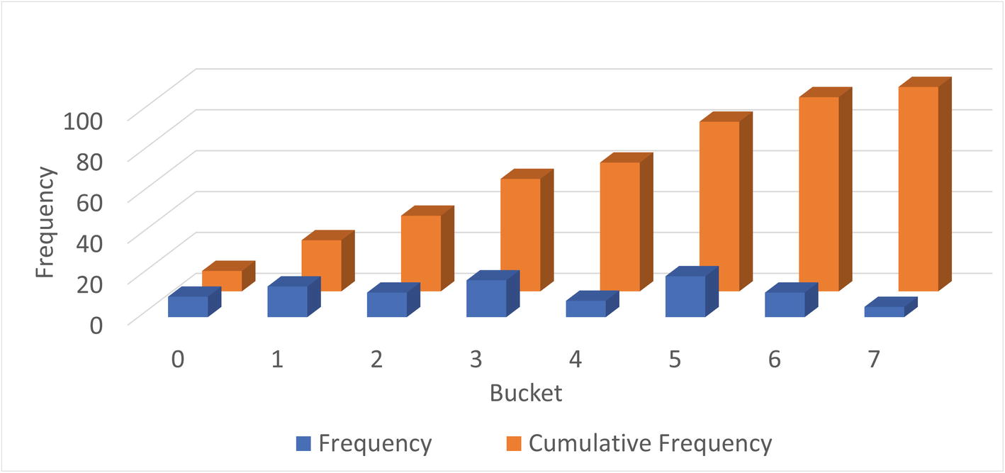
Values distributed into buckets and the cumulative frequency
In the figure, the dark columns in the front are the frequency of values in each bucket. The frequency is the percentage of the rows having that value. In the background (the brighter-colored columns) is the cumulative frequency which has the same value as the count column for bucket 0 and then increases gradually until it reaches 100 for bucket 7. What are cumulative frequencies? That is the second concept of histograms that you should understand.
Cumulative Frequencies
The cumulative frequency of a bucket is the percentage of rows that is in the current bucket and the previous buckets. If you are looking at bucket number 3 and the cumulative frequency is 50%, then 50% of the rows fit into buckets 0, 1, 2, and 3. This makes it very easy for the optimizer to determine the selectivity of a column with a histogram.
There are two scenarios to consider when the selectivity is calculated: an equality condition and a range condition. For an equality condition, the optimizer determines which bucket the value of the condition is in, then takes the cumulative frequency for that bucket, and subtracts the cumulative frequency of the previous bucket (for bucket 0, nothing is subtracted). If there is just one value in the bucket, that is all that is needed. Otherwise, the optimizer assumes each value in the bucket occurs at the same frequency, so the frequency for the bucket is divided with the number of values in the bucket.
Less Than: The cumulative frequency for the previous value is used.
Less Than or Equal: The cumulative frequency of the value in the condition is used.
Greater Than or Equal: The cumulative frequency of the previous value subtracted from 1.
Greater Than: The cumulative frequency of the value in the condition is subtracted from 1.
Histogram with one value per bucket
Bucket | Value | Cumulative Frequency |
|---|---|---|
0 | 0 | 0.1 |
1 | 1 | 0.25 |
2 | 2 | 0.37 |
3 | 3 | 0.55 |
4 | 4 | 0.63 |
5 | 5 | 0.83 |
6 | 6 | 0.95 |
7 | 7 | 1.0 |
In this example, the values are the same as the bucket numbers, but that is in general not the case. The cumulative frequency starts out with 0.1 (10%) and increases with the percentage of rows in each bucket until 100% is reached in the last bucket. This distribution is the same as that seen in Figure 16-1.
val = 4: The cumulative frequency of bucket 3 is subtracted from the cumulative frequency of bucket 4: estimate = 0.63 – 0.55 = 0.08. So 8% of the rows are estimated to be included.
val < 4: The cumulative frequency of bucket 3 is used, so 55% of the rows are estimated to be included.
val <= 4: The cumulative frequency of bucket 4 is used, so 63% of the rows are estimated to be included.
val >= 4: The cumulative frequency of bucket 3 is subtracted from 1, so 45% of the rows are estimated to be included.
val > 4: The cumulative frequency of bucket 4 is subtracted from 1, so 37% of the rows are estimated to be included.
Histogram with more than one value per bucket
Bucket | Values | Cumulative Frequency |
|---|---|---|
0 | 0-1 | 0.25 |
1 | 2-3 | 0.55 |
2 | 4-5 | 0.83 |
3 | 6-7 | 1.0 |
val = 4: The cumulative frequency of bucket 1 is subtracted from the cumulative frequency of bucket 2; then the result is divided with the number of values in bucket 2: estimate = (0.83 – 0.55)/2 = 0.14. So 14% of the rows are estimated to be included. This is higher than the more accurate estimate with one value per bucket as the frequencies for the values 4 and 5 are considered together.
val < 4: The cumulative frequency of bucket 1 is the only one that is required as buckets 0 and 1 include all values less than 4. Thus, it is estimated that 55% of the rows will be included (this is the same as for the previous example since in both cases the estimate only needs to consider complete buckets).
val <= 4: This is more complex as half the values in bucket 2 are included in the filtering and half are not. So the estimate will be the cumulative frequency for bucket 1 plus the frequency for bucket 2 divided with the number of values in the bucket: estimate = 0.55 + (0.83 – 0.55)/2 = 0.69 or 69%. This is higher and less accurate than the estimate using one value per bucket. The reason this estimate is less accurate is that it is assumed that values 4 and 5 have the same frequency.
val >= 4: This condition requires all values in buckets 2 and 3, so the estimate is to include 1 minus the cumulative frequency of bucket 1; that is 45% – the same as the estimate for the case with one value per bucket.
val > 4: This case is similar to val <= 4, just that the values to include are the opposite, so you can take the 0.69 and subtract from 1 which gives 0.31 or 31%. Again, since two buckets are involved, the estimate is not as accurate as for the single value per bucket.
As you have seen, there are two different scenarios when distributing the values into buckets: either there are at least as many buckets as values and each value can be assigned its own bucket or multiple values will have to share a bucket. These are two different types of histograms, and the specifics of those are discussed next.
Histogram Types
Singleton: For singleton histograms , there is exactly one value per bucket. These are the most accurate histograms as there is an estimate for every value that exists at the time the histogram is created.
Equi-height: When there are more values for the column than there are buckets, MySQL will distribute the values, so each bucket roughly has the same number of rows – that is, each bucket will be roughly the same height. Since all rows with the same value are distributed to the same bucket, the buckets will not be exactly the same height. For equi-height histograms, there are a different number of values represented for each bucket.
You have already encountered both histogram types when the cumulative frequencies were explored. The singleton histograms are the simplest and most accurate, but equi-height histograms are the most flexible as they can work with any data set.

A singleton histogram
The histogram has exactly one value per bucket. The frequencies range from 1.0% for Australia (AUS) to 24.9% for China (CHN). This is an example where a histogram can greatly help giving more accurate estimates of the filtering if there is no index on the CountryCode column. The original world.city table has 232 distinct CountryCode values, so a singleton histogram works well.
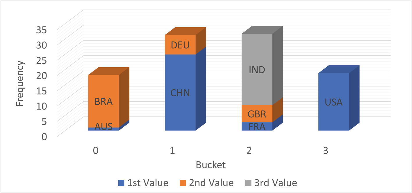
An equi-height histogram
For an equi-height histogram, MySQL aims at having the same frequency (height) of each bucket. However, since a column value will fully be in one bucket and values are distributed in sequence, it is in general not possible to get the exact same height. This is also the case in this example where buckets 0 and 3 have somewhat smaller frequencies than buckets 1 and 2.
The graph also shows a disadvantage of equi-height histograms. The high frequency of cities in Brazil (BRA), China (CHN), and India (IND) is somewhat masked by the low frequency of the countries they share buckets with. Thus, the accuracy of equi-height histograms is not as great as for singleton histograms. This is particularly the case when the frequencies of the values vary a lot. The reduced accuracy is in general a bigger issue for equality conditions than for range conditions, so equi-height histograms are best suited for columns mainly used for range conditions.
Before you can use the histogram statistics, you will need to create them, and once created you need to maintain the statistics. How to do that is the topic of the next section.
Adding and Maintaining Histograms
Histograms only exist as statistics unlike indexes that have a physical presence in the tablespaces. It is not too surprising then that histograms are created, updated, and dropped using the ANALYZE TABLE statement that is also used to update index statistics. There are two variants of the statement: to update and to drop the statistics. When creating and updating histograms, you also need to be aware of the sampling rate. This section goes through each of these topics.
Create and Update Histograms
You create or update a histogram by adding the UPDATE HISTOGRAM clause to the ANALYZE TABLE statement . If there are no statistics and a request to update is made, then the histogram is created; otherwise, the existing histogram is replaced. You will need to specify how many buckets that you want to divide the statistics into.
Optionally, you can add the NO_WRITE_TO_BINLOG or LOCAL keyword between ANALYZE and TABLE to avoid writing the statement to the binary log. This works the same way as when updating index statistics.
If you do not want to write the ANALYZE TABLE statement to the binary log, add the NO_WRITE_TO_BINLOG or LOCAL keyword, for example, ANALYZE LOCAL TABLE ....
Updating histograms for multiple columns
How many buckets should you choose? If you have fewer than 1024 unique values, it is recommended to have enough buckets to create a singleton histogram (i.e., at least as many buckets as unique values). If you choose more buckets than there are values, MySQL will just use the buckets needed to store the frequencies for each value. In this sense, the number of buckets should be taken as the maximum number of buckets to use.
If there are more than 1024 distinct values, you need enough buckets to get a good representation of the data. Between 25 and 100 buckets is often a good starting point. With 100 buckets, an equi-height histogram will on average have 1% of the rows in each bucket. The more uniform a distribution of the rows, the less buckets are needed, and the larger the difference in distribution, the more buckets are needed. Aim at having the most frequently occurring values in their own bucket. For example, for the subset of the world.city table used in the previous section, five buckets place China (CHN), India (IND), and the USA in their own buckets.
The histogram is created by sampling the values. How that is done depends on the amount of memory available.
Sampling
When MySQL creates a histogram, it needs to read the rows to determine the possible values and their frequencies. This is done in a similar but yet different way to sampling for index statistics. When the index statistics are calculated, the number of unique values is determined, which is a simple task as it just requires counting. Thus, all you need to specify is how many pages you want to sample.
For histograms, MySQL must determine not only the number of different values but also their frequency and how to distribute the values into buckets. For this reason, the sampled values are read into memory and then used to create the buckets and calculate the histogram statistics. This means that it is more natural to specify the amount of memory that can be used for the sampling rather than the number of pages. Based on the amount of memory available, MySQL will determine how many pages can be sampled.
In MySQL 8.0.18 and earlier, a full table scan is always required. In MySQL 8.0.19 and later, InnoDB can directly perform the sampling itself, so it can skip pages that will not be used in the sampling. This makes the sampling much more efficient for large tables. The sampled_pages_read and sampled_pages_skipped counters in information_schema.INNODB_METRICS provide statistics about the sampled and skipped pages for InnoDB.
The memory available during an ANALYZE TABLE .. UPDATE HISTOGRAM … statement is specified with the histogram_generation_max_mem_size option. The default is 20,000,000 bytes. The information_schema.COLUMN_STATISTICS view that is discussed in the “Inspecting Histogram Data” section includes information about the resulting sampling rate. If you do not get the expected accuracy of the filtering, you can check the sample rate, and if it is low, you can increase the value of histogram_generation_max_mem_size. The number of pages sampled scales linearly with the amount of memory available, whereas the number of buckets does not have any impact on the sampling rate.
Dropping a Histogram
Dropping histograms
The output of the ANALYZE TABLE statement is similar to creating statistics. You can also optionally add the NO_WRITE_TO_BINLOG or LOCAL keyword between ANALYZE and TABLE to avoid writing the statement to the binary log.
Once you have histograms, how do you inspect the statistics and the metadata of them? You can use the Information Schema for this as discussed next.
Inspecting Histogram Data
Knowing what information is available to the optimizer is important when the query plan is not what you expect. Like you have various views for the index statistics, the Information Schema also contains a view, so you can review the histogram statistics. The data is available through the information_schema.COLUMN_STATISTICS view. The next section includes examples of using this view to retrieve information about the histograms.
The COLUMN_STATISTICS view
Column Name | Data Type | Description |
|---|---|---|
SCHEMA_NAME | varchar(64) | The schema in which the table is located. |
TABLE_NAME | varchar(64) | The table in which the column for the histogram is located. |
COLUMN_NAME | varchar(64) | The column with the histogram. |
HISTOGRAM | json | The details of the histogram. |
The first three columns (SCHEMA_NAME, TABLE_NAME, COLUMN_NAME) form the primary key and allow you to query the histograms you are interested in. The HISTOGRAM column is the most interesting as it stores the metadata for the histogram as well as the histogram statistics.
The fields in the JSON document for the HISTOGRAM column
Field Name | JSON Type | Description |
|---|---|---|
buckets | Array | An array with one element per bucket. The information available for each bucket depends on the histogram type and is described later. |
collation-id | Integer | The id for the collation of the data. This is only relevant for string data types. The id is the same as the ID column in the INFORMATION_SCHEMA.COLLATIONS view. |
data-type | String | The data type of the data in the column the histogram has been created for. This is not a MySQL data type but rather a more generic type such as “string” for string types. Possible values are int, uint (unsigned integer), double, decimal, datetime, and string. |
histogram-type | String | The histogram type, either singleton or equi-height. |
last-updated | String | When the statistics were last updated. The format is YYYY-mm-dd HH:MM:SS.uuuuuu. |
null-values | Decimal | The fraction of the sampled values that is NULL. The value is between 0.0 and 1.0. |
number-of-buckets-specified | Integer | The number of buckets requested. For singleton histograms, this may be larger than the actual number of buckets. |
sampling-rate | Decimal | The fraction of pages in the table that were sampled. The value is between 0.0 and 1.0. When the value is 1.0, the whole table was read, and the statistics are exact. |
The view is not only useful to determine the histogram statistics, but you can also use it to check metadata, for example, to determine how long it has been since the statistics were last updated and use that to ensure the statistics are updated regularly.
The buckets field deserves some more attention as it is where the statistics are stored. It is an array with one element per bucket. The per bucket elements are themselves JSON arrays. For singleton histograms, there are two elements per bucket, whereas for equi-height histograms there are four elements.
Index 0: The column value for the bucket.
Index 1: The cumulative frequency.
Index 0: The lower bound of the column values included in the bucket.
Index 1: The upper bound of the column values included in the bucket.
Index 2: The cumulative frequency.
Index 3: The number of values included in the bucket.
If you go back and consider the examples of calculating the expected filtering effect of various conditions, you can see that the bucket information includes everything that is necessary, but also it does not include any extra information.
Since the histogram data is stored as a JSON document, it is worth having a look at a few example queries that retrieve various information.
Histogram Reporting Examples
The COLUMN_STATISTICS view is very useful for querying the histogram data. Since the metadata and statistics are stored in a JSON document, it is useful to consider some of the JSON manipulating functions that are available, so you can retrieve histogram reports. This section will show several examples of generating reports for the histograms you have in your system. All examples are also available from this book’s GitHub repository, for example, the query in Listing 16-3 is available in the file listing_16_3.sql.
List All Histograms
Listing all histograms
The query gives a high-level view of the histograms. The -> operator extracts a value from the JSON document, and the ->> operator additionally unquotes the extracted value which can be useful when extracting strings. From the example output, you can, for example, see that the histogram on the length column in the sakila.film table has 140 buckets but 256 buckets were requested. You can also see it is a singleton histogram, which is not surprising since not all requested buckets were used.
List All Information for a Single Histogram
Retrieving all data for a histogram
There are a couple of interesting things for this query. The JSON_PRETTY() function is used to make it easier to read the histogram information. Without the JSON_PRETTY() function, the whole document would be returned as a single line.
Notice also that the lower and upper bounds for each are returned as base64-encoded strings. This is to ensure that any value in string and binary columns can be handled by the histograms. Other data types have their values stored directly.
List Bucket Information for a Singleton Histogram
Listing the bucket information for a singleton histogram
Row_ID: This column has a FOR ORDINALITY clause which makes it a 1-based auto-increment counter, so it can be used for the bucket number by subtracting 1.
Bucket_Value: The column value used with the bucket. Notice that the value is returned after it has been decoded from its base64 encoding, so the same query works for strings and numeric values.
Cumulative_Frequency: The cumulative frequency for the bucket as a decimal number between 0.0 and 1.0.
The result of the JSON_TABLE() function can be used in the same way as a derived table. The cumulative frequency is in the SELECT part of the query converted to a percentage, and the LAG() window function2 is used to calculate the frequency (also as a percentage) for each bucket.
List Bucket Information for an Equi-height Histogram
The query to retrieve the bucket information for an equi-height histogram is very similar to the query just discussed for a singleton histogram. The only difference is that an equi-height histogram has two values (the start and end of the interval) defining the bucket and the number of values in the bucket.
Listing the bucket information for an equi-height histogram
Now you have some tools to inspect the histogram data, all that is left is to show an example of how histograms can change a query plan.
Query Example
The main goal of histograms is to help the optimizer to realize the optimal way to execute a query. It can be useful to see an example of how a histogram can influence the optimizer to change the query plan, so to round off this chapter, a query that changes the plan when a histogram is added to one of the columns in the WHERE clause will be discussed.
The film_id, title, and length columns come from the film table and the first_name and last_name columns from the actor table. The GROUP_CONCAT() function is used in case there is more than one actor in the movie that is named Elvis. (An alternative for this query is to use EXISTS(), but this way the full name of the actors with first name Elvis is included in the query result.)
There are no indexes on the length and first_name columns, so the optimizer cannot know how well the conditions on these columns filter. By default, it assumes that the condition on length returns around a third of the rows in the film table and that the condition on first_name returns 10% of the rows. (The next chapter includes where these default filter values come from.)
Figure 16-4 shows the query plan when no histograms exist. The query plan is shown as a Visual Explain diagram which will be discussed in Chapter 20.
You can create a Visual Explain diagram by executing the query in MySQL Workbench and clicking the Execution Plan button to the right of the query result.
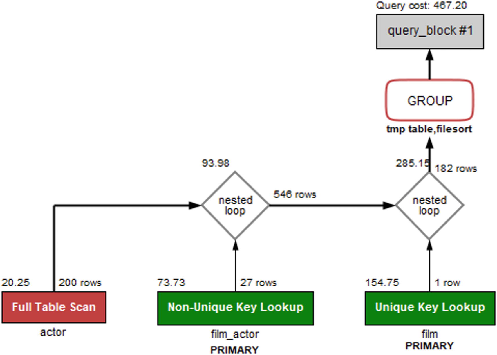
The query plan without a histogram
The important thing to notice in the query plan is that the optimizer has chosen to start with a full table scan on the actor table, then goes through the film_actor table, and finally joins on the film table. The total query cost (in the upper-right corner of the figure) is calculated as 467.20 (the query cost numbers in the diagram may differ from what you get as they depend on the index – and histogram – statistics).
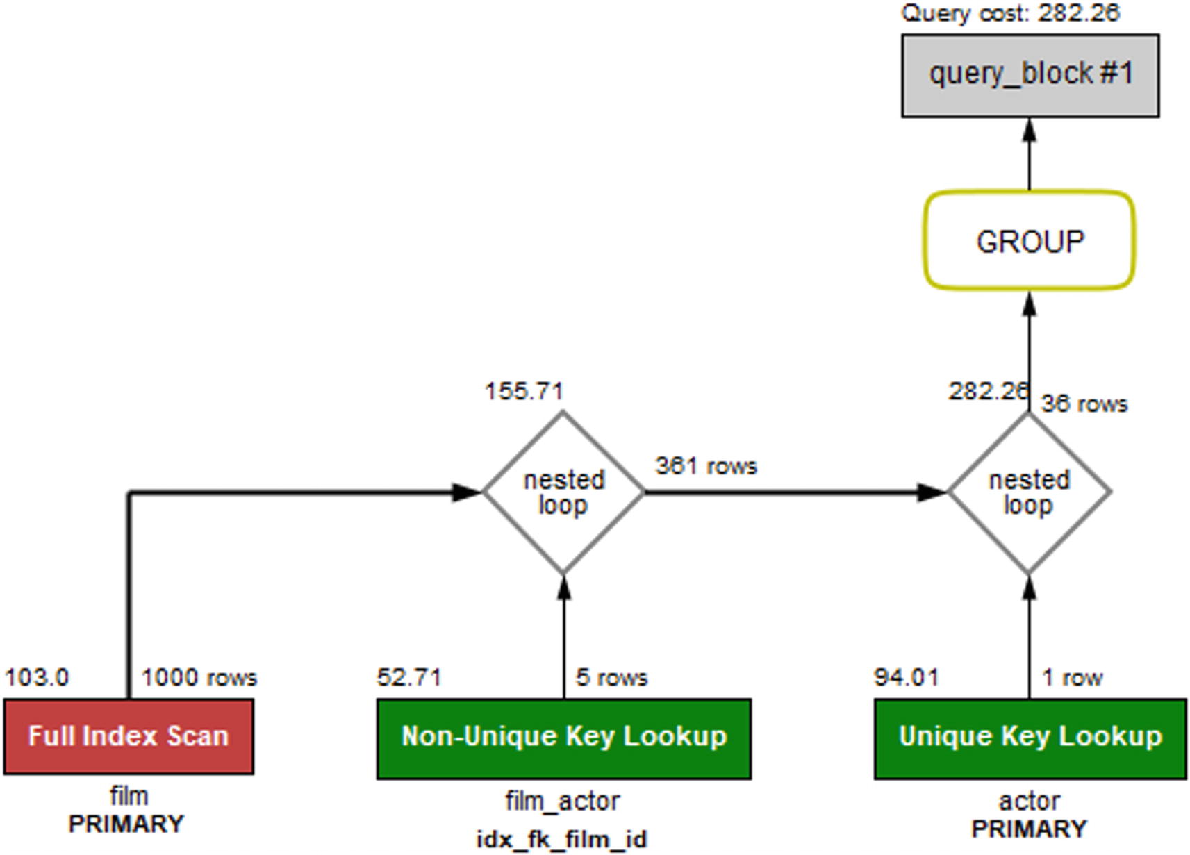
The query plan with a histogram on the length column
The histogram means that now the optimizer knows exactly how many rows will be returned if the film table is scanned first. This reduces the total cost of the query to 282.26 which is a good improvement. (Again, depending on your index statistics, you may see a different change. The important thing in the example is that the histogram changes the query plan and the estimated cost.)
In practice, there are so few rows in the tables used for this example that it hardly matters which order the query executes. However, in real-world examples, using a histogram can provide large gains, in some cases more than an order of magnitude.
What is also interesting with this example is that if you change the condition to look for movies shorter than 60 minutes, then the join order changes back to first scanning the actor table. The reason is that with that condition, enough films will be included based on the length that it is better to start finding candidate actors. In the same way, if you additionally add a histogram on the first_name of the actor table, the optimizer will realize the first name is a rather good filter for the actors in this database; particularly, there is only one actor named Elvis. It is left as an exercise for the reader to try to change the WHERE clause and the histograms and see how the query plan changes.
Summary
This chapter has shown how histograms can be used to improve the information the optimizer has available when it tries to determine the optimal query plan. Histograms divide the column values into buckets, either one value per bucket called a singleton histogram or multiple values per bucket called an equi-height histogram. For each bucket, it is determined how frequent the values are encountered, and the cumulative frequency is calculated for each bucket.
Histograms are mainly useful for columns that are not candidate to have indexes, but they are still used for filtering in queries featuring joins. In this case, the histogram can help the optimizer determine the optimal join order. An example was given at the end of the chapter showing how a histogram changes the join order for a query.
The metadata and statistics for a histogram can be inspected in the information_schema.COLUMN_STATISTICS view. The information includes all the data for each bucket that the optimizer uses as well as metadata such as when the histogram was last updated, the histogram type, and the number of buckets requested.
During the query example, it was mentioned that the optimizer has some defaults for the estimated filtering effect of various conditions. Thus far, in the discussion of indexes and histograms, the optimizer has mostly been ignored. It is time to change that: the next chapter is all about the query optimizer.