
Adding indexes to a table is a very powerful way to improve the query performance. An index allows MySQL to quickly find the data needed for a query. When the right indexes are added to your tables, query performance can potentially be improved by several orders of magnitude. The trick is to know which indexes to add. Why not just add indexes on all columns? Indexes have overhead as well, so you need to analyze your needs before adding random indexes.
This chapter starts out discussing what an index is, some index concepts, and what drawbacks adding an index can have. Then the various index types and features supported by MySQL are covered. The next part of the chapter starts out discussing how InnoDB uses indexes particularly related to index-organized tables. Finally, it is discussed how to choose which indexes you should add to your tables and when to add them.
What Is an Index?
In order to be able to use indexes to properly improve performance, it is important to understand what an index is. This section will not cover different index types – that will be discussed in the section “Index Types” later in the chapter – but rather the higher-level idea of an index.
The concept of an index is nothing new and existed well before computer databases became known. As a simple example, consider this book. At the end of the book, there is an index of some words and terms that have been selected as the most relevant search terms for the text in this book. The way that book index works is similar in concept to how database indexes work. It organizes the “terms” in the database, so your queries can find the relevant data more quickly than by reading all of the data and checking whether it matches the search criteria. The word terms is quoted here as it is not necessarily human-readable words that the index is made up of. It is also possible to index binary data such as spatial data.
In short, an index organizes your data in such a way that it is possible to narrow down the number of rows queries need to examine. The speedup from well-chosen indexes can be tremendous – several order of magnitudes. Again consider this book: if you want to read about B-tree indexes, you can either start from page 1 and keep reading the whole book or look up the term “B-tree index” in the book’s index and jump straight to the pages of relevance. When querying a MySQL database, the improvements are similar with the difference that queries can be much more complex than looking for information about something in a book, and thus the importance of indexes increases.
Clearly then, you just need to add all possible indexes, right? No. Other than the administrative complexity of adding the indexes, indexes themselves not only improve performance when used right; they also add overhead. So you need to pick your indexes with care.
Another thing is that even when an index can be used, it is not always more efficient than scanning the whole table. If you want to read significant parts of this book, looking up each term of interest in the index to find out where the topic is discussed and then going to read it will eventually become slower than just reading the whole book from cover to cover. In the same say, if your query anyway needs to access a large part of the data in the table, it will become faster to just read the whole table from one end to the other. Exactly what the threshold is where it becomes cheaper to scan the whole table depends on several factors. These factors include the disk type, the performance of sequential I/O compared to random I/O, whether the data fits in memory, and so on.
Before diving into the details of indexes, it is worth taking a quick look at some key indexing concepts.
Index Concepts
Given how big a topic indexes are, it is no surprise that there are several terms used to describe indexes. There are of course the names of the index types such as B-tree, full text, spatial, and so on, but there are also more general terms that are important to be aware of. The index types will be covered later in this chapter, so here the more general terms will be discussed.
Key Versus Index
You may have noticed that sometimes the word “index” is used and other times the word “key” is used. What is the difference? An index is a list of keys. However, in MySQL statements, the two terms are often interchangeable.
An example where it does matter is “primary key” – in that case, “key” must be used. On the other hand, when you add an index, you can write ALTER TABLE table_name ADD INDEX ... or ALTER TABLE table_name ADD KEY ... as you wish. The manual uses “index” in that case, so for consistency it is recommended to stick with index.
There are several terms to describe which kind of an index you are using. The first of these that will be discussed is a unique index.
Unique Index
A unique index is an index that only allows one row for each value in the index. Consider a table with data about people. You may include the social security number or a similar identifier for the person. No two persons should share social security numbers, so it makes sense to define a unique index on the column storing the social security number.
In this sense, “unique” more refers to a constraint than an indexing feature. However, the index part is critical for MySQL to be able to quickly determine whether a new value already exists.
Trigger checking for unique constraint violations
This handles any kind of duplicate values for the Name column. It uses the NULL safe equal operator (<=>) to determine whether the new value for Name already exists in the table. If it does, it quotes the value if it is not NULL and otherwise does not quote it, so it is possible to distinguish between the string “NULL” and the NULL value. Finally, a signal with SQL state 23000 and the MySQL error number 1062 is emitted. The error message, SQL state, and error number are the same as the normal duplicate key constraint error.
A special kind of unique index is the primary key.
Primary Key
The primary key for a table is an index which uniquely defines the row. NULL values are never allowed for a primary key. If you have multiple NOT NULL unique indexes on your table, either can serve the purpose of being the primary key. For reasons that will be explained shortly when discussing the clustered index, you should choose one or more columns with immutable values for the primary key. That is, aim at never changing the primary key for a given row.
The primary key is very special for InnoDB, while for other storage engines, it may more be a matter of convention. However, in all cases, it is best to always have some value that uniquely identifies a row as that, for example, allows replication to quickly determine which row to modify (more on this in Chapter 26), and the Group Replication feature explicitly requires all tables to have a primary key or a not NULL unique index. In MySQL 8.0.13 and later, you can enable the sql_require_primary_key option to require that all new tables must have a primary key. The restriction also applies if you change the structure of an existing table.
Enable the sql_require_primary_key option (disabled by default). Tables without a primary key can cause performance problems, sometimes in unexpected and subtle ways. This also ensures your tables are ready, if you want to use Group Replication in the future.
If there are primary keys, are there secondary keys as well?
Secondary Indexes
The term “secondary index” is used for an index that is not a primary key. It does not have any special meaning, so the name is just used to make it explicit that the index is not the primary key whether it is a unique or nonunique index.
As mentioned, the primary key has a special meaning for InnoDB as it is used for the clustered index.
Clustered Index
The clustered index is specific to InnoDB and is the term used for how InnoDB organizes the data. If you are familiar with Oracle DB, you may know of index-organized tables; that describes the same thing.
Everything in InnoDB is an index. The row data is in the leaf pages of a B-tree index (B-tree indexes will be described shortly). This index is called the clustered index. The name comes from the fact that index values are clustered together. The primary key is used for the clustered index. If you do not specify an explicit primary key, InnoDB will look for a unique index that does not allow NULL values. If that does not exist either, InnoDB will add a hidden 6-byte integer column using a global (for all InnoDB tables) auto-increment value to generate a unique value.
The choice of primary key also has performance implications. These will be discussed in the section “Index Strategies” later in the chapter. The clustered index can also be seen as a special case of a covering index. What is this? You are about to find out.
Covering Index
In this case, the query just needs the columns a and b, so it is not necessary to look up the rest of the row – the index is enough to retrieve all the required data. On the other hand, if the query also needs column c, the index is no longer covering. When you analyze a query using the EXPLAIN statement (this will be covered in Chapter 20) and a covering index is used for the table, the Extra column in the EXPLAIN output will include “Using index.”
A special case of a covering index is InnoDB’s clustered index (though EXPLAIN will not say “Using index” for it). The clustered index includes all the row data in the leaf node (even though in general only a subset of columns is actually indexed), so the index will always include all required data. Some databases support an include clause when creating indexes that can be used to simulate how the clustered index works.
Clever creation of indexes so they can be used as covering indexes for the most executed queries can greatly improve performance as it will be discussed in the “Index Strategies” section.
When you add indexes, there are some limitations you need to adhere to. These limitations are the next thing to cover.
Index Limitations
The maximum width of a B-tree index is 3072 bytes or 767 bytes depending on the InnoDB row format. The maximum size is based on 16 kiB InnoDB pages with lower limits for smaller page sizes.
Blob- and text-type columns can only be used in an index other than full text indexes when a prefix length is specified. Prefix indexes are discussed later in the chapter in the section “Index Features.”
Functional key parts count toward the limit of 1017 columns in a table.
There can be at most 64 secondary indexes on each table.
A multicolumn index can include at most 16 columns and functional key parts.
The limitation you are likely to encounter is the maximum index width for B-tree indexes. No index can be more than 3072 bytes when you use the DYNAMIC (the default) or COMPRESSED row format and no more than 767 bytes for the REDUNDANT and COMPACT row formats. The limit for tables using the DYNAMIC and COMPRESSED row formats is reduced to the half (1536 bytes) for 8 KiB pages and to a quarter (768 bytes) for 4 KiB pages. This is particularly a restriction for indexes on string and binary columns as not only are these values by nature often large, it is also the maximum possible amount of storage required that is used in the size calculation. That means that a varchar(10) using the utf8mb4 character set contributes 40 bytes to the limit even if you never store anything by single-byte characters in the column.
When you add a B-tree index to a text- or blob-type column, you must always provide a key length specifying how much of a prefix of the column you want to include in the index. This applies even for tinytext and tinyblob that only support 256 bytes of data. For char, varchar, binary, and varbinary columns, you only need to specify a prefix length if the maximum size of the values in bytes exceeds the maximum allowed index width for the table.
For text- and blob-type columns, instead of using a prefix index, it is often better to index using a full text index (more later), to add a generated column with the hash of the blob, or to optimize the access in some other way.
If you add functional indexes to a table, then each functional key part counts toward the limit for columns on a table. If you create an index with two functional parts, then this counts as two columns toward the table limit. For InnoDB there can be at most 1017 columns in a table.
The final two limitations are related to the number of indexes that can be included in a table and the number of columns and functional key parts you can have in a single index. You can have at most 64 secondary indexes on a table. In practice, if you are getting close to this limit, you can probably benefit from rethinking your indexing strategy. As it will be discussed in “What Are the Drawbacks of Indexes?” later in this chapter, there are overheads associated with indexes, so in all cases it is best to limit the number of indexes to those really benefitting queries. Similarly, the more parts you add to an index, the larger the index becomes. The InnoDB limit is that you can at most add 16 parts.
What do you do if you need to add an index to a table or remove a superfluous index? Indexes can be created together with the table or later, and it is also possible to drop indexes as discussed next.
SQL Syntax
When you first create your schema, you will in general have some ideas which indexes to add. Then as time passes, your monitoring may determine that some indexes are no longer needed but others should be added instead. These changes to indexes may be due to a misconception of the required indexes; the data may have changed, or the queries may have changed.
There are three distinct operations when it comes to changing the indexes on a table: creating indexes when the table itself is created, adding indexes to an existing table, or removing indexes from a table. The index definition is the same whether you add the index together with the table or as a following action. When dropping an index, you just need the index name.
This section will show the general syntax for adding and removing indexes. Throughout the rest of the chapter, there will be further examples based on the specific index types and features.
Creating Tables with Indexes
When you create a table, you can add the index definition to the CREATE TABLE statement. The indexes are defined right after the columns. You can optionally specify the name of the index; if you do not, the index will be named after the first column in the index.
Example of creating a table with indexes
This creates the table person with four indexes in the db1 schema (which must exist beforehand). The first is a primary key which is a B-tree index (more about that shortly) on the Id column. The second is also a B-tree index, but it is a so-called secondary index and indexes the Name column. The third index is a spatial index on the Location column. The fourth is a full text index on the Description column.
You can also create an index that includes more than a single column. This is useful if you need to put conditions on more than one column, put a condition on the first column and sort by the second, and so on. To create a multicolumn index, specify the column names as a comma-separated list:
INDEX (Name, Birthdate)
The order of the columns is very important as it will be explained in “Index Strategies.” In short, MySQL will only be able to use the index from the left, that is, the Birthdate part of the index can only be used if Name is also used. That means that the index (Name, Birthdate) is not the same index as (Birthdate, Name).
The indexes on a table will not in general remain static, so what do you do if you want to add an index to an existing table?
Adding Indexes
You can add indexes to an existing table, if you determine that is needed. To do this, you need to use the ALTER TABLE or CREATE INDEX statement. Since ALTER TABLE can be used for all modifications of the table, you may want to stick to that; however, the work made is the same with either statement.
Adding indexes using ALTER TABLE
The first and last ALTER TABLE statements use the ADD INDEX clause to tell MySQL that an index should be added to the table. The third statement adds two such clauses separated by a comma to add both indexes in one statement. In between, the index is dropped as it is bad practice to have duplicate indexes, and MySQL will also warn against it.
Does it make a difference if you use two statements to add two indexes or add both indexes with one statement? Yes, there can potentially be a big difference. When an index is added, it is necessary to perform a full table scan to read all the values needed for the index. A full table scan is an expensive operation for a large table, so in that sense, it is better to add both indexes in one statement. On the other hand, it is considerably faster to create the index as long as the index can be kept fully in the InnoDB buffer pool. Splitting the creation of the two indexes into two statements can reduce the pressure on the buffer pool and thus improve the index creation performance.
The last action is to remove indexes that are no longer needed.
Removing Indexes
The act of removing an index is similar to adding one. You can use the ALTER TABLE or DROP INDEX statement. When you use ALTER TABLE, you can combine dropping an index with other data definition manipulations of the table.
Find the index names for a table
Dropping an index using ATLER TABLE
This drops the index named name_2 – that is, the index on the (Name, Birthdate) columns.
The rest of this chapter will cover various details of what indexes are, and at the end of the chapter, the section “Index Strategies” discusses how to choose which data to index. First, it is important to understand why indexes have overhead.
What Are the Drawbacks of Indexes?
Very few things in life come for free – indexes are no exception. While indexes are great for improving query performance, they also need to be stored and kept up to date. Additionally, a less obvious overhead is when you execute a query, the more indexes you have, the more work the optimizer needs to do. This section will go through these three drawbacks of indexes.
Storage
One of the most obvious costs of adding an index is that the index needs to be stored, so it is readily available when it is needed. You do not want to first create the index each time it is needed as that would kill the performance benefit of the index.1 The storage overhead is twofold: the index is stored on disk to persist it, and it requires memory in the InnoDB buffer pool for queries to use it.
The disk storage means that you may need to add disks or block storage to your system. If you use a backup solution such as MySQL Enterprise Backup (MEB) that copies the raw tablespace files, your backups will also become larger and take longer to complete.
InnoDB always uses its buffer pool to read the data needed for a query. If the data does not already exist in the buffer pool, it is first read into it and then used for the query. So, when you use an index, both the index and the row data will in general be read into the buffer pool (one exception is when covering indexes are used). The more you need to fit into the buffer pool, the less room there is for other indexes and data – unless you make the buffer pool larger. It is of course more complex than that as avoiding a full table scan also prevents reading the whole table into the buffer pool which relieves the pressure on the buffer pool. The overall benefit versus overhead comes back to how much of the table you avoid examining by using the index and whether other queries anyway read the data the index otherwise avoids accessing.
All in all, you will need extra disk as you add indexes, and in general you will need a larger InnoDB buffer pool to keep the same buffer pool hit rate. Another overhead is that an index is only useful if it is kept up to date. That adds work when you update the data.
Updating the Index
Whenever you make changes to your data, the indexes will have to be updated. This ranges from adding or removing links to rows as data is inserted or deleted to modifying the index as values are updated. You may not think much of this, but it can be a significant overhead. In fact, during bulk data loads such as restoring a logical backup (a file that typically includes SQL statements for creating the data, e.g., created with the mysqlpump program), the overhead of keeping the indexes updated is often what limits the insert rate.
The overhead of keeping indexes up to date can be so high that it is generally recommended to remove the secondary indexes while doing a large import into an empty table and then recreate the indexes when the import has completed.
For InnoDB, the overhead also depends on whether the secondary indexes fit into the buffer pool or not. As long as the whole index is in the buffer pool, it is relatively cheap to keep the index up to date, and it is not very likely to become a severe bottleneck. If the index does not fit, InnoDB will have to keep shuffling the pages between the tablespace files and the buffer pool which is when the overhead becomes a major bottleneck causing severe performance problems.
There is one less obvious performance overhead as well. The more indexes, the more work for the optimizer to determine the optimal query plan.
The Optimizer
When the optimizer analyzes a query to determine what it believes is the optimal query execution plan, it needs to evaluate the indexes on each table to determine if the index should be used and possibly whether to do an index merge of two indexes. The goal is of course to have the query evaluate as quickly as possible. However, the time spent in the optimizer is in general non-negligible and in some cases can even become a bottleneck.
In this case, if there are no indexes on the table city, it is clear that a table scan is required. If there is one index, it is also necessary to evaluate the query cost using the index, and so forth. If you have a complex query involving many tables each with a dozen possible indexes, it will make for so many combinations that it will be reflected in the query execution time.
If the time spent in the optimizer becomes a problem, you can add optimizer and join order hints as discussed in Chapters 17 and 24 to help the optimizer, so it does not need to evaluate all possible query plans.
While these pages describing the overhead of adding indexes can make it sound like indexes are bad, do not avoid indexes. An index that has a great selectivity for queries that are executed frequently will be a great benefit. However, do not add indexes for the sake of adding indexes. It will be discussed at the end of the chapter in the section “Index Strategies” what some ideas to choosing indexes are, and there will also be examples in the rest of the book where indexes are discussed. Before getting that far, it is worth discussing the various index types supported by MySQL as well as other index features.
Index Types
B-tree indexes
Full text indexes
Spatial indexes (R-tree indexes)
Multi-valued indexes
Hash indexes
This section will go through these five index types and discuss what type of questions they can be used to speed up.
B-Tree Indexes
B-tree indexes are by far the most commonly used index type in MySQL. In fact, all InnoDB tables include at least one B-tree index as the data is organized in a B-tree index (the clustered index).
A B-tree index is an ordered index, so it is good at finding rows where you are looking for a column that is equal to some value, where a column is greater than or less than a given value, or where the column is between two values. This makes it a very useful index for many queries.
Another good feature of B-tree indexes is that they have predictable performance. As the name suggests, the index is organized as a tree starting with the root page and finishing with the leaf pages. InnoDB uses an extension of the B-tree index which is called B+-tree. The + means that the nodes at the same level are linked, so it is easy to scan the index without the need to go back up to the parent node when reaching the last record in a node.
In MySQL the terms B-tree and B+-tree are used interchangeably.
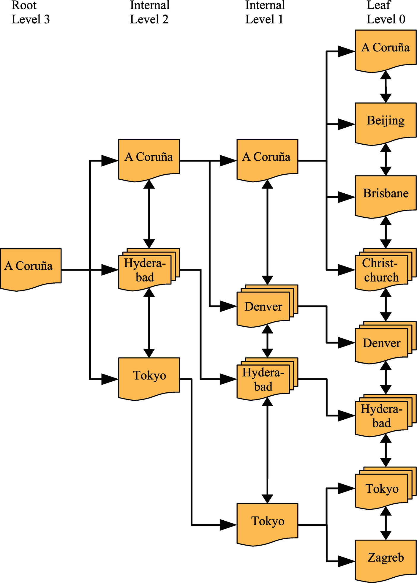
Example of a B+-tree index
In the figure, the document shapes represent an InnoDB page, and the shapes with multiple documents stacked on top of each other (e.g., the one in Level 0 labeled “Christchurch”) represent several pages. The arrows going from the left to the right go from the root page toward the leaf pages. The root page is where the index search starts, and the leaf pages are where the index records exist. Pages in between are typically called internal pages or branch pages. Pages may also be called nodes. The double arrows connecting the pages at the same level are what distinguishes a B-tree and a B+-tree index and allow InnoDB to quickly move to the previous or next sibling page without having to go through the parent.
For small indexes, there may only be a single page serving both as the root and leaf page. In the more general case, the index has a root page illustrated in the leftmost part of the figure. In the rightmost part of the figure are the leaf pages. For large indexes, there may also be more levels in between. The leaf nodes have Level 0, their parent pages Level 1, and so forth until the root page is reached.
In the figure, the value noted for a page, for example, “A Coruña,” denotes the first value covered by that part of the tree. So, if you are at Level 1 and are looking for the value “Adelaide,” you know it will be in the topmost page of the leaf pages as that page contains the values starting with “A Coruña” and finishing with the last value earlier than “Beijing” in the order the values are sorted. This is an example of where the collation discussed in the previous chapter comes into play.
A key feature is that irrespective of which of the branches you traverse, the number of levels will always be the same. For example, in the figure, that means no matter which value you look for, there will be four pages read, one for each of the four levels (if several rows have the same value and for range scans, more pages in the leaf level may be read). Thus, it is said that the tree is balanced. It is this feature that gives predictable performance, and the number of levels scales well – that is, the number of levels grows slowly with the number of index records. That is a property that is particularly important when the data needs to be accessed from relatively slow storage such as disks.
You may have heard of T-tree indexes as well. While B-tree indexes are optimized for disk access, T-tree indexes are similar to B-tree indexes except they are optimized for in-memory access. Therefore, the NDBCluster storage engine which stores all indexed data in memory uses T-tree indexes even when they at the SQL level are called B-tree indexes.
In the beginning of this section, it was stated that B-tree indexes are by far the most commonly used index type in MySQL. In fact, if you have any InnoDB tables, even if you never added any indexes yourself, you are using B-tree indexes. InnoDB stores the data index organized – using the clustered index – which really just means the rows are stored in a B+-tree index. B-tree indexes are also not just used in relational databases, for example, several file systems organize their metadata in a B-tree structure.
One property of B-tree indexes that is important to be aware of is that they can only be used for comparing the whole value of the indexed column(s) or a left prefix. This means that if you want to check if the month of an indexed date is May, the index cannot be used. This is the same if you want to check whether an indexed string contains a given phrase.
When you include multiple columns in an index, the same principle applies. Consider the index (Name, Birthdate): in this case, you can use the index to search for a given name or a combination of a name and a birthday. However, you cannot use the index to search for a person with a given birthdate without knowing the name.
There are several ways to handle this limitation. In some cases, you can use functional indexes, or you can extract information about the column into a generated column that you can index. In other cases, another index type can be used. As discussed next, a full text index can, for example, be used to search for columns with the phrase “query performance tuning” somewhere in the string.
Full Text Indexes
Full text indexes are specialized at answering questions such as “Which document contains this string?” That is, they are not optimized to find rows where a column exactly matches a string – for that, a B-tree index is a better choice.
A full text index works by tokenizing the text that is being indexed. Exactly how this is done depends on the parser used. InnoDB supports using a custom parser, but typically the built-in parser is used. The default parser assumes the text uses whitespace as the word separator. MySQL includes two alternative parsers: the ngram parser2 which supports Chinese, Japanese, and Korean and the MeCab parser which supports Japanese.
If you are planning to use full text indexes, it is recommended from a performance perspective to explicitly add the FTS_DOC_ID column and either set it as the primary key on the table or create a secondary unique index for it. The downside of creating the column yourself is that you must manage the values yourself.
Another specialized index type is for spatial data. Where full text indexes are for text documents (or strings), spatial indexes are for spatial data types.
Spatial Indexes (R-Tree)
Historically, spatial features have not been used much in MySQL. However, with support for spatial indexes in InnoDB in version 5.7 and additional improvements such as support for specifying a Spatial Reference System Identifier (SRID) for spatial data in MySQL 8, chances are that you may need spatial indexes at some point.
A typical use case for spatial indexes is a table with points of interest with the location of each point stored together with the rest of the information. The user may, for example, ask to get all electrical vehicle charging stations within 50 kilometers of their current location. To answer such a question as efficiently as possible, you will need a spatial index.
MySQL implements spatial indexes as R-trees. The R stands for rectangle and hints at the usage of the index. An R-tree index organizes the data such that points that are close in space are stored close to each other in the index. This is what makes it effective to determine whether a spatial value fulfills some boundary condition (e.g., a rectangle).
Using a spatial index
In the example, a table with city locations has a spatial index on the Location column. The Spatial Reference System Identifier (SRID) is set to 4326 to represent Earth. For this example, a single row is inserted, and a boundary is defined (if you are curious, then the boundary contains Australia). You can also specify the polygon directly in the MBRContains() function , but here it is done in two steps to make the parts of the query stand out clearer.
So spatial indexes help to answer if some geometrical shape is within some boundary. Similarly, a multi-valued index can help answer whether a given value is in a list of values.
Multi-valued Indexes
If you want to search all of the cities in your city collection and return those cities that have a suburb called “Surry Hills,” then you need a multi-valued index. MySQL 8.0.17 has added support for multi-valued indexes.
Preparing the mvalue_index table for multi-valued indexes
The UPDATE statement uses the JSON_ARRAYAGG() function to create a JSON array with three JSON objects, the district, name, and population, for each country. Finally, a SELECT statement is executed to return the names of the Australian cities.
The index extracts the name object from all elements of the cities array at the root of the doc document. The resulting data is casted to an array of char(35) values. The data type was chosen as the city table where the city names originate from is char(35). In the CAST() function, you use char for both the char and varchar data types.
Queries taking advantage of a multi-valued index
The two queries using MEMBER OF and JSON_CONTAINS() both look for countries that have a city named Sydney. The last query using JSON_OVERLAPS() looks for countries that have a city named Sydney or New York or both.
There is one index type left in MySQL: hash indexes.
Hash Indexes
If you want to search for rows where a column is exactly equal to some value, you can use a B-tree index as discussed earlier in the chapter. There is an alternative though: create a hash for each of the column values and use the hash to search for the matching rows. Why would you want to do that? The answer is that it is a very fast way to look up rows.
Hash indexes are not used much in MySQL. A notable exception is the NDBCluster storage engine that uses hash indexes to ensure uniqueness for the primary key and unique indexes and also uses them to provide fast lookups using those indexes. In terms of InnoDB, there is no direct support for hash indexes; however, InnoDB has a feature called adaptive hash indexes which is worth considering a little more.
The adaptive hash index feature works automatically within InnoDB. If InnoDB detects that you are using a secondary index frequently and adaptive hash indexes are enabled, it will build a hash index on the fly of the most frequently used values. The hash index is exclusively stored in the buffer pool and thus is not persisted, when you restart MySQL. If InnoDB detects that the memory can be used better for loading more pages into the buffer pool, it will discard part of the hash index. This is what is meant when it is said that it is an adaptive index: InnoDB will try to adapt it to be optimal for your queries. You can enable or disable the feature using the innodb_adaptive_hash_index option.
In theory, the adaptive hash index is a win-win situation. You get the advantages of having a hash index without the need to consider which columns you need to add it for, and the memory usage is all automatically handled. However, there is an overhead of having it enabled, and not all workloads benefit from it. In fact, for some workloads, the overhead can become so large that there are severe performance issues.
The metrics for the adaptive hash index in INNODB_METRICS
The number of successful searches using the adaptive hash index (adaptive_hash_searches) and the number of searches completed using the B-tree index (adaptive_hash_searches_btree) are enabled by default. You can use those to determine how often InnoDB resolves queries using the hash index compared to the underlying B-tree index. The other metrics are less often needed and thus disabled by default. That said, if you want to explore the usefulness of the adaptive hash index in more detail, you can safely enable the six metrics.
Using the InnoDB monitor to monitor the adaptive hash index
The first point to check is the semaphores section. If the adaptive hash index is a major source of contention, there will be semaphores around the btr0sea.ic file (where the adaptive hash index is implemented in the source code). If you once in a while – but rarely – see semaphores, it is not necessarily a problem, but if you see frequent and long semaphores, you are likely better off disabling the adaptive hash index.
The other part of interest is the section for the insert buffer and adaptive hash index. This includes the amount of memory used for the hash indexes and the rate queries are answered using hash and non-hash searches. Be aware that these rates are for the period listed near the top of the monitor output – in the example, for the last 16 seconds prior to 2019-05-05 17:22:14.
That concludes the discussion of the supported index types. There is still more to indexes as there are several features that are worth familiarizing yourself with.
Index Features
It is one thing to know which types of indexes exist, but another thing is to be able to get the full advantage of them. For that to happen, you need to know more about the index-related features that are available in MySQL. These range from sorting the values in the index in reverse order to functional indexes and auto-generated indexes. This section will go through these features, so you can use them in your daily work.
Functional Indexes
If you add an index on the Birthdate column, this cannot be used to answer that query as the dates are stored according to their full value and you are not matching against the leftmost part of the column. (On the other hand, searching for all born in 1970 can use a B-tree index on the Birthdate column.)
The advantage of using the functional index is that is it more explicit what you want to index, and you do not have the extra BirthMonth column. Otherwise, the two ways of adding functional indexes work the same way.
Prefix Indexes
It is not uncommon for the index part of a table to become larger than the table data itself. This can particularly be the case if you index large string values. There are also limitations on the maximum length of the indexed data for B-tree indexes – 3072 bytes for InnoDB tables using the DYNAMIC or COMPRESSED row format and smaller for other tables. This effectively means you cannot index a text column, not to mention a longtext column. One way to mitigate large string indexes is to only index the first part of the value. That is called a prefix index.
The frequency of city names based on the first ten characters
This shows that with this index prefix, you will at most read six cities to find a match. While that is more than a complete match, it is still much better than scanning all the table. In this comparison, you of course also need to verify whether the number of prefix matches is due to prefix collisions, or the city names are the same. For example, for “Cambridge,” there are three cities with that name, so whether you index the first ten characters or the whole name makes no difference. You can do this kind of analysis for different prefix lengths to get an idea for the threshold where increasing the size of the index gives a diminutive return. In many cases, you do not need all that many characters for the index to work well.
What do you do if you believe you can delete an index or you want to roll out an index but not let it take effect immediately? The answer is invisible indexes.
Invisible Indexes
MySQL 8 has introduced a new feature called invisible indexes . It allows you to have an index that is maintained and ready for use, but the optimizer will ignore the index until you decide to make it visible. This allows you to roll out a new index in a replication topology or to disable an index you believe is not required or similar. You can quickly enable or disable the index as it only requires an update of the metadata for the table, so the change is “instant.”
If you, for example, believe an index is not needed, making it invisible first allows you to monitor how the database works without it before telling MySQL to drop the index. Should it turn out that some queries – for example, monthly reporting queries that just had not been executed in the period you monitored – do need the index, you can quickly reenable it.
You can override the invisibility of an index by enabling the optimizer switch use_invisible_indexes (defaults to off). This can be useful if you experience problems because an index has been made invisible and you cannot reenable it immediately or if you want to test with a new index before making it generally available. An example of temporarily enabling invisible indexes for a connection is
SET SESSION optimizer_switch = 'use_invisible_indexes=on';
Even with the use_invisible_indexes optimizer switch enabled, you are not allowed to refer to the index in an index hint.
Another new feature in MySQL 8 is descending indexes.
Descending Indexes
In MySQL 5.7 and older, when you added a B-tree index, it was always sorted in ascending order. This is great for finding exact matches, retrieving rows in ascending order of the index, and so on. However, while ascending indexes can speed up queries looking for rows in descending order, they are not as effective. MySQL 8 added descending indexes to help with those use cases.
If there are multiple columns in the index, the columns do not all need to be included in ascending or descending order. You can mix ascending and descending columns as it works best in your queries.
Partitioning and Indexes
If you create a partitioned table, the partitioning column must be part of the primary key and all unique keys. The reason for this is that MySQL does not have a concept of global indexes, so it must be ensured that uniqueness checks only need to consider a single partition.
With respect to performance tuning, then partitions can be used to effectively use two indexes to resolve a query without using index merging. When the column that is used for partitioning is used in a condition in a query, MySQL will prune the partitions, so only the partitions that can be matched by the condition are searched. Then an index can be used to resolve the rest of the query.
Combining partition pruning and filtering using an index
The t_part table is partitioned by range using the Unix timestamp of the Created column. The EXPLAIN output (EXPLAIN is covered in detail in Chapter 20) shows that only the p201903 partition will be included in the query and that the val index will be used as the index. The exact output of EXPLAIN may differ given the example uses random data.
Thus far, everything that has been discussed about indexes has been for explicitly created indexes. For certain queries, MySQL will also be able to auto-generate indexes. That is the last index feature to discuss.
Auto-generated Indexes
For queries that include subqueries joined to other tables or subqueries, the join can be expensive as subqueries cannot include explicit indexes. To avoid doing full table scans on these temporary tables generated by subqueries, MySQL can add an automatically generated index on the join condition.
MySQL chooses to do a full table scan on the film table and add an auto-generated index on the subquery. When MySQL adds an auto-generated index, the EXPLAIN output will include <auto_key0> (or 0 replaced with a different value) as the possible key and used key.
Auto-generated indexes can drastically improve the performance of queries that include subqueries that the optimizer cannot rewrite as normal joins. The best of it all is that it happens automatically.
That concludes the discussion of index features. Before discussing how you should use indexes, it is also necessary to understand how InnoDB uses indexes.
InnoDB and Indexes
The way InnoDB has organized its tables since its first versions in the mid-1990s has been to use a clustered index to organize the data. This fact has led to the common saying that everything in InnoDB is an index. The organization of the data is literally an index. By default, InnoDB uses the primary key for the clustered index. If there is no primary key, it will look for a unique index not allowing NULL values. As a last resort, a hidden column will be added to the table using a sort of auto-increment counter.
With index-organized tables, it is true that everything in InnoDB is an index. The clustered index is itself organized as a B+-tree index with the actual row data in the leaf pages. This has some consequences when it comes to query performance and indexes. The next sections will look at how InnoDB uses the primary key and what it means for secondary keys, provide some recommendations, and look at the optimal use cases for index-organized tables.
The Clustered Index
Since the data is organized according to the clustered index (the primary key or substitutes thereof), the choice of primary key is very important. If you insert a new row with a primary key value between existing values, InnoDB will have to reorganize the data to make room for the new row. In the worst case, InnoDB will have to split existing pages into two as the pages are fixed size. Page splits can cause the leaf pages to be out of order on the underlying storage causing more random I/O which in turn leads to worse query performance. Page splits will be discussed as part of the DDL and bulk data loading in Chapter 25.
Secondary Indexes
The leaf pages of a secondary index store the reference to the row itself. Since the row is stored in a B+-tree index according to the clustered index, all secondary indexes must include the value of the clustered index. If you have chosen a column where the values require many bytes, for example, a column with long and potentially multi-byte strings, this greatly adds to the size of the secondary indexes.
It also means that effectively when you perform a lookup using a secondary index, then two index lookups are made: first is the expected secondary key lookup, and then from the leaf page, the primary key value is fetched and used for a primary key lookup to get the actual data.
For nonunique secondary indexes, if you have an explicit primary key or a NOT NULL unique index, it is the columns used for the primary key that are added to the index. MySQL knows about these extra columns even though they have not been explicitly made part of the index, and MySQL will use them if it will improve the query plan.
Recommendations
Because of the way InnoDB uses the primary key and how it is added to the secondary indexes, it is best to use a monotonical incrementing primary key that uses as few bytes as possible. An auto-incrementing integer fulfills these properties and thus makes a good primary key.
The hidden column used for the clustered index if the table does not have any suitable indexes uses an auto-increment–like counter to generate new values. However, as that counter is global for all InnoDB tables in the MySQL instance with a hidden primary key, it can become a contention point. The hidden key also cannot be used in replication to locate the rows that are affected by an event, and Group Replication requires a primary key or NOT NULL unique index for its conflict detection. The recommendation is therefore always to explicitly choose a primary key for all tables.
An UUID on the other hand is not monotonical incrementing and is not a good choice. An option in MySQL 8 is to use the UUID_TO_BIN() function with a second argument set to 1 which will make MySQL swap the first and third groups of hexadecimal digits. The third group is the high field of the timestamp part of the UUID, so bringing that up to the beginning of the UUID helps ensure the IDs keep increasing and storing them as binary data requires less than half the amount of storage compared to hexadecimal values.
Optimal Use Cases
Index-organized tables are particularly useful for queries that use that index. As the name “clustered index” suggests, rows that have similar values for the clustered index are stored near each other. Since InnoDB always reads entire pages into memory, it also means that two rows with similar values for the primary key are likely read in together. If you need both in your query or in queries executed shortly after each other, the second row is already available in the buffer pool.
You should now have a good background knowledge of indexes in MySQL and how InnoDB uses indexes including its organization of data. It is time to put it all together and discuss index strategies.
Index Strategies
The big question when it comes to indexes is what to index and secondly what kind of index and which index features to use. It is not possible to create ultimate step-by-step instructions to ensure the optimal indexes; for that, experience and good understanding of the schema, data, and queries are required. It is however possible to give some general guidelines as it will be discussed in this section.
The first thing to consider is when you should add the indexes; whether you should do it at the time you originally create the table or later. Then there is the choice of primary key and the considerations how to choose it. Finally, there are the secondary indexes including how many columns to add to the index and whether the index can be used as a covering index.
When Should You Add or Remove Indexes?
Index maintenance is a never-ending task. It starts when you first create the table and continues throughout the lifetime of the table. Do not take index work lightly – as mentioned, the difference between great and poor indexing can be several orders of magnitude. You cannot buy yourself out of a situation with poor indexes by pouring more hardware resources at it. Indexes affect not only the raw query performance but also locking (as will be further discussed in Chapter 18), memory usage, and CPU usages.
When you create the table, you should particularly spend time on choosing a good primary key. The primary key will typically not change during the life of the table, and if you do decide to change the primary key, with index-organized tables it will necessarily require a full rebuild of the table. Secondary indexes can to a larger degree be tuned over time. In fact, if you plan on importing a large amount of data for the initial population of the table, it is best to wait to add the secondary indexes until after the data has been loaded. A possible exception is unique indexes as they are required for data validation.
schema_tables_with_full_table_scans: This view shows all tables where rows are read without using an index and ordered in descending order by that number. If a table has a large number of rows read without using an index, you can look for queries using this table and see if indexes can help. The view is based on the table_io_waits_summary_by_index_usage Performance Schema table which can also be used directly, for example, if you want to do a more advanced analysis, such as finding the percentage of rows read without using an index.
statements_with_full_table_scans: This view shows the normalized version of the statements that do not use an index at all or do not use a good index. The statements are ordered by the number of times they have been executed without using an index at all and then by the number of times they have not been using a good index – both in descending order. The view is based on the events_statements_summary_by_digest Performance Schema table.
Chapters 19 and 20 will cover the use of these views and the underlying Performance Schema tables in more detail.
When you identify that queries can benefit from additional indexes, then you need to evaluate whether the cost of having an extra benefit is worth the gain when executing the query.
schema_index_statistics: This view has statistics for how often an index is used to read, insert, update, and delete rows using a given index. Like the schema_tables_with_full_table_scan view, schema_index_statistics is based on the table_io_waits_summary_by_index_usage Performance Schema table.
schema_unused_indexes: This view will return the names of the indexes that have not been used since the data was last reset (no longer than since the last restart). This view is also based on the table_io_waits_summary_by_index_usage Performance Schema table.
schema_redundant_indexes: If you have two indexes covering the same columns, you double the amount of effort for InnoDB to keep the indexes up to date and add a burden on the optimizer, but do not gain anything. The schema_redundant_indexes view can as the name suggests be used to find redundant indexes. The view is based on the STATISTICS Information Schema table.
When you use the first two of these views, you must remember that the data comes from in-memory tables in the Performance Schema. If you have some queries that are only executed very occasionally, the statistics may not reflect what your overall index needs are. This is one of the cases where the invisible index feature can come in handy as it allows you to disable the index and at the same time keep the index until you are sure it is safe to drop it. If it turns out some rarely executed queries need the index, you can easily enable the index again.
As mentioned, the first consideration is what to choose as the primary key. Which columns should you include? That is the next thing to discuss.
Choice of the Primary Key
When you work with index-organized tables, the choice of the primary index is very important. The primary key can impact the ratio between random and sequential I/O, the size of secondary indexes, and how many pages need to be read into the buffer pool. The primary key for InnoDB tables is always a B+-tree index.
An optimal primary key with respect to the clustered index is as small (in bytes) as possible, keeps increasing monotonically, and groups the rows you query frequently and within short time of each other. In practice, it may not be possible to fulfill all of this in which case you need to make the best possible compromise. For many workloads, an auto-incrementing unsigned integer, either int or bigint depending on the number of rows that are expected for the table, is a good choice; however, there may be special considerations such as requirements for uniqueness across multiple MySQL instances. The most important feature of the primary key is that it should be as sequential as possible and immutable. If you change the value of the primary key for a row, it requires moving the whole row to the new position in the clustered index.
An unsigned integer that auto-increments is often a good choice as a primary key. It keeps incrementing monotonically, it does not require much storage, and it groups recent rows together in the clustered index.
You may think that the hidden primary key may be as good a choice for the clustered index as any other column. After all, it is an auto-incrementing integer. However, there are two major drawbacks of the hidden key: it only identifies the row for that local MySQL instance, and the counter is global to all InnoDB tables (in the instance) without a user-defined primary key. That the hidden key is only useful locally means that in replication, the hidden value cannot be used to identify which row to update on replicas. That the counter is global means that it can become a point of contention and cause performance degradation when inserting data.
The bottom line is that you should always explicitly define what you want as your primary key. For secondary indexes, there are more choices as it will be seen next.
Adding Secondary Indexes
Secondary indexes are all those indexes that are not the primary key. They can be either unique or not unique, and you can choose between all the supported index types and features. How do you choose which indexes to add? This section will make it easier for you to make that decision.
Be careful not to add too many indexes to a table up front. Indexes have overhead, so when you add indexes that end up not being used, queries and the system overall will perform worse. This does not mean you should not add any secondary indexes when you create the table. It’s just that you need to put some thought into it.
Reduce the rows examined: This is used when you have a WHERE clause or join condition to find the required rows without scanning the whole table.
Sort data: B-tree indexes can be used to read the rows in the order the query needs allowing MySQL to bypass the ordering step.
Validate data: This is what the uniqueness in unique indexes is used for.
Avoid reading the row: Covering indexes can return all the required data without reading the whole row.
Find MIN() and MAX() values: For GROUP BY queries, the minimum and maximum values for an indexed column can be found by just checking the first and last records in the index.
The primary key can obviously also be used for all these purposes. From a query perspective, there is no difference between a primary key and a secondary key.
When you need to decide whether to add an index, you need to ask yourself which of the purposes the index is needed for and whether it will be able to fulfill them. Once you have confirmed that it is the case, you can look at which order columns should be added in for multicolumn indexes and whether additional columns should be added. The next two subsections will discuss this in more detail.
Multicolumn Index
You can add up to 16 columns or functional parts to an index as long as you do not exceed the maximum width of the index. This applies both for the primary key and for secondary indexes. InnoDB has a limit of 3072 bytes per index. If you include strings using variable width character sets, then it is the maximum possible width that counts toward the index width.
You can use an index on the CountryCode column to look for cities with the country code set to AUS, and you can use an index on the Population column to look for cities with a population greater than 1 million. Even better, you can combine it into one index that includes both columns.
In this example, the index can even be used to order the result using the population.
If you need to add several columns that all are used for equality conditions, then there are two things to consider: which columns are most often used and how well does the column filter the data. When there are multiple columns in an index, MySQL will only use a left prefix of the index. If you, for example, have an index (col_a, col_b, col_c), you can only use the index to filter on col_b, if you also filter on col_a (and that must be an equality condition). So you need to choose the order carefully. In some cases, it can be necessary to add more than one index for the same columns where the column order differs between the indexes.
If you cannot decide in which order to include the columns based on the usage, then add them with the most selective column first. The next chapter will discuss selectivity of indexes, but in short, the more distinct values a column has, the more selective it is. By adding the most selective columns first, you will more quickly narrow down the number of rows that the part of the index contains.
You may also want to include columns that are not used for filtering. Why would you want to do that? The answer is that it can help form a covering index.
Covering Indexes
A covering index is an index on a table where the index for a given query includes all columns needed from that table. This means that when InnoDB reaches the leaf page of the index, it has all the information it needs, and it does not need to read the whole row. Depending on your table, this can potentially give a good improvement in query performance, particularly if you can use it to exclude large parts of the row such as large text or blob columns.
You can also use a covering index to simulate a secondary clustered index. Remember that the clustered index is just a B+-tree index with the whole row included in the leaf pages. A covering index has a complete subset of the rows in the leaf pages and thus emulates a clustered index for that subset of columns. Like for a clustered index, any B-tree index groups similar values together, and thus it can be used to reduce the number of pages read into the buffer pool, and it helps doing sequential I/O when you perform an index scan.
There are a couple of limitations for a covering index compared to a clustered index though. A covering index only emulates a clustered index for reads. If you need to write data, the changes always must access the clustered index. Another thing is that due to InnoDB’s multi-version concurrency control (MVCC), even when you use a covering index, it is necessary to check the clustered index to verify whether another version of the row exists.
When you add an index, it is worth considering which columns will be needed for the queries the index is intended for. It may be worth adding any extra columns used in the select part even if the index will not be used for filtering or sorting on those columns. You need to balance the benefit of the covering index with the added size of the index. Thus, this strategy is mostly useful if you just miss one or two small columns. The more queries the covering index benefits, the more extra data you can accept adding to the index.
Summary
This chapter has been a journey through the world of indexes. A good indexing strategy can mean the difference of a database coming to a grinding halt and a well-oiled machine. Indexes can help reduce the number of rows examined in queries, and additionally covering indexes can avoid reading the whole row. On the other hand, there are overheads associated with indexes both in terms of storage and ongoing maintenance. It is thus necessary to balance out the need for indexes and the cost of having them.
MySQL supports several different index types. The most important is B-tree indexes which are also what InnoDB uses to organize the rows in its index-organized tables using a clustered index. Other index types include full text indexes, spatial (R-tree) indexes, multi-valued indexes, and hash indexes. The latter type is special in InnoDB as it is only supported using the adaptive hash index feature which decides which hash indexes to add automatically.
There is a range of index features that have been discussed. Functional indexes can be used to index the result of using a column in an expression. Prefix indexes can be used to reduce the size of indexes for text and binary data types. Invisible indexes can be used during a rollout of new indexes or when soft deleting existing indexes. Descending indexes improve the effectiveness of traversing the indexed values in descending order. Indexes also play a role in connection with partitioning, and you can use partitioning to effectively implement support for using two indexes for a single table in a query. Finally, MySQL is able to auto-generate indexes in connection with subqueries.
The final part of the chapter started out with the specifics of InnoDB and the considerations of using index-organized tables. These are optimal for primary key–related queries but work less well for data inserted in random primary key order and querying data by secondary indexes.
The last section discussed indexing strategies. Choose your primary key carefully when you first create the table. Secondary indexes can to a larger extent be added and removed over time based on observations of metrics. You can use multicolumn indexes to use the index to filter on multiple columns and/or for sorting. Finally, covering indexes can be used to emulate secondary clustered indexes.
This concludes the discussion of what indexes are and when to use them. There is a little more to indexes as will be seen in the next chapter when index statistics are discussed.