
In the previous chapter, you learned how to find queries that are candidates for optimization. It is now time to take the next step – analyzing the queries to determine why they do not perform as expected. The main tool during the analysis is the EXPLAIN statement which shows the query plan the optimizer will use. Related is the optimizer trace that can be used to investigate why the optimizer ended up with the query plan. Another possibility is to use the statement and stage information in the Performance Schema to see where a stored procedure or a query spends the most time. These three topics will be discussed in this chapter.
EXPLAIN Usage: The basic usage of the EXPLAIN statement.
EXPLAIN Formats: The details specific to each of the formats that the query plan can be viewed in. This includes both formats explicitly chosen with the EXPLAIN statement and Visual Explain used by MySQL Workbench.
EXPLAIN Output: A discussion of the information available in the query plans.
EXPLAIN Examples: Some examples of using the EXPLAIN statement with a discussion of the data returned.
EXPLAIN Usage
The EXPLAIN statement returns an overview of the query plan the MySQL optimizer will use for a given query. It is at the same time very simple and one of the more complex tools in query tuning. It is simple, because you just need to add the EXPLAIN command before the query you want to investigate, and complex because understanding the information requires some understanding of how MySQL and its optimizer work. You can use EXPLAIN both with a query you explicitly specify and with a query currently being executed by another connection. This section goes through the basic usage of the EXPLAIN statement.
Usage for Explicit Queries
You generate the query plan for a query by adding EXPLAIN in front of the query, optionally adding the FORMAT option to specify whether you want the result returned in a traditional table format, using the JSON format, or in a tree-style format. There is support for SELECT, DELETE, INSERT, REPLACE, and UPDATE statements. The query is not executed (but see the next subsection about EXPLAIN ANALYZE for an exception), so it is safe to obtain the query plan.
If you need to analyze composite queries such as stored procedures and stored functions, you will need first to split the execution out into individual queries and then use EXPLAIN for each of the queries that should be analyzed. One method to determine the individual queries in a stored program is to use the Performance Schema. An example of achieving this will be shown later in this chapter.
Which format that is the preferred depends on your needs. The traditional format is easier to use when you need an overview of the query plan, the indexes used, and other basic information about the query plan. The JSON format provides more details and is easier for an application to use. For example, Visual Explain in MySQL Workbench uses the JSON-formatted output.
The tree format is the newest format and supported in MySQL 8.0.16 and later. It requires the query to be executed using the Volcano iterator executor which at the time of writing is not supported for all queries. A special use of the tree format is for the EXPLAIN ANALYZE statement.
EXPLAIN ANALYZE
The EXPLAIN ANALYZE statement 1 is new as of MySQL 8.0.18 and is an extension of the standard EXPLAIN statement using the tree format. The key difference is that EXPLAIN ANALYZE actually executes the query and, while executing it, statistics for the execution are collected. While the statement is executed, the output from the query is suppressed so only the query plan and statistics are returned. Like for the tree output format, it is required that the Volcano iterator executor is used.
At the time of writing, the requirement on the Volcano iterator executor limits the queries you can use EXPLAIN ANALYZE with to a subset of SELECT statements. It is expected that the range of supported queries will increase over time.
The output of EXPLAIN ANALYZE will be discussed together with the tree format output later in this chapter.
By nature, EXPLAIN ANALYZE only works with an explicit query as it is required to monitor the query from start to finish. The plain EXPLAIN statement on the other hand can also be used for ongoing queries.
Usage for Connections
Imagine you are investigating an issue with poor performance and you notice there is a query that has been running for several hours. You know this is not supposed to happen, so you want to analyze why the query is so slow. One option is to copy the query and execute EXPLAIN for it. However, this may not provide the information you need as the index statistics may have changed since the slow query started, and thus analyzing the query now does not show the actual query plan causing the slow performance.
This will take around 420 seconds (0.1 second per row in the world.city table).
You can optionally add which format you want in the same way as when you explicitly specify a query. The filtered column may show 100.00 if you are using a different client than MySQL Shell. Before discussing what the output means, it is worth familiarizing yourself with the output formats.
EXPLAIN Formats
You can choose between several formats when you need to examine the query plans. Which one you choose mostly depends on your preferences. That said, the JSON format does include more information than the traditional and tree formats. If you prefer a visual representation of the query plan, Visual Explain from MySQL Workbench is a great option.
The query finds the five largest cities across the ten smallest countries by area in Europe and orders them by the city population in descending order. The reason for choosing this query is that it shows how the various output formats represent subqueries, ordering, and limits. The information returned by the EXPLAIN statements will not be discussed in this section; that is deferred to the “EXPLAIN Examples” section.
The output of EXPLAIN statements depends on the settings of the optimizer switches, the index statistics, and the values in the mysql.engine_cost and mysql.server_cost tables, so you may not see the same as in the examples. The example outputs have been used with the default values and a freshly loaded world sample database with ANALYZE TABLE executed for the tables after the load has completed, and they have been created in MySQL Shell where warnings are fetched automatically by default (but the warnings are only included in the output when they are discussed). If you are not using MySQL Shell, you will have to execute SHOW WARNINGS to retrieve the warnings.
This convention is used throughout the chapter.
Traditional Format
When you execute the EXPLAIN command without the FORMAT argument or with the format set to TRADITIONAL , the output is returned as a table as if you had queried a normal table. This is useful when you want an overview of the query plan and it is a human database administrator or developer who examines the output.
The table output can be quite wide particularly if there are many partitions, several possible indexes that can be used, or several pieces of extra information. You can request to get the output in a vertical format by using the --vertical option when you invoke the mysql command-line client, or you can use G to terminate the query.
Example of the traditional EXPLAIN output
Notice how the first table is called <derived 2>. This is for the subquery on the country table, and the number 2 refers to the value of the id column where the subquery is executed. The Extra column contains information such as whether the query uses a temporary table and a file sort. At the end of the output is the query after the optimizer has rewritten it. In many cases there are not many changes, but in some cases the optimizer may be able to make significant changes to the query. In the rewritten query, notice how a comment, for example, /* select#1 */, is used to show which id value is used for that part of the query. There may be other hints in the rewritten query to tell how the query is executed. The rewritten query is returned as a note by SHOW WARNINGS (by default, executed implicitly by MySQL Shell).
The output can seem overwhelming, and it can be hard to understand how the information can be used to analyze queries. Once the other output formats, the detailed information for the select types and join types, and the extra information have been discussed, there will be some examples where the EXPLAIN information will be used.
What do you do if you want to analyze the query plan programmatically? You can handle the EXPLAIN output like that of a normal SELECT query – or you can request the information in the JSON format which includes some additional information.
JSON Format
Since MySQL 5.6, it has been possible to request the EXPLAIN output using the JSON format. One advantage of the JSON format over the traditional table format is that the added flexibility of the JSON format has been used to group the information in a more logical way.
Example of the JSON EXPLAIN output
As you can see, the output is quite verbose, but the structure makes it relatively easy to see what information belongs together and how parts of the query relate to each other. In this example, there is a nested loop that includes two tables (co and ci). The co table itself includes a new query block that is a materialized subquery using the country table.
The JSON format also includes additional information such as the estimated cost of each part in the cost_info elements. The cost information can be used to see where the optimizer thinks the most expensive parts of the query are. If you, for example, see that the cost of a part of a query is very high, but your knowledge of the data means that you know that it should be cheap, it can suggest that the index statistics are not up to date or a histogram is needed.
The biggest issue of using the JSON-formatted output is that there is so much information and so many lines of output. A very convenient way to get around that is to use the Visual Explain feature in MySQL Workbench which is covered after discussing the tree-formatted output.
Tree Format
The tree format focuses on describing how the query is executed in terms of the relationship between the parts of the query and the order the parts are executed. In that sense, it may sound similar to the JSON output; however, the tree format is simpler to read, and there are not as many details. The tree format was introduced as an experimental feature in MySQL 8.0.16 and relies on the Volcano iterator executor. Starting with MySQL 8.0.18, the tree format is also used for the EXPLAIN ANALYZER feature .
Example of the tree EXPLAIN output
Here you can see how the co table is a materialized subquery created by first doing a table scan on the country table, then applying a filter for the continent, then sorting based on the surface area, and then limiting the result to ten rows.
Example of the EXPLAIN ANALYZE output
Here the estimated cost was 4.69 for an expected 18 rows (per loop). The actual statistics show that the first row was read after 0.012 millisecond and all rows were read after 0.013 millisecond. There were ten loops (one for each of the ten countries), each fetching an average of two rows for a total of 20 rows. So, in this case, the estimate was not very accurate (because the query exclusively picks small countries).
The row count for EXPLAIN ANALYZE is the average per loop rounded to an integer. With rows=2 and loops=10, this means the total number of rows read is between 15 and 24. In this specific example, using the table_io_waits_summary_by_table table in the Performance Schema shows that 15 rows are read.
Notice how the join is an Inner hash join and that the table scan on the country table is given as using a hash.
Thus far, all the examples have used text-based outputs. Particularly the JSON-formatted output could be difficult to use to get an overview of the query plan. For that Visual Explain is a better option.
Visual Explain
The Visual Explain feature is part of MySQL Workbench and works by converting the JSON-formatted query plan into a graphical representation. You have already used Visual Explain back in Chapter 16 when you investigated the effect of adding a histogram to the sakila.film table.
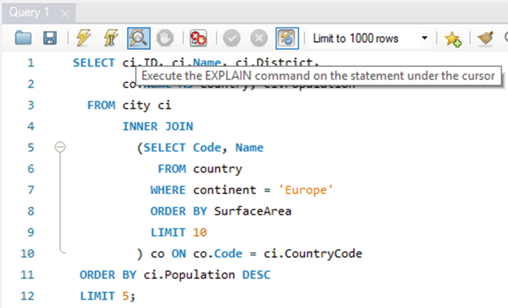
Obtaining the Visual Explain diagram for a query
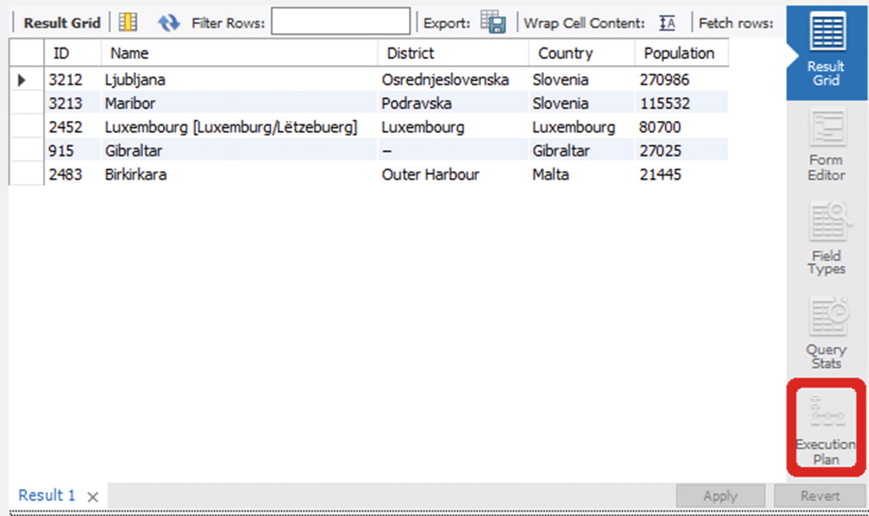
Retrieving the execution plan from the result grid window
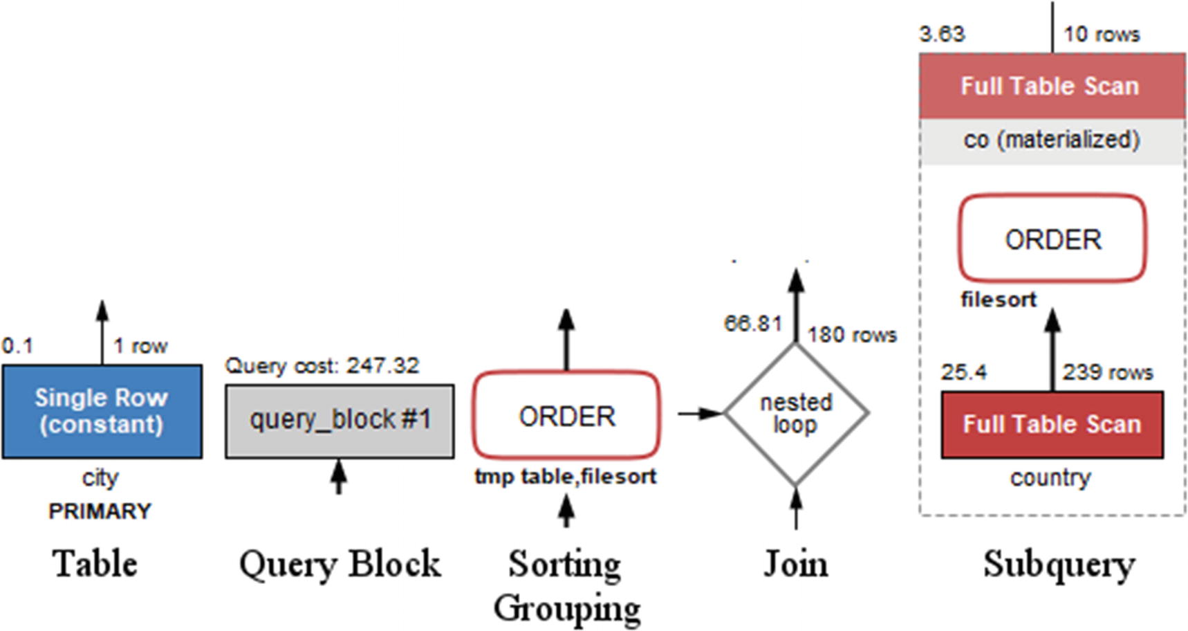
Examples of the shapes used in Visual Explain
In the figure, a query block is gray, while the two examples of a table (the single row lookup and full table scan in the subquery) are blue and red, respectively. The gray blocks are also used, for example, in case of unions. The text below a table box shows the table name or alias in standard text and the index name in bold text. The rectangles with rounded corners depict operations on the rows such as sorting, grouping, distinct operations, and so on.
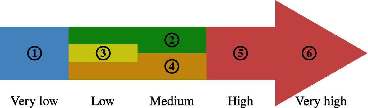
Color codes for the relative cost of operations and table access
Blue (1) is the cheapest; green (2), yellow (3), and orange (4) represent low to medium costs; and the most expensive access types and operations are red symbolizing a high (5) to very high (6) cost.
There is a good deal of overlap between the color groups. Each cost estimate is considering an “average” use case, so the cost estimates should not be taken as an absolute truth. Query optimization is complex, and sometimes a method that is usually cheaper than another method for one particular query turns out to give better performance.
The author of this book once decided to improve a query that had a query plan which looked terrible: internal temporary tables, file sorting, poor access methods, and so on. After a long time rewriting the query and verifying whether the tables had the correct indexes, the query plan looked beautiful – but it turned out the query performed worse than the original. The lesson: Always test the query performance after optimization and do not rely on whether the cost of the access methods and operations has improved on paper.
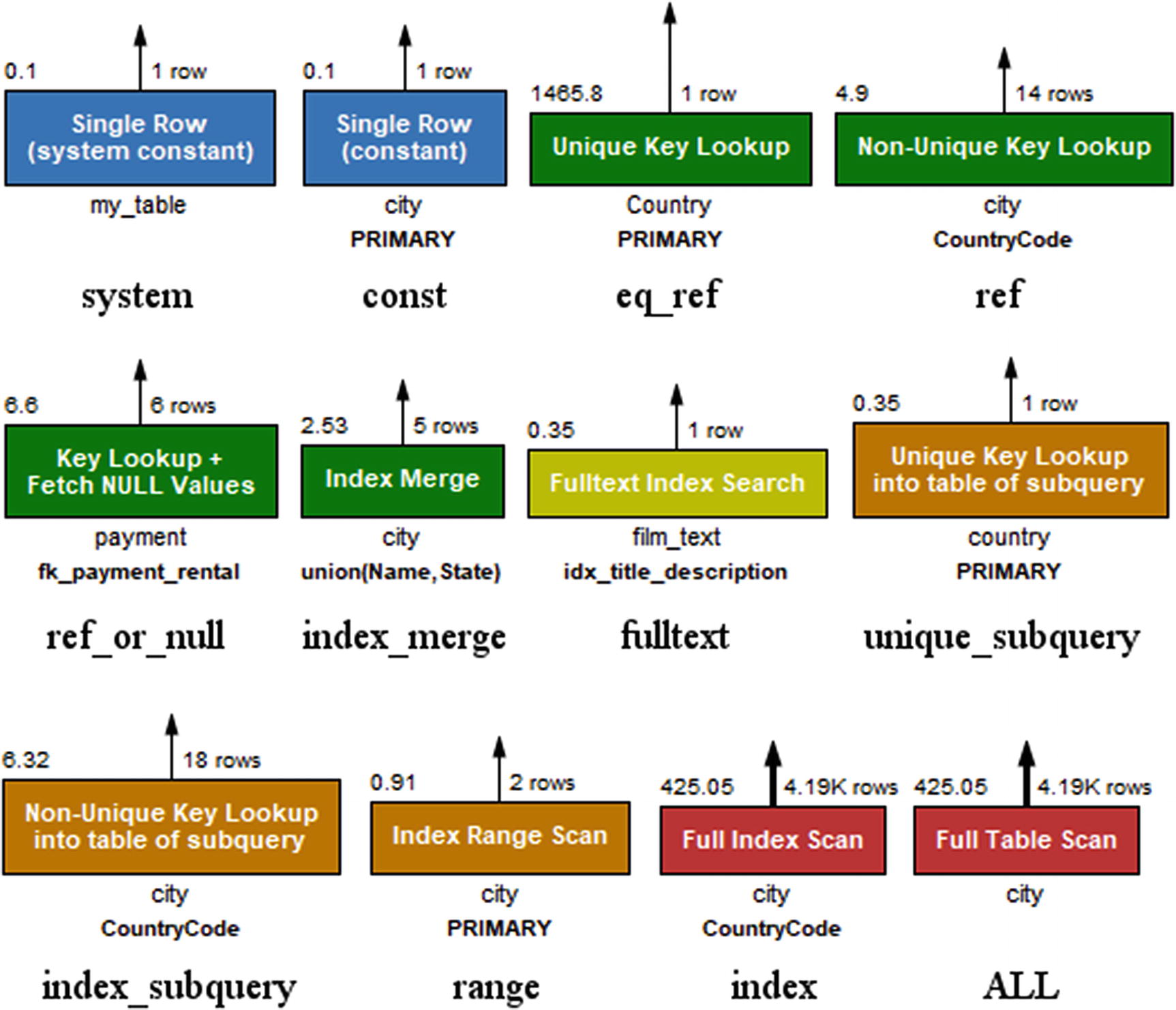
The access types as displayed in Visual Explain
Additionally, Visual Explain has an “unknown” access type colored black in case it comes across an access type that is not known. The access types are ordered from left to right and then top to bottom according to their color and approximate cost.

The Visual Explain diagram for the example query
You read the diagram from the bottom left to the right and then up. So the diagram shows that the subquery with a full table scan on the country table is performed first and then another full table scan on the materialized co table with the rows joined on the ci (city) table using a nonunique index lookup. Finally, the result is sorted using a temporary table and a file sort.
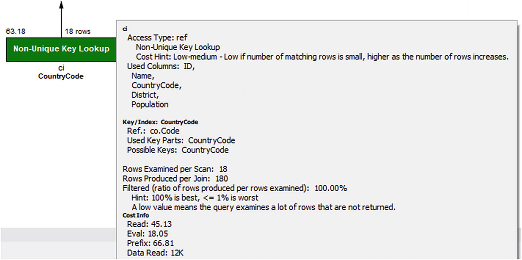
Details for the ci table in Visual Explain
Not only does the pop-up frame show the remaining details that also are available in the JSON output, there are also hints to help understand what the data means. All of this means that Visual Explain is a great way to get started analyzing queries through their query plans. As you gain experience, you may prefer using the text-based outputs, particularly if you prefer to work from a shell, but do not dismiss Visual Explain because you think it is better to use the text-based output format. Even for experts, Visual Explain is a great tool for understanding how queries are executed.
Hopefully, discussing the output formats has given you an idea of what information EXPLAIN can give you. Yet, to fully understand it and take advantage of it, it is necessary to dive deeper into the meaning of the information.
EXPLAIN Output
There is a lot of information available in the explain outputs, so it is worth delving into what this information means. This section starts out with an overview of the fields included in the traditional and JSON-formatted outputs; then the select types and access types and the extra information will be covered in more detail.
EXPLAIN Fields
The first step to use the EXPLAIN statement constructively in your work to improve your queries is to understand what information is available. The information ranges from an id to make a reference to the query parts to details about the indexes that can be used for the query compared to what is used and what optimizer features are applied.
The EXPLAIN fields
Traditional | JSON | Description |
|---|---|---|
id | select_id | A numeric identifier that shows which part of the query the table or subquery is part of. The top-level tables have id = 1, the first subquery has id = 2, and so forth. In case of a union, the id will be NULL with the table value set to <unionM,N> (see also the table column) for the row that represents the aggregation of the union result. |
select_type | This shows how the table will be included in the overall statement. The known select types will be discussed later in the “Select Types” section. For the JSON format, the select type is implied by the structure of the JSON document and from fields such as dependent and cacheable. | |
dependent | Whether it is a dependent subquery, that is, it depends on the outer parts of the query. | |
cacheable | Whether the result of the subquery can be cached or it must be reevaluated for each row in the outer query. | |
table | table_name | The name of the table or subquery. If an alias has been specified, it is the alias that is used. This ensures that each table name is unique for a given value of the id column. Special cases include unions, derived tables, and materialized subqueries where the table name is <unionM,N>, <derivedN>, and <subqueryN>, respectively, where N and M refer to the ids of earlier parts of the query plan. |
partitions | partitions | The partitions that will be included for the query. You can use this to determine whether partition pruning is applied as expected. |
type | access_type | How the data is accessed. This shows how the optimizer has decided to limit the number of rows that are examined in the table. The types will be discussed in the “Access Types” section. |
possible_keys | possible_keys | A list of the indexes that are candidates to be used for the table. A key name using the schema <auto_key0> means an auto-generated index is available. |
key | key | The index(es) chosen for the table. A key name using the schema <auto_key0> means an auto-generated index is used. |
key_len | key_length | The number of bytes that are used of the index. For indexes that consist of multiple columns, the optimizer may only be able to use a subset of the columns. In that case, the key length can be used to determine how much of the index is useful for this query. If the column in the index supports NULL values, 1 byte is added to the length compared to the case of a NOT NULL column . |
used_key_parts | The columns in the index that are used. | |
ref | ref | What the filtering is performed against. This can, for example, be a constant for a condition like <table>.<column> = 'abc' or a name of a column in another table in case of a join. |
rows | rows_examined_per_scan | An estimate of the number of rows that is the result of including the table. For a table that is joined to an earlier table, it is the number of rows estimated to be found per join. A special case is when the reference is the primary key or a unique key on the table, in which case the row estimate is exactly 1. |
rows_produced_per_join | The estimated number of rows resulting from the join. Effectively the number of loops expected multiplied with rows_examined_per_scan and the percentage of rows filtered. | |
filtered | filtered | This is an estimate of how many of the examined rows will be included. The value is in percent, so that for a value of 100.00 all examined rows will be returned. A value of 100.00 is the optimal, and the worst value is 0. Note: The rounding of the value in the traditional format depends on the client you use. MySQL Shell will, for example, return 100 where the mysql command-line client returns 100.00. |
cost_info | A JSON object with the breakdown of the cost of the query part. | |
Extra | Additional information about the decisions of the optimizer. This can include information about the sorting algorithm used, whether a covering index is used, and so on. The most common of the supported values will be discussed in the section “Extra Information.” | |
message | Information that is in the Extra column for the traditional output that does not have a dedicated field in the JSON output. An example is Impossible WHERE . | |
using_filesort | Whether a file sort is used. | |
using_index | Whether a covering index is used. | |
using_temporary_table | Whether an operation such as a subquery or sorting requires an internal temporary table. | |
attached_condition | The WHERE clause associated with the part of the query. | |
used_columns | The columns required from the table. This is useful to see if you are close to be able to use a covering index. |
Some of the information appears at first to be missing in the JSON format as the field only exists for the traditional format. That is not the case; instead the information is available using other means, for example, several of the messages in Extra have their own field in the JSON format. Other Extra messages use the message field. Some of the fields that are not included in the table for the JSON output will be mentioned when discussing the information in the Extra column later in this section.
In general, Boolean fields in the JSON-formatted output are omitted, if the value is false; one exception is for cacheable as a non-cacheable subquery or union indicates a higher cost compared to the cacheable cases.
table: Access a table. This is the lowest level of the operations.
query_block: The highest-level concept with one query block corresponding to an id for the traditional format. All queries have at least one query block.
nested_loop: A join operation.
grouping_operation: The operation, for example, resulting from a GROUP BY clause.
ordering_operation: The operation, for example, resulting for an ORDER BY clause.
duplicates_removal: The operation, for example, resulting when using the DISTINCT keyword.
windowing: The operation resulting from using window functions.
materialized_from_subquery: Execute a subquery and materialize the result.
attached_subqueries: A subquery that is attached to the rest of the query. This, for example, happens with clauses such as IN (SELECT ...) for the subquery inside the IN clause.
union_result: For queries using UNION to combine the result of two or more queries. Inside the union_result block, there is a query_specifications block with the definition of each query in the union.
The fields in Table 20-1 and the list of complex operations are not comprehensive for the JSON format, but it should give you a good idea of the information available. In general, the field names carry information in themselves, and combining with the context where they occur is usually enough to understand the meaning of the field. The values of some of the fields deserve some more attention though – starting with the select types.
Select Types
The select type shows what kind of query block each part of the query is. A part of a query can in this context include several tables. For example, if you have a simple query joining a list of tables but not using constructs such as subqueries, then all tables will be in the same (and only) part of the query. Each part of the query gets each own id (select_id in the JSON output).
EXPLAIN select types
Select Type | JSON | Description |
|---|---|---|
SIMPLE | For SELECT queries not using derived tables, subqueries, unions, or similar. | |
PRIMARY | For queries using subqueries or unions, the primary part is the outermost part. | |
INSERT | For INSERT statements. | |
DELETE | For DELETE statements. | |
UPDATE | For UPDATE statements. | |
REPLACE | For REPLACE statements. | |
UNION | For union statements, the second or later SELECT statement. | |
DEPENDENT UNION | dependent=true | For union statements, the second or later SELECT statement where it depends on an outer query. |
UNION RESULT | union_result | The part of the query that aggregates the results from the union SELECT statements. |
SUBQUERY | For SELECT statements in subqueries. | |
DEPENDENT SUBQUERY | dependent=true | For dependent subqueries, the first SELECT statement. |
DERIVED | A derived table – a table created through a query but otherwise behaves like a normal table. | |
DEPENDENT DERIVED | dependent=true | A derived table dependent on another table. |
MATERIALIZED | materialized_from_subquery | A materialized subquery. |
UNCACHEABLE SUBQUERY | cacheable=false | A subquery where the result must be evaluated for each row in the outer query. |
UNCACHEABLE UNION | cacheable=false | For a union statement, a second or later SELECT statement that is part of an uncacheable subquery. |
Some of the select types can be taken just as information to make it easier to understand which part of the query you are looking at. This, for example, includes PRIMARY and UNION. However, some of the select types indicate that it is an expensive part of the query. This particularly applies to the uncacheable types. Dependent types also mean that the optimizer has less flexibility when deciding where in the execution plan to add the table. If you have slow queries and you see uncacheable or dependent parts, it can be worth looking into whether you can rewrite those parts or split the query into two.
Another important piece of information is how the tables are accessed.
Access Types
The table access types were already encountered when Visual Explain was discussed. They show whether a query accesses the table using an index, scan, and similar. Since the cost associated with each access type varies greatly, it is also one of the important values to look for in the EXPLAIN output to determine which parts of the query to work on to improve the performance.
The rest of this subsection summarizes the access types in MySQL. The headings are the values used in the type column in the traditional format. For each access type, there is an example that uses that access type.
system
Cost: Very low
Message: Single Row (system constant)
Color: Blue
The system access type is a special case of the const access type.
const
Cost: Very low
Message: Single row (constant)
Color: Blue
eq_ref
Cost: Low
Message: Unique key lookup
Color: Green
The eq_ref access type is a specialized case of the ref access type where only one row can be returned per lookup.
ref
Cost: Low to medium
Message: Non-unique key lookup
Color: Green
ref_or_null
Cost: Low to medium
Message: Key lookup + fetch NULL values
Color: Green
index_merge
Cost: Medium
Message: Index merge
Color: Green
While the cost is listed as medium, one of the more common severe performance issues is a query usually using a single index or doing a full table scan and the index statistics becoming inaccurate, so the optimizer chooses an index merge. If you have a poorly performing query using an index merge, try to tell the optimizer to ignore the index merge optimization or the used indexes and see if that helps or analyze the table to update the index statistics. Alternatively, the query can be rewritten to a union of two queries, with each query using a part of the filter. An example of this will be shown in Chapter 24.
fulltext
Cost: Low
Message: Fulltext index search
Color: Yellow
unique_subquery
Cost: Low
Message: Unique key lookup into table of subquery
Color: Orange
The unique_subquery access method is a special case of the index_subquery method for the case where a primary or unique index is used.
index_subquery
Cost: Low
Message: Nonunique key lookup into table of subquery
Color: Orange
range
Cost: Medium
Message: Index range scan
Color: Orange
The cost of using range access largely depends on how many rows are included in the range. In one extreme, the range scan only matches a single row using the primary key, so the cost is very low. In the other extreme, the range scan includes a large part of the table using a secondary index in which case it can end up being cheaper to perform a full table scan.
The range access type is related to the index access type with the difference being whether partial or a full scan is required.
index
Cost: High
Message: Full index scan
Color: Red
Since an index scan requires a second lookup using the primary key, it can become very expensive unless the index is a covering index for the query, to the extent that it ends up being cheaper to perform a full table scan.
ALL
Cost: Very high
Message: Full table scan
Color: Red
If you see a table other than the first table using a full table scan, it is usually a red flag that indicates that either there is a missing condition on the table or there are no indexes that can be used. Whether ALL is a reasonable access type for the first table depends on how much of the table you need for the query; the larger the part of the table is required, the more reasonable a full table scan is.
While a full table scan is considered the most expensive access type, it is together with primary key lookups the cheapest per row. So, if you genuinely need to access most or all of the table, a full table scan is the most effective way to read the rows.
That concludes the discussion of the access types for now. The access types will be referenced again when looking at EXPLAIN examples later in this chapter as well as later in the book when looking at optimizing queries, for example, in Chapter 24. In the meantime, let’s look at the information in the Extra column.
Extra Information
The Extra column in the traditional output format is a catch-all bin for information that does not have its own column. When the JSON format was introduced, there was no reason to keep it as it was easy to introduce additional fields and it is not necessary to include all fields for every output. For that reason, the JSON format does not have an Extra field but instead has a range of fields. A few leftover messages have been left for a generic message field.
The information available in the Extra column is in some cases storage engine dependent or only used in rare cases. This discussion will only cover the most commonly encountered messages. For a full list of messages, refer to the MySQL reference manual at https://dev.mysql.com/doc/refman/en/explain-output.html#explain-extra-information.
Using index: When a covering index is used. For the JSON format, the using_index field is set to true.
Using index condition: When an index is used to test whether it is necessary to read the full row. This is, for example, used when there is a range condition on an indexed column. For the JSON format, the index_condition field is set with the filter condition.
Using where: When a WHERE clause is applied to the table without using an index. This may be an indication that the indexes on the table are not optimal. In the JSON format, the attached_condition field is set with the filter condition.
Using index for group-by: When a loose index scan is used to resolve GROUP BY or DISTINCT. In the JSON format, the using_index_for_group_by field is set to true.
Using join buffer (Block Nested Loop): This means that a join is made where no index can be used, so the join buffer is used instead. Tables with this message are candidates to have an index added. For the JSON format, the using_join_buffer field is set to Block Nested Loop. One thing to be aware of is that when a hash join is used, then the traditional and JSON-formatted outputs will still show that a block nested loop is used. To see whether it is an actual block nested loop join or a hash join, you need to use the tree-formatted output.
Using join buffer (Batched Key Access): This means that a join is using the Batched Key Access (BKA) optimization. To enable the Batched Key Access optimization, you must enable the mrr (defaults to on) and batch_key_access (defaults to off) and disable the mrr_cost_based (defaults to on) optimizer switches. The optimization requires an index for the join, so unlike using the join buffer for a block nested loop, using the Batched Key Access algorithm is not a sign of expensive access to the table. For the JSON format, the using_join_buffer field is set to Batched Key Access.
Using MRR: The Multi-Range Read (MRR) optimization is used. This is sometimes used to reduce the amount of random I/O for range conditions on secondary indexes where the full row is needed. The optimization is controlled by the mrr and mrr_cost_based optimizer switches (both are enabled by default). For the JSON format, the using_MRR field is set to true.
Using filesort: MySQL uses an extra pass to determine how to retrieve the rows in the correct order. This, for example, happens with sorting by a secondary index; and the index is not a covering index. For the JSON format, the using_filesort field is set to true.
Using temporary: An internal temporary table is used to store the result of a subquery, for sorting, or for grouping. For sorting and grouping, the use of an internal temporary table can sometimes be avoided by adding an index or rewriting the query. For the JSON format, the using_temporary_table field is set to true.
sort_union(...), Using union(...), Using intersect(...): These three messages are used with index merges to say how the index merge is performed. For either message, information about the indexes involved in the index merge is included inside the parentheses. For the JSON format, the key field specifies the method and indexes used.
Recursive: The table is part of a recursive common table expression (CTE). For the JSON format, the recursive field is set to true.
Range checked for each record (index map: 0x1): This happens when you have a join where there is a condition on an indexed column of the second table that depends on the value of a column from the first table, for example, with an index on t2.val2: SELECT * FROM t1 INNER JOIN t2 WHERE t2.val2 < t1.val1; This is what triggers the NO_GOOD_INDEX_USED counter in the Performance Schema statement event tables to increment. The index map is a bitmask that indicates which indexes are candidates for the range check. The index numbers are 1-based as shown by SHOW INDEXES. When you write out the bitmask, the index numbers with the bit set are the candidates. For the JSON format, the range_checked_for_each_record field is set to the index map.
Impossible WHERE: When there is a filter that cannot possibly be true, for example, WHERE 1 = 0. This also applies if the value in the filter is outside the range supported by the data type, for example, WHERE ID = 300 for a tinyint data type. For the JSON format, the message is added to the message field.
Impossible WHERE noticed after reading const tables: The same as Impossible WHERE except it applies after resolving the tables using the system or const access method. An example is SELECT * FROM (SELECT 1 AS ID) a INNER JOIN city USING (ID) WHERE a.id = 130; For the JSON format, the message is added to the message field.
Impossible HAVING: The same as Impossible WHERE except it applies to a HAVING clause. For the JSON format, the message is added to the message field.
Using index for skip scan: When the optimizer chooses to use multiple range scans similar to a loose index scan. It can, for example, be used for a covering index where the first column of the index is not used for the filter condition. This method is available in MySQL 8.0.13 and later. For the JSON format, the using_index_for_skip_scan field is set to true.
Select tables optimized away: This message means that MySQL was able to remove the table from the query because only a single row will result, and that row can be generated from a deterministic set of rows. It usually occurs when only the minimum and/or maximum values of an index are required from the table. For the JSON format, the message is added to the message field.
No tables used: For subqueries that do not involve any tables, for example, SELECT 1 FROM dual; For the JSON format, the message is added to the message field.
no matching row in const table: For a table where the system or const access type is possible but there are no rows matching the condition. For the JSON format, the message is added to the message field.
At the time of writing, you need to use the tree-formatted output to see if a join that does not use indexes is using the hash join algorithm.
That concludes the discussion about the meaning of the output of the EXPLAIN statement. All there is left is to start using it to examine the query plans.
EXPLAIN Examples
To finish off the discussion of query plans, it is worth going through a few examples to get a better feeling of how you can put all of it together. The examples here are meant as an introduction. Further examples will occur in the remainder of the book, particularly Chapter 24.
Single Table, Table Scan
The EXPLAIN output for a single table with a table scan
The output has the access type set to ALL which is also what would be expected since there are no conditions on columns with indexes. It is estimated that 4188 rows will be examined (the actual number is 4079) and for each row a condition from the WHERE clause will be applied. It is expected that 10% of the rows examined will match the WHERE clause (note that depending on the client used, the output for the filtered column may say 10 or 10.00). Recall from the optimizer discussion in Chapter 17 that the optimizer uses default values to estimate the filtering effect of various conditions, so you cannot use the filtering value directly to estimate whether an index is useful.
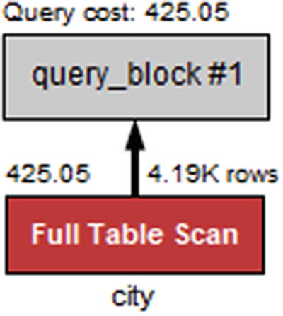
Visual Explain diagram for a single table with a table scan
The full table scan is shown by a red Full Table Scan box, and it can be seen that the cost is estimated to be 425.05.
This query just returns two rows (the table has a London in England and one in Ontario, Canada). What happens if all cities in a single country are requested instead?
Single Table, Index Access
The EXPLAIN output for a single table with index lookups
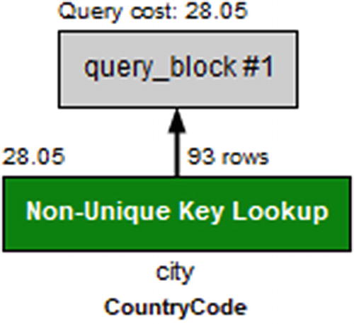
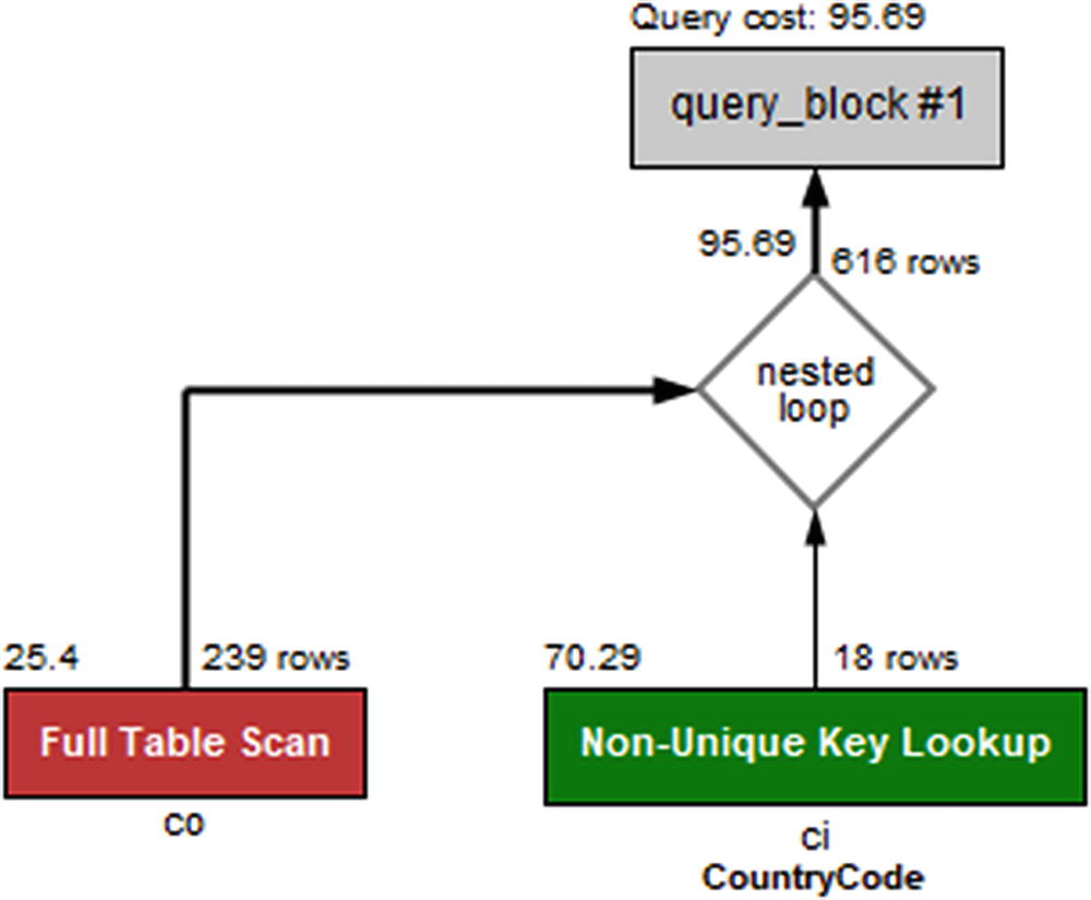
Visual Explain diagram for a single table with index lookup
Despite returning more than 45 times as many rows as the first example, the cost is only estimated as 28.05 or less than one-tenth of the cost of a full table scan.
What happens if only the ID and CountryCode columns are used?
Two Tables and a Covering Index
The EXPLAIN output for a simple join between two tables
Visual Explain diagram for a simple join between two tables
The key_len field does not include the primary key part of the index even though it is used. It is however useful to see how much of a multicolumn index is used.
Multicolumn Index
The EXPLAIN output using part of a multicolumn index
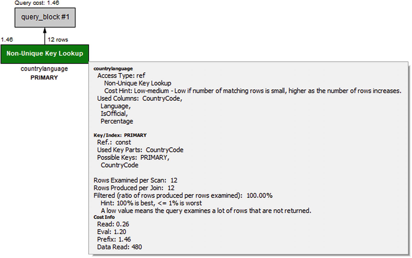
Visual Explain diagram for using part of a multicolumn index
In the figure, look for the Used Key Parts label under Key/Index: PRIMARY. This directly shows that only the CountryCode column of the index is used.
As a final example, let’s return to the query that was used as an example when going through the EXPLAIN formats.
Two Tables with Subquery and Sorting
The example query that has been used extensively earlier in the chapter will be used to round off the discussion about EXPLAIN. The query uses a mix of various features, so it triggers several parts of the information that has been discussed. It is also an example of a query with multiple query blocks. As a reminder, the query is repeated here.
The EXPLAIN output when joining a subquery and a table
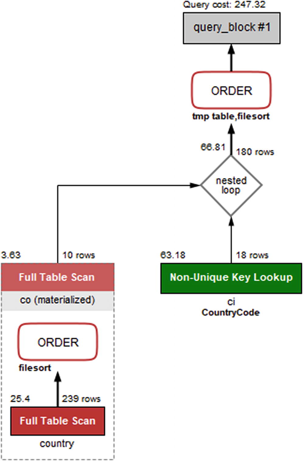
Visual Explain diagram for joining a subquery and a table
The query plan starts out with the subquery that uses the country table to find the ten smallest countries by area. The subquery is given the table label <derived2>, so you will need to find the row (could be several rows for other queries) with id = 2 which is row 3 in this case. Row 3 has the select type set to DERIVED, so it is a derived table; that is a table created through a query but otherwise behaves like a normal table. The derived table is generated using a full table scan (type = ALL) with a WHERE clause applied to each row, followed by a file sort. The resulting derived table is materialized (visible from Visual Explain) and called co.
Once the derived table has been constructed, it is used as the first table for the join with the ci (city) table. You can see that from the ordering of the rows with <derived2> in row 1 and ci in row 2. For each row in the derived table, it is estimated that 18 rows will be examined in the ci table using the CountryCode index. The CountryCode index is a nonunique index which can be seen from the label for the table box in Visual Explain, and the type column has the value ref. It is estimated that the join will return 180 rows which comes from the ten rows in the derived table multiplied with the estimate of 18 rows per index lookup in the ci table.
Finally, the result is sorted using an internal temporary table and a file sort. The total cost of the query is estimated to be 247.32.
Thus far, the discussion has been on what the query plan ended up being. If you want to know how the optimizer got there, you will need to examine the optimizer trace.
Optimizer Trace
The optimizer trace is not needed very often, but sometimes when you encounter an unexpected query plan, it can be useful to see how the optimizer got there. That is what the optimizer trace shows.
Most often when a query plan is not what you expect, it is because of a missing or wrong WHERE clause, a missing or wrong join condition, or some other kind of error in the query or because the index statistics are not correct. Check these things before diving into the gory details of the optimizer’s decision process.
The optimizer trace is enabled by setting the optimizer_trace option to 1. This makes the optimizer record the trace information for the subsequent queries (until optimizer_trace is disabled again), and the information is made available through the information_schema.OPTIMIZER_TRACE table. The maximum number of traces that are retained is configured with the optimizer_trace_limit option (defaults to 1).
- 1.
Enable the optimizer_trace option for the session.
- 2.
Execute EXPLAIN for the query you want to investigate.
- 3.
Disable the optimizer_trace option again.
- 4.
Retrieve the optimizer trace from the information_schema.OPTIMIZER_TRACE table.
QUERY: The original query.
TRACE: A JSON document with the trace information. There will be more about the trace shortly.
MISSING_BYTES_BEYOND_MAX_MEM_SIZE: The size (in bytes) of the recorded trace is limited to the value of the optimizer_trace_max_mem_size option (defaults to 1 MiB in MySQL 8). This column shows how much more memory is required to record the full trace. If the value is greater than 0, increase the optimizer_trace_max_mem_size option with that amount.
INSUFFICIENT_PRIVILEGES: Whether you were missing privileges to generate the optimizer trace.
The table is created as a temporary table, so the traces are unique to the session.
Obtaining the optimizer trace for a query
The optimizer trace for choosing the access type for the ci table
This shows that it is estimated that on average a little more than 18 rows will be examined when using the CountryCode index ("access_type": "ref") with a cost of 63.181. For the full table scan ("access_type": "scan"), it is expected that it will be necessary to examine 4188 rows with a total cost of 4194.3. The "chosen" element shows that the ref access type has been chosen.
While it is rarely necessary to delve into the details of how the optimizer arrived at the query plan, it can be useful to learn about how the optimizer works. Occasionally, it can also be useful to see the estimated cost of other options for the query plan to understand why they are not chosen.
If you are interested in learning more about using the optimizer traces, you can read more in the MySQL internals manual at https://dev.mysql.com/doc/internals/en/optimizer-tracing.html.
Thus far, the whole discussion – except for EXPLAIN ANALYZE – has been about analyzing the query at the stage before it is executed. If you want to examine the actual performance, EXPLAIN ANALYZE is usually the best option. Another option is to use the Performance Schema.
Performance Schema Events Analysis
The Performance Schema allows you to analyze how much time is spent on each of the events that are instrumented. You can use that to analyze where time is spent when a query is executed. This section will examine how you can use the Performance Schema to analyze a stored procedure to see which of the statements in the procedure take the longest and how to use the stage events to analyze a single query. At the end of the section, it will be shown how you can use the sys.ps_trace_thread() procedure to create a diagram of work done by a thread and how you can use the ps_trace_statement_digest() to collect statistics for statements with a given digest.
Examining a Stored Procedure
It can be challenging to examine the work done by a stored procedure as you cannot use EXPLAIN directly on the procedure and it may not be obvious which queries will be executed by the procedure. Instead you can use the Performance Schema. It records each statement executed and maintains the history in the events_statements_history table .
Unless you need to store more than the last ten queries per thread, you do not need to do anything to start the analysis. If the procedure generates more than ten statement events, you will need to either increase the value of the performance_schema_events_statements_history_size option (requires a restart), use the events_statements_history_long table, or use the sys.ps_trace_thread() procedure as explained later. The remaining part of this discussion assumes you can use the events_statements_history table.
An example procedure
The procedure executes three queries. The first query sets the v_id variable to an integer between 1 and 4079 (the available ID values in the world.city table). The second query fetches the name for the city with that id. The third query finds all cities with the same name as was found in the second query.
The output of the procedure is random, so will differ for each execution. You can then use the thread id found with the PS_CURRENT_THREAD_ID() function (use sys.ps_thread_id(NULL) in MySQL 8.0.15 and earlier) to determine which queries were executed.
Analyzing the queries executed by a stored procedure
The analysis consists of two queries. The first determines the overall information for the procedure which is done by querying for the latest occurrence (sorting by EVENT_ID) of the statement/sql/call_procedure event which is the event for calling a procedure.
The second query asks for the events for the same thread that has the event id of the statement/sql/call_procedure event as the nesting event id. These are the statements executed by the procedure. By ordering by EVENT_ID, the statements are returned in the order they are executed.
The query result of the second query shows that the procedure starts out with four SET statements. Some of these are expected, but there are also some that are triggered by implicitly setting variables. The last two rows are the most interesting for this discussion as they show that two queries were executed. First, the city table is queried by its ID column (the primary key). As expected, it examines one row. Because the result is saved in the v_name variable, the ROWS_AFFECTED counter is incremented instead of ROWS_SENT.
The second query does not perform as well. It also queries the city table but by name where there is no index. This results in 4080 rows being examined to return a single row. The NO_INDEX_USED column is set to 1 to reflect that a full table scan was performed.
One disadvantage of using this approach to examine stored procedures is that – as you can see – it can quickly use all ten rows in the history table. One alternative is to enable the events_statements_history_long consumer and test the procedure on an otherwise idle test system or disable history logging for the other connections. This allows you to analyze procedures executing up to 10000 statement events. An alternative is to use the sys.ps_trace_thread() procedure which also uses the long history but supports polling while the procedure is executing, so it can collect the events even if the table is not large enough to hold all events for the duration of the procedure.
This example has been using the statement events to analyze the performance. Sometimes you need to know what happens at a finer-grained level in which case you need to start looking at the stage events.
Analyzing Stage Events
If you need to get finer-grained details of where a query spends time, the first step is to look at the stage events. Optionally, you can also include wait events. Since the step to work with wait events is essentially the same as for stage events, it is left as an exercise for the reader to analyze the wait events for a query.
The finer-grained the events you examine, the more overhead they will have. Thus, be careful enabling stage and wait events on production systems. Some wait events, particularly related to mutexes, may also impact the query enough that they affect the conclusions of the analysis. Using wait events to analyze a query is usually something only performance architects and developers working with the MySQL source code need to do.
Finding the stages for the last statement of a connection
The event id, the stage name (removing the two first parts of the full event name for brevity), and the latency formatted with the FORMAT_PICO_TIME() function (use the sys.format_time() function in MySQL 8.0.15 and earlier) are selected from the events_stages_history_long table. The WHERE clause filters on the thread id of the connection that executed the query and by the nesting event id. The nesting event id is set to the event id of the latest executed statement for the connection with thread id equal to 83. The result shows that the slowest part of the query is Sending data which is the stage where the storage engine finds and sends the rows.
The main issue analyzing queries this way is that you are either limited by the ten events per thread saved by default or you risk the events being expunged from the long history table before you are done examining it. The sys.ps_trace_thread() procedure was created to help with that problem.
Analysis with the sys.ps_trace_thread( ) Procedure
When you need to analyze a complex query or a stored program executing more than a few statements, you can benefit from using a tool that automatically collects the information as the execution progresses. An option to do this from the sys schema is the ps_trace_thread() procedure.
The procedure loops for a period of time polling the long history tables for new transactions, statements, stages, and wait events. Optionally, the procedure can also set up the Performance Schema to include all events and enable the consumers to record the events. However, since it is usually too much to include all events, it is recommended to set up the Performance Schema yourself to instrument and consume the events that are of interest for your analysis.
Another optional feature is to reset the Performance Schema tables at the start of the monitoring. This can be great if it is acceptable to remove the content of the long history tables.
Thread ID: The Performance Schema thread id that you want to monitor.
Out File: A file to write the result to. The result is created using the dot graph description language.2 This requires that the secure_file_priv option has been set to allow writing files to the target directory and the file does not exist and the user executing the procedure has the FILE privilege.
Max Runtime: The maximum time to monitor in seconds. There is support for specifying the value with 1/100 of a second precision. If the value is set to NULL, the runtime is set to 60 seconds.
Poll Interval: The interval between polling the history tables. The value can be set with the precision of 1/100 of a second. If the value is set to NULL, then the polling interval will be set to one second.
Refresh: A Boolean whether to reset the Performance Schema tables used for the analysis.
Auto Setup: A Boolean whether to enable all instruments and consumers that can be used by the procedure. When enabled, the current settings are restored when the procedure completes.
Debug: A Boolean whether to include additional information such as where in the source code the event is triggered. This is mostly useful when including wait events.
Using the ps_trace_thread() procedure
In this example, only the events_statements_history_long consumer is enabled. This will allow to record all the statement events that result for calling the testproc() procedure as it was done manually earlier. The thread id that will be monitored is obtained using the PS_CURRENT_THREAD_ID() function (in MySQL 8.0.15 and earlier, use sys.ps_thread_id(NULL)).
The ps_trace_thread() procedure is invoked for thread id 32 with the output written to /mysql/files/thread_32.gv. The procedure polls every 0.1 second for 10 seconds, and all the optional features are disabled.
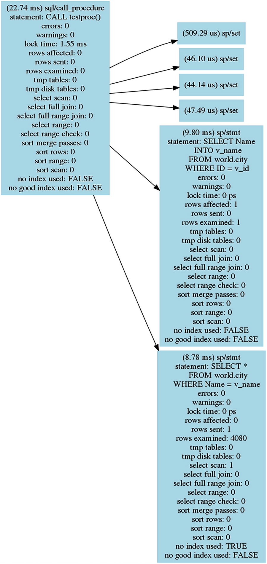
The statement graph for the CALL testproc() statement
The statement graph includes the same information as when the procedure was analyzed manually. For a procedure as simple as testproc(), the advantage of generating the graph is limited, but for more complex procedures or for analyzing queries with lower-level events enabled, it can be a good way to visualize the flow of the execution.
Another sys schema procedure that can help you analyze queries is the ps_trace_statement_digest() procedure.
Analysis with the ps_trace_statement_digest( ) Procedure
As a final example of using the Performance Schema to analyze queries, the ps_trace_statement_digest() procedure from the sys schema will be demonstrated. It takes a digest and then monitors the events_statements_history_long and events_stages_history_long tables for events related to statements with that digest. The result of the analysis includes summary data as well as details such as the query plan for the longest-running query.
Digest: The digest to monitor. Statements will be monitored irrespective of the default schema if their digest matches the one provided.
Runtime: How long to monitor for in seconds. No decimals are allowed.
Poll Interval: The interval between polling the history tables. The value can be set with the precision of 1/100 of a second and must be less than 1 second.
Refresh: A Boolean whether to reset the Performance Schema tables used for the analysis.
Auto Setup: A Boolean whether to enable all instruments and consumers that can be used by the procedure. When enabled, the current settings are restored when the procedure completes.
It may vary from execution to execution which of these queries is the slowest.
Using the ps_trace_statement_digest() procedure
The output starts out with the summary for all the queries found during the analysis. A total of 13 executions were detected using a total of 7.29 milliseconds. The overall summary also includes the aggregates for the time spent for various stages. The next part of the output are the details for the slowest of the 13 executions. The output concludes with the JSON-formatted query plan for the slowest of the queries.
There is a limitation you should be aware of for generating the query plan. The EXPLAIN statement will be executed with the default schema set to the same as where the procedure executed. That means that if the query is executed in a different schema and it does not use a fully qualified table name (i.e., including the schema name), then the EXPLAIN statement will fail, and the procedure does not output the query plan.
Summary
This chapter has covered how you can analyze queries that you believe may need optimization. The bulk of the chapter focused on the EXPLAIN statement that is the main tool for analyzing queries. The remainder of the chapter went through optimizer traces and how to use the Performance Schema to analyze queries.
The EXPLAIN statement supports several different formats that help you get the query plan in the format that works best for you. The traditional format uses a standard table output, the JSON format returns a detailed JSON document, and the tree format shows a relatively simple tree of the execution. The tree format is only supported in MySQL 8.0.16 and later and requires that the Volcano iterator executor is used to execute the query. The JSON format is what the Visual Explain feature in MySQL Workbench uses to create diagrams of the query plan.
There is a vast amount of information available about the query plan in the EXPLAIN outputs. The fields of the traditional format as well as the most commonly encountered fields of JSON were discussed. This included discussing the select types and access types and the extra information in detail. Finally, a series of examples were used to show how this information can be used.
The optimizer traces can be used to get information on how the optimizer ended up with the query plan that the EXPLAIN statement returned. It is usually not necessary to use the optimizer traces for end users, but they can be useful to learn more about the optimizer and the decision process that leads to the query plans.
The final part of the chapter showed how you can use the Performance Schema events to determine what is taking the time for a statement. It was first shown how you can break a stored procedure into individual statements and then how a statement can be broken into stages. Finally the ps_trace_thread() procedure was used to automate the analysis and create a graph of the events, and the ps_trace_statement_digest() procedure was used to collect statistics for a given statement digest.
This chapter analyzed queries. It is sometimes necessary to take the whole transaction into account. The next chapter will show how you can analyze transactions.