
From time to time, it is necessary to perform schema changes or to import large amount of data into a table. This may be to accommodate a new feature, restore a backup, import data generated by a third-party process, or similar. While the raw disk write performance is naturally very important, there are also several things you can do on the MySQL side to improve the performance of these operations.
If you have problems that restoring your backups takes too long, consider switching to a backup method that copies the data files directly (a physical backup) such as using MySQL Enterprise Backup. A major benefit of physical backups is that they are much faster to restore than a logical backup (containing the data as INSERT statement or in a CSV file).
This chapter starts out discussing schema changes and then moves on to some general considerations around loading data. These considerations also apply when you insert single rows at a time. The rest of the chapter covers how to improve the data load performance from inserting in primary key order, how the buffer pool and secondary indexes impact performance, configuration, and tweaking the statements themselves. Finally, the parallel import feature of MySQL Shell is demonstrated.
Schema Changes
When you need to perform changes to your schema, it can require a large amount of work for the storage engine, possibly involving making a completely new copy of the table. This section will go into what you can do to speed up this process starting with the algorithms supported for schema changes and followed by other considerations such as the configuration.
While OPTIMIZE TABLE does not make any changes to the schema of the table, InnoDB implements it as an ALTER TABLE followed by ANALYZE TABLE. So the discussion in this section also applies to OPTIMIZE TABLE.
Algorithm
MySQL supports several algorithms for ALTER TABLE with the algorithm deciding how the schema change is performed. Some schema changes can be made “instantly” by changing the table definitions, while at the other end of the spectrum some changes require copying the entire table into a new table.
INSTANT: Changes are only made to the table definition. While the change is not quite instant, it is very fast. The INSTANT algorithm is available in MySQL 8.0.12 and later.
INPLACE: Changes are in general made within the existing tablespace file (the tablespace id does not change), but with some exceptions such as ALTER TABLE <table name> FORCE (used by OPTIMIZE TABLE) which is more like the COPY algorithm but allowing concurrent data changes. This may be a relatively cheap operation but may also involve copying all the data.
COPY: The existing data is copied to a new tablespace file. This is the algorithm with the most impact as it typically requires more locks, causes more I/O, and takes longer.
Adding a new column as the last column in the table.
Adding a generated virtual column.
Dropping a generated virtual column.
Setting a default value for an existing column.
Dropping the default value for an existing column.
Changing the list of values allowed for a column with the enum or set data type. A requirement is that the storage size does not change for the column.
Changing whether the index type (e.g., BTREE) is set explicitly for an existing index.
The row format cannot be COMPRESSED.
The table cannot have a full text index.
Temporary tables are not supported.
Tables in the data dictionary cannot use the INSTANT algorithm.
If you, for example, need to add a column to an existing table, make sure to add it as the last column, so it can be added “instantly.”
Performance wise, an in-place change is usually – but not always – faster than a copying change. Furthermore, when a schema change is made online (LOCK=NONE), InnoDB must keep track of the changes made during the execution of the schema change. This adds to the overhead, and it takes time to apply the changes that were made during the schema change at the end of the operation. If you are able to take a shared (LOCK=SHARED) or exclusive lock (LOCK=EXCLUSIVE) on the table, you can in general get better performance compared to allowing concurrent changes.
Other Considerations
Since the work done by an in-place or copying ALTER TABLE is very disk intensive, the single biggest effect on performance is how fast the disks are and how much other write activity there is during the schema change. This means that from a performance perspective, it is best to choose to perform schema changes that require copying or moving a large amount of data when there is little to no other write activity on the instance and host. This includes backups which on their own can be very I/O intensive.
You can monitor the progress of ALTER TABLE and OPTIMIZE TABLE for InnoDB tables using the Performance Schema. The simplest way is to use the sys.session view and look at the progress column which has the approximate progress in percentage of the total work. The feature is enabled by default.
If your ALTER TABLE includes creating or rebuilding secondary indexes (this includes OPTIMIZE TABLE and other statements rebuilding the table), you can use the innodb_sort_buffer_size option to specify how much memory each sort buffer can use. Be aware that a single ALTER TABLE will create multiple buffers, so be careful not to set the value too large. The default value is 1 MiB, and the maximum allowed value is 64 MiB. A larger buffer may in some cases improve the performance.
When you create full text indexes, then you can use the innodb_ft_sort_pll_degree option to specify how many threads InnoDB will use to build the search index. The default is 2 with supported values between 1 and 32. If you are creating full text indexes on large tables, it may be an advantage to increase the value of innodb_ft_sort_pll_degree.
One special DDL operation that needs consideration is to drop or truncate a table.
Dropping or Truncating Tables
It may seem unnecessary to have to consider performance optimizations of dropping tables. It would seem that all that is required is to delete the tablespace file and remove references to the table. In practice, it is not quite so simple.
Disabling the adaptive hash index will make queries benefitting from the hash index run slower, but for tables with a size of a couple of hundred gigabytes or larger, a relatively small slowdown from disabling the adaptive hash index is usually preferred over potential stalls occurring because of the overhead of removing references to the table that is being dropped or truncated.
That concludes the discussion of performing schema changes. The rest of the chapter discusses loading data.
General Data Load Considerations
Before discussing how to improve the performance of bulk inserts, it is worth performing a small test and discussing the result. In the test, 200,000 rows are inserted into two tables. One of the tables has an auto-increment counter as the primary key, and the other uses a random integer for the primary key. The row size is identical for the two tables.
The discussion in this and the next section applies equally well to non-bulk inserts.
Python program to map the LSN age of InnoDB pages
The page number, log sequence number, and page type are extracted at the positions (in bytes) defined by the FIL_PAGE_OFFSET, FIL_PAGE_LSN, and FIL_PAGE_TYPE constants for each page. If the page type has the value of the FIL_PAGE_TYPE_ALLOCATED constant, it means it is not used yet, so it can be skipped – these pages are colored black in the log sequence number map.
If you want to explore the information available in the page headers, the file storage/innobase/include/fil0types.h (https://github.com/mysql/mysql-server/blob/8.0/storage/innobase/include/fil0types.h) in the source code and the descriptions of the fil headers in the MySQL internals manual (https://dev.mysql.com/doc/internals/en/innodb-fil-header.html) are good starting points.
You can get help to use the program by invoking it with the --help argument. The only required argument is the path to the tablespace file you want to analyze. Unless, you have set the innodb_page_size option to something else than 16384 bytes, then the default values for the optional arguments are all you need unless you want to change the dimensions and size of the generated map.
Do not use the program on a production system! There is minimal error checking in the program to keep it as simple as possible, and it is experimental in nature.
Populating a table with an auto-incrementing primary key
The output of the program shows there are 880 pages in the tablespace plus possibly some unused pages at the end of the file.
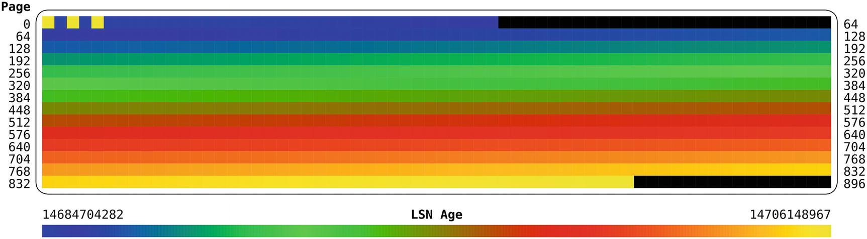
The LSN age for each page when inserting in primary key order
In the figure, the top left represents the first pages of the tablespace. As you go through the figure from left to right and top to bottom, the pages are further and further into the tablespace file, and the lower right represents the last pages. The figure shows that other than the first pages, the pattern of the age of the pages follows the same pattern as in the LSN Age scale at the bottom of the figure. This means that the age of the pages becomes younger as you progress through the tablespace. The first few pages are the exception as they, for example, include the tablespace header.
This pattern shows that the data is sequentially inserted into the tablespace making it as compact as possible. It also makes it as likely as possible that if a query reads data from several pages that are logical in sequence, then they are also physical in sequence in the tablespace file.
Populating a table with a random primary key

The LSN age for each page when inserting in random order
This time the log sequence number age pattern is completely different. The age colors for all pages except the unused pages correspond to the colors for the most recent log sequence numbers. That means all of the pages with data were last updated around the same time, or in other words they are all written to until the end of the bulk load. The number of pages with data is 1345 compared to the 880 pages used in the table with the auto-increment primary key. That is more than 50% more pages.
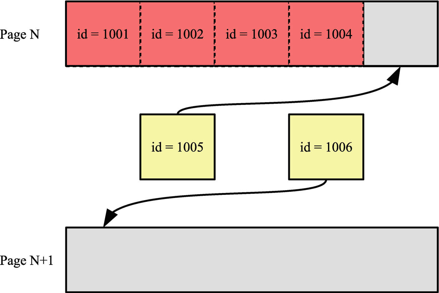
Example of adding a new row when inserting in sequential order
The figure shows two new rows being inserted. The row with id = 1005 can just fit into page N, so when the row with id = 1006 is inserted, it is inserted into the next page. Everything is nice and compact in this scenario.
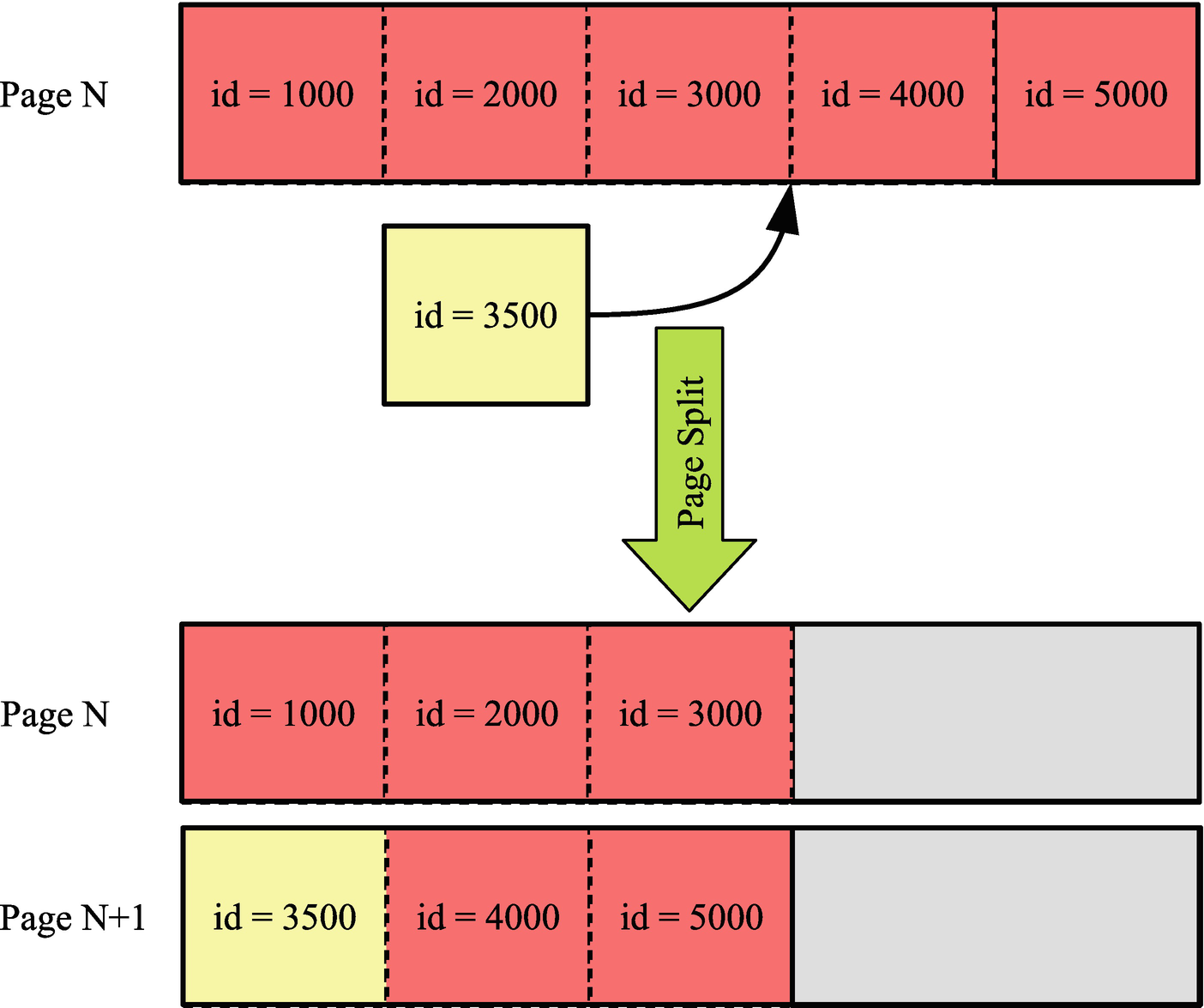
Example of a page split as result of inserting in random order
In this case the row with id = 3500 is inserted, but there is no more room in page N where it logically belongs. So page N is split into pages N and N+1 with roughly half the data going into each page.
There are two immediate consequences of the page split. First, the data that previously occupied one page now uses two pages which is why the insert in random order ends up occupying 50% more pages which also means the same data requires more space in the buffer pool. A significant side effect of the additional pages is that the B-tree index ends up with more leaf pages and potentially more levels in the tree, and given that each level in the tree means an extra seek when accessing the page, this causes additional I/O.

Example of the location of pages on the disk
In the figure three extents are depicted. For simplicity, just five pages are shown in each extent (with the default page size of 16 KiB, there are 64 pages per extent). Pages that have been part of page splits are highlighted. Page 11 was split at a time when the only later page was page 13, so pages 11 and 12 are still located relatively close. Page 15, however, was split when several extra pages had been created meaning page 16 ended up in the next extent.
The combination of deeper B-trees, more pages that take up space in the buffer pool, and more random I/O means that the performance of a table where rows are inserted in random primary key order will not be as good as for an equivalent table with data inserted in primary key order. The performance difference not only applies to inserting the data; it also applies to subsequent uses of the data. For this reason, it is important for optimal performance to insert the data in primary key order. How you can achieve that is discussed next.
Insert in Primary Key Order
As the previous discussion showed, there are great advantages of inserting the data in primary key order. The easiest way to achieve that is to auto-generate the primary key values by using an unsigned integer and declaring the column for auto-incrementing. Alternatively, you will need to ensure yourself that the data is inserted in the primary key order. This section will investigate both cases.
Auto-increment Primary Key
The simplest way to ensure data is inserted in the primary key order is to allow MySQL to assign the values itself by using an auto-increment primary key. You do that by specifying the auto_increment attribute for the primary key column when creating the table. It is also possible to use an auto-increment column in connection with a multicolumn primary key; in that case, the auto-increment column must be the first column in the index.
Creating tables with an auto-increment primary key
The t1 table just has a single column for the primary key, and the value is auto-incrementing. The reason for using an unsigned integer instead of a signed integer is that auto-increment values are always greater than 0, so using an unsigned integer allows twice as many values before exhausting the available values. The examples use a 4 byte integer which allows for a little less than 4.3 billion rows if all values are used. If that is not enough, you can declare the column as bigint unsigned which uses 8 bytes and allows for 1.8E19 rows.
The t2 table adds a datetime column to the primary key which, for example, can be useful if you want to partition by the time the row is created. The auto-incrementing id column still ensures the rows are created with a unique primary key, and because the id column is the first in the primary keys, rows are still inserted in primary key order even if subsequent columns in the primary key are random in nature.
Using the sys.schema_auto_increment_columns view
You can see from the output that the table uses a smallint unsigned column for the auto-increment values which has a maximum value of 65535, and the column is named payment_id. The next auto-increment value is 16049, so 24.49% of the available values are used.
In case you insert data from an external source, you may already have values assigned for the primary key column (even when using an auto-increment primary key). Let’s look at what you can do in that case.
Inserting Existing Data
Whether you need to insert data generated by some process, restore a backup, or convert a table using a different storage engine, it is best to ensure that it is in primary key order before inserting it. If you generate the data or it already exists, then you can consider sorting the data before inserting it. Alternatively, use the OPTIMIZE TABLE statement to rebuild the table after the import has completed.
The rebuild may take a substantial amount of time for large tables, but the process is online except for short durations at the start and end where locks are needed to ensure consistency.
If you create a backup using the mysqldump program, you can add the --order-by-primary option which makes mysqldump add an ORDER BY clause that includes the columns in the primary key (mysqlpump does not have an equivalent option). This is particularly useful if the backup is created of tables using a storage engine that uses so-called heap organized data such as MyISAM with the purpose of restoring it to an InnoDB table (using an index organization of the data).
While you should not in general rely on the order rows are returned when using a query without an ORDER BY clause, InnoDB’s index-organized rows mean that a full table scan will usually (but no guarantees) return the rows in primary key order even if you omit the ORDER BY clause. A noticeable exception is when the table includes a secondary index covering all columns and the optimizer chooses to use that index for the query.
Ordering data by the primary key when copying it
As a final case, consider when you have a UUID as the primary key.
UUID Primary Keys
If you are limited to a UUID for your primary key, for example, because you cannot change the application to support an auto-increment primary key, then you can improve the performance by swapping the UUID components around and storing the UUIDs in a binary column.
A UUID (MySQL uses UUID version 1) consists of a timestamp as well as a sequence number (to guarantee uniqueness if the timestamp moves backward, e.g., during daylight savings changes) and the MAC address.
In some cases, it may be considered a security issue to reveal the MAC address as it can be used to identify the computer and potentially the user.
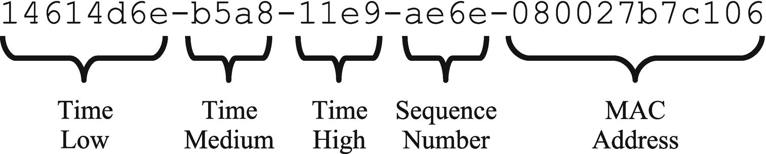
The five parts of a UUID version 1
The low part of the timestamp represents up to 4,294,967,295 (0xffffffff) intervals of 100 nanoseconds or just under 430 seconds. That means that every seven minutes and a little less than 10 seconds, the low part of the timestamp rolls over making the UUID start over from an ordering point of view. This is why plain UUIDs do not work well for the index-organized data as it means the inserts will largely be into a random place in the primary key tree.
Using the UUID_TO_BIN() and BIN_TO_UUID() functions
The advantage of this approach is twofold. Because the UUID has the low and high time components swapped, it becomes monotonically increasing making it much more suitable for the index-organized rows. The binary storage means that the UUID only requires 16 bytes of storage instead of 36 bytes in the hex version with dashes to separate the parts of the UUID. Remember that because the data is organized by the primary key, the primary key is added to secondary indexes so it is possible to go from the index to the row, so the fewer bytes required to store the primary key, the smaller the secondary indexes.
InnoDB Buffer Pool and Secondary Indexes
The single most important factor for the performance of bulk data loads is the size of the InnoDB buffer pool. This section discusses why the buffer pool is important for bulk data loads.
When you insert data into a table, InnoDB needs to be able to store the data in the buffer pool until the data has been written to the tablespace files. The more data you can store in the buffer pool, the more efficiently InnoDB can perform the flushing of dirty pages to the tablespace files. However, there is also a second reason which is maintaining the secondary indexes.
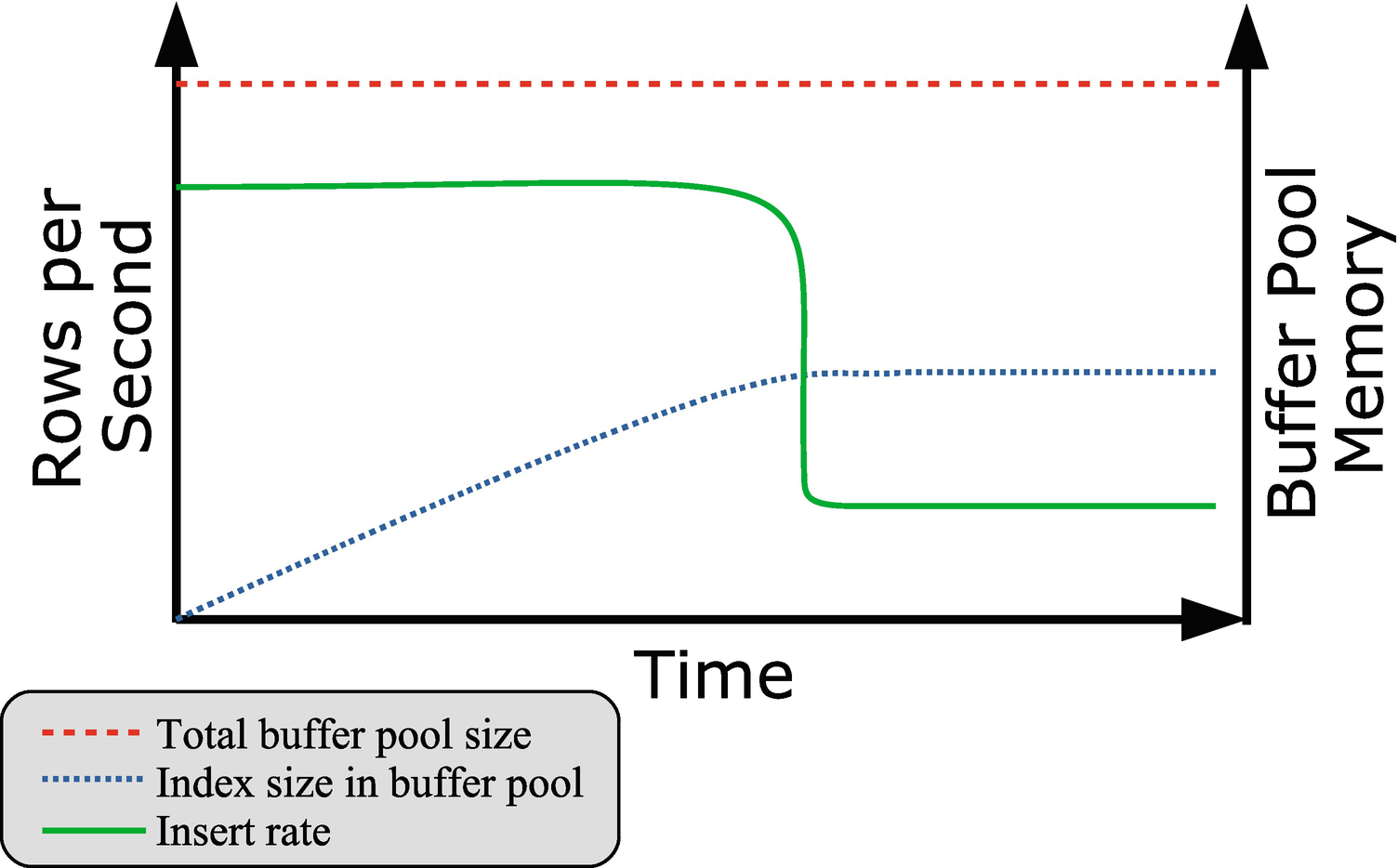
Insert performance compared to the index size in the buffer pool
The figure shows how the insert rate is roughly constant for a while and during that period more and more of the buffer pool is used for secondary indexes. When no more of the index can be stored in the buffer pool, the insert rate suddenly drops off. In the extreme case of loading data into a table with a single secondary index that includes the whole row with nothing else going on, the drop comes when the secondary index uses close to half the buffer pool (and the remaining for the primary key).
The result will depend on how much you have used the index, so in general your result will be different. The query is best used on a test system as there can be a significant overhead querying the INNODB_BUFFER_PAGE table .
Be careful querying the INNODB_BUFFER_PAGE table on your production system as the overhead can be significant, particularly if you have a large buffer pool with many tables and indexes in it.
Increase the size of the buffer pool.
Remove the secondary indexes while inserting data.
Partition the table.
Once the data load has completed, you can set the buffer pool size back to the usual value (134217728 if you use the default).
If you are inserting into an empty table, a very useful strategy is to remove all the secondary indexes (possibly leaving unique indexes for the data validation) before loading the data and then add the indexes back. This is in most cases more efficient than trying to maintain the indexes while loading the data, and it is also what the mysqlpump utility does if you use that to create backups.
The last of the strategies is to partition the table. This helps as the indexes are local to the partition (this is the reason the partition key must be part of all unique indexes), so if you insert the data in the partition order, InnoDB will only have to maintain the indexes for the data in the current partition. That makes each index smaller, so they easier fit into the buffer pool.
Configuration
You can influence the load performance through the configuration of the session that performs the load. This includes considering switching off constraint checks, how auto-increment ids are generated, and more.
Configuration options influencing the data load performance
Option Name | Scope | Description |
|---|---|---|
foreign_key_checks | Session | Specifies whether to check if the new rows violate the foreign keys. Disabling this option can improve performance for tables with foreign keys. |
unique_checks | Session | Specifies whether to check if the new rows violate unique constraints. Disabling this option can improve performance for tables with unique indexes. |
innodb_autoinc_lock_mode | Global | Specifies how InnoDB determines the next auto-increment values. Setting this option to 2 (the default in MySQL 8 – requires binlog_format = ROW) gives the best performance at the expense of potentially nonconsecutive auto-increment values. Requires restarting MySQL. |
innodb_flush_log_at_trx_commit | Global | Determines how frequently InnoDB flushes changes made to the data files. If you import data using many small transactions, setting this option to 0 or 2 can improve the performance. |
sql_log_bin | Session | Disables the binary log when set to 0 or OFF. This will greatly reduce the amount of data written. |
transaction_isolation | Session | Sets the transaction isolation level. If you are not reading existing data in MySQL, consider setting the isolation level to READ UNCOMMITTED. |
All of the options have side effects, so consider carefully whether changing the setting is appropriate for you. For example, if you are importing data from an existing instance to a new instance, and you know there are no problems with foreign key and unique key constraints, then you can disable the foreign_key_checks and unique_checks options for the session importing the data. If you are on the other hand importing from a source, where you are not sure of the data integrity, it may be better to keep the constraint checks enabled to ensure the quality of the data even if it means a slower load performance.
For the innodb_flush_log_at_trx_commit option , you need to consider whether a risk of losing the last second or so of committed transactions is acceptable. If your data load process is the only transactions on the instance, and it is easy to redo the import, you can set innodb_flush_log_at_trx_commit to 0 or 2 to reduce the number of flushes. The change is mostly useful with small transactions. If the import commits less than once a second, there is very little gained by the change. If you change innodb_flush_log_at_trx_commit, then remember to set the value back to 1 after the import.
For the binary log, it is useful to disable writing the imported data as it greatly reduces the amount of data changes that must be written to disk. This is particularly useful if the binary log is on the same disk as the redo log and data files. If you cannot modify the import process to disable sql_log_bin, you can consider restarting MySQL with the skip-log-bin option to disable the binary log altogether, but note that will also affect all other transactions on the system. If you do disable binary logging during the import, it can be useful to create a full backup immediately after the import, so you can use the binary logs for point-in-time recoveries again.
If you use replication, consider doing the data import separately on each instance in the topology with sql_log_bin disabled. Please note though that it will only work when MySQL does not generate auto-increment primary keys and is only worth the added complexity if you need to import a large amount of data. For the initial load in MySQL 8.0.17, you can just populate the source of the replication and use the clone plugin3 to create the replica.
You can also improve the load performance by the statements you choose to import the data and how you use transactions.
Transactions and Load Method
A transaction denotes a group of changes, and InnoDB will not fully apply the changes until the transaction is committed. Each commit involves writing the data to the redo logs and includes other overheads. If you have very small transactions – like inserting a single row at a time – this overhead can significantly affect the load performance.
There is no golden rule for the optimal transaction size. For small row sizes, usually a few thousand rows are good, and for larger row sizes choose fewer rows. Ultimately, you will need to test on your system and with your data to determine the optimal transaction size.
For the load method, there are two main choices: INSERT statements or the LOAD DATA [LOCAL] INFILE statement. In general LOAD DATA performs better than INSERT statements as there is less parsing. For INSERT statements, it is an advantage of using the extended insert syntax where multiple rows are inserted using a single statement rather than multiple single-row statements.
When you use mysqlpump for your backups, you can set the --extended-insert option to the number of rows to include per INSERT statement with the default being 250. For mysqldump, the --extended-insert option works as a switch. When it is enabled (the default), mysqldump will decide on the number of rows per statement automatically.
An advantage of using LOAD DATA to load the data is also that MySQL Shell can automate doing the load in parallel.
MySQL Shell Parallel Load Data
One problem you can encounter when you load data into MySQL is that a single thread cannot push InnoDB to the limit of what it can sustain. If you split the data into batches and load the data using multiple threads, you can increase the overall load rate. One option to do this automatically is to use the parallel data load feature of MySQL Shell 8.0.17 and later.
The parallel load feature is available through the util.import_table() utility in Python mode and the util.importTable() method in JavaScript mode. This discussion will assume you are using Python mode. The first argument is the filename, and the second (optional) argument is a dictionary with the optional arguments. You can get the help text for the import_table() utility using the util.help() method, like
mysql-py> util.help('import_table')
The help text includes a detailed description of all the settings that can be given through the dictionary specified in the second argument.
MySQL Shell disables duplicate key and foreign key checks and sets the transaction isolation level to READ UNCOMMITTED for the connection doing the import to reduce the overhead during the import as much as possible.
Using the util.import_table() utility with default settings
The warning when creating the chapter_25 schema depends on whether you have created the schema earlier. Notice that you must enable the local_infile option for the utility to work.
The most interesting part of the example is the execution of the import. When you do not specify anything, MySQL Shell splits the file into 50 MB chunks and uses up to eight threads. In this case the file is 85.37 MB (MySQL Shell uses the metric file sizes – 85.37 MB is the same as 81.42 MiB), so it gives two chunks, of which the first is 50 MB and the second 35.37 MB. That is not a terrible good distribution.
You must enable local_infile on the server side before invoking the util.import_table() utility.
Using util.import_table() with several custom settings
In this case the target schema, table, and columns are specified explicitly, and the file is split into four roughly equal chunks and the number of threads is set to four. The format of the CSV file is also included in the setting (the specified values are the default).
The optimal number of threads varies greatly depending on the hardware, the data, and the other queries running. You will need to experiment to find the optimal settings for your system.
Summary
This chapter has discussed what determines the performance of DDL statements and bulk data loads. The first topic was schema changes in terms of ALTER TABLE and OPTIMIZE TABLE. There is support for three different algorithms when you make schema changes. The best-performing algorithm is the INSTANT algorithm which can be used to add columns at the end of the row and several metadata changes. The second-best algorithm is INPLACE which in most cases modifies the data within the existing tablespace file. The final, and in general most expensive, algorithm is COPY.
In cases where the INSTANT algorithm cannot be used, there will be a substantial amount of I/O, so the disk performance is important, and the less other work going on requiring disk I/O, the better. It may also help to lock the table, so MySQL does not need to keep track of data changes and apply them at the end of the schema change.
For inserting data, it was discussed that it is important to insert in primary key order. If the insert order is random, it leads to larger tables, a deeper B-tree index for the clustered index, more disk seeks, and more random I/O. The simplest way to insert data in primary key order is to use an auto-increment primary key and let MySQL determine the next value. For UUIDs, MySQL 8 adds the UUID_TO_BIN() and BIN_TO_UUID() functions that allow you to reduce the storage required for a UUID to 16 bytes and to swap the low and high order parts of the timestamp to make the UUIDs monotonically increasing.
When you insert data, a typical cause of the insert rate suddenly slowing down is when the secondary indexes no longer fit into the buffer pool. If you insert into an empty table, it is an advantage to remove the indexes during the import. Partitioning may also help as it splits the index into one part per partition, so only part of the index is required at a time.
In some circumstances, you can disable constraint checks, reduce flushing of the redo log, disable binary logging, and reduce the transaction isolation to READ UNCOMMITTED. These configuration changes will all help reduce the overhead; however, all also have side effects, so you must consider carefully whether the changes are acceptable for your system. You can also affect the performance by adjusting the transaction size to balance the reduction of commit overhead and overhead of working with large transactions.
For bulk inserts you have two options of loading the data. You can use regular INSERT statements, or you can use the LOAD DATA statement. The latter is in general the preferred method. It also allows you to use the parallel table import feature of MySQL Shell 8.0.17 and later.
In the next chapter, you will learn about improving the performance of replication.