
When you encounter a performance problem, the first step is to determine what is causing it. There may be several causes for poor performance, so you should keep an open mind when looking for causes. The focus of this chapter is to find queries that may contribute to the poor performance or that may become a problem in the future when the load and amount of data increase. Still, as discussed in Chapter 1, you need to consider all aspects of your system, and often it may turn out to be a combination of factors that causes the problem.
This chapter goes through the various sources of query performance–related information. First, the Performance Schema will be discussed. The Performance Schema is the basis for many of the other features discussed in this chapter. Second, the views of the sys schema are covered as well as the statement performance analyzer feature. Third, it is shown how you can use MySQL Workbench as a way to get a graphical user interface for several of the reports discussed in the first two sections. Fourth, it is discussed how monitoring is important to find candidates for optimization. While the section uses MySQL Enterprise Monitor as the basis of the discussion, the principles apply to monitoring in general, so you are encouraged to read the section even if you use a different monitoring solution. Fifth and final is the slow query log which is the traditional tool for finding slow queries.
This chapter includes several examples with outputs. In general, your output for the same example will differ for values that include timings and other data that is not deterministic.
Queries that perform poorly due to lock contention will not be covered; instead, Chapter 22 goes into detail on how to investigate lock issues. Transactions are covered in Chapter 21.
The Performance Schema
The Performance Schema is a gold mine for information about the performance of your queries. This makes it the obvious place to start when discussing how to find queries that are candidates for optimization. You may likely end up using some of the methods that build on top of the Performance Schema, but you are still encouraged to get a good understanding of the underlying tables, so you know how to access the raw data and make your own custom reports.
This section will start out discussing how to get information about the statements and prepared statement, then table and file I/O are covered, and finally it is shown how to find out what are causing errors and which errors.
The Statement Event Tables
Using the Performance Schema tables based on statement events is the most straightforward way to look for queries that are candidates for optimization. These tables will allow you to get very detailed information about the queries that are executing on the instance. One important thing to note is that queries executed as prepared statements are not included in the statement tables.
events_statements_current: The statements currently executing or for idle connections the latest executed query. When executing stored programs, there may be more than one row per connection.
events_statements_history: The last statements for each connection. The number of statements per connection is capped at performance_schema_events_statements_history_size (defaults to 10). The statements for a connection are removed when the connection is closed.
events_statements_history_long: The latest queries for the instance irrespective of which connection executed it. This table also includes statements from connections that have been closed. The consumer for this table is disabled by default. The number of rows is capped at performance_schema_events_statements_history_long_size (defaults to 10000).
events_statements_summary_by_digest: The statement statistics grouped by the default schema and digest. This table is discussed in detail later.
events_statements_summary_by_account_by_event_name: The statement statistics grouped by the account and event name. The event name shows what kind of statement is executed, for example, statement/sql/select for a SELECT statement executed directly (not executed through a stored program).
events_statements_summary_by_host_by_event_name: The statement statistics grouped by the hostname of the account and the event name.
events_statements_summary_by_program: The statement statistics grouped by the stored program (event, function, procedure, table, or trigger) that executed the statement. This is useful to find the stored programs that perform the most work.
events_statements_summary_by_thread_by_event_name: The statement statistics grouped by thread and event name. Only threads currently connected are included.
events_statements_summary_by_user_by_event_name: The statement statistics grouped by the username of the account and the event name.
events_statements_summary_global_by_event_name: The statement statistics grouped by the event name.
events_statements_histogram_by_digest: Histogram statistics grouped by the default schema and digest.
events_statements_histogram_global: Histogram statistics where all queries are aggregated in one histogram.
threads: Information about all threads in the instance, both background and foreground threads. You can use this table instead of the SHOW PROCESSLIST command. In addition to the process list information, there are columns showing whether the thread is instrumented, the operating system thread id, and more.
The columns in the events_statements_summary_by_digest table
Column Name | Description |
|---|---|
SCHEMA_NAME | The schema that was the default schema when executing the query. If no schema was the default, the value is NULL. |
DIGEST | The digest of the normalized query. In MySQL 8, that is a sha256 hash. |
DIGEST_TEXT | The normalized query. |
COUNT_STAR | The number of times the query has been executed. |
SUM_TIMER_WAIT | The total amount of time that has been spent executing the query. Note that the value flows over after a little more than 30 weeks of execution time. |
MIN_TIMER_WAIT | The fastest the query has been executed. |
AVG_TIMER_WAIT | The average execution time. This is the same as SUM_TIMER_WAIT/COUNT_STAR unless SUM_TIMER_WAIT has overflown. |
MAX_TIMER_WAIT | The slowest the query has been executed. |
SUM_LOCK_TIME | The total amount of time that has been spent waiting for table locks. |
SUM_ERRORS | The total number of errors that have been encountered executing the query. |
SUM_WARNINGS | The total number of warnings that have been encountered executing the query. |
SUM_ROWS_AFFECTED | The total number of rows that have been modified by the query. |
SUM_ROWS_SENT | The total number of rows that have been returned (sent) to the client. |
SUM_ROWS_EXAMINED | The total number of rows that have been examined by the query. |
SUM_CREATED_TMP_DISK_TABLES | The total number of on-disk internal temporary tables that have been created by the query. |
SUM_CREATED_TMP_TABLES | The total number of internal temporary tables – whether created in memory or on disk – that have been created by the query. |
SUM_SELECT_FULL_JOIN | The total number of joins that have performed full table scans as there is no index for the join condition or there is no join condition. This is the same that increments the Select_full_join status variable. |
SUM_SELECT_FULL_RANGE_JOIN | The total number of joins that use a full range search. This is the same that increments the Select_full_range_join status variable. |
SUM_SELECT_RANGE | The total number of times the query has used a range search. This is the same that increments the Select_range status variable. |
SUM_SELECT_RANGE_CHECK | The total number of joins by the query where the join does not have an index that checks for the index usage after each row. This is the same that increments the Select_range_check status variable. |
SUM_SELECT_SCAN | The total number of times the query has performed a full table scan on the first table in the join. This is the same that increments the Select_scan status variable. |
SUM_SORT_MERGE_PASSES | The total number of sort merge passes that have been done to sort the result of the query. This is the same that increments the Sort_merge_passes status variable. |
SUM_SORT_RANGE | The total number of times a sort was done using ranges. This is the same that increments the Sort_range status variable. |
SUM_SORT_ROWS | The total number of rows sorted. This is the same that increments the Sort_rows status variable. |
SUM_SORT_SCAN | The total number of times a sort was done by scanning the table. This is the same that increments the Sort_scan status variable. |
SUM_NO_INDEX_USED | The total number of times no index was used to execute the query. |
SUM_NO_GOOD_INDEX_USED | The total number of times no good index was used. This means that the Extra column in the EXPLAIN output includes “Range checked for each record.” |
FIRST_SEEN | When the query was first seen. When the table is truncated, the first seen value is also reset. |
LAST_SEEN | When the query was seen the last time. |
QUANTILE_95 | The 95th percentile of the query latency. That is, 95% of the queries complete in the time given or in less time. |
QUANTILE_99 | The 99th percentile of the query latency. |
QUANTILE_999 | The 99.9th percentile of the query latency. |
QUERY_SAMPLE_TEXT | An example of a query before it is normalized. You can use this to get the query execution plan for the query. |
QUERY_SAMPLE_SEEN | When the example query was seen. |
QUERY_SAMPLE_TIMER_WAIT | How long the example query took to execute. |
There is a unique index on (SCHEMA_NAME, DIGEST ) which is used to group the data. There can be up to performance_schema_digests_size (dynamically sized, but usually defaults to 10000) rows in the table. When the last row is inserted, the schema and digest are both set to NULL, and that row is used as a catch-all row. Each time the catch-all row is used, the Performance_schema_digest_lost status variable is incremented. The information that is aggregated in this table is also available for individual queries using the events_statements_current, events_statements_history, and events_statements_history_long tables.
Since the data is grouped by SCHEMA_NAME, DIGEST, you get most out of the events_statements_summary_by_digest table, when the application is consistent about setting the default schema (e.g., use world or the --schema command-line option in MySQL Shell or equivalent in the client/connector you use). Either always set it or never set it. In the same way, if you sometimes include the schema name when referencing tables and sometimes do not, then otherwise identical queries will be counted as two different digests.
Two groups of columns need a little more explanation, the quantile columns and the query sample columns. The values of the quantile columns are determined based on histogram statistics for the digests. Basically, if you take the events_statements_histogram_by_digest table for a given digest and default schema and go to the bucket with 95% of the query executions, then that bucket is used to determine the 95th percentile. The histogram tables will be discussed shortly.
It is the first time the digest is encountered for the given default schema.
A new occurrence of the digest and schema has a higher value for TIMER_WAIT than the query currently used as the sample query (i.e., it was slower).
If the value of the performance_schema_max_digest_sample_age option is greater than 0 and the current sample query is older than performance_schema_max_digest_sample_age seconds.
The value of performance_schema_max_digest_sample_age defaults to 60 seconds, which works well if you monitor the events_statements_summary_by_digest table every minute. That way, the monitoring Agent will be able to pick up the slowest query in each one-minute interval and get a complete history of the slowest queries. If your monitoring interval is greater, consider increasing the value of performance_schema_max_digest_sample_age.
As you can see from the list of columns, there are ample opportunities to query for statements meeting some requirements. The trick is to query for the things that are important. What qualifies as important depends on the situation, so it is not possible to give specific queries that will apply to all situations. For example, if you know from your monitoring that there are problems with a large number of internal temporary tables using memory or disk, then the SUM_CREATED_TMP_DISK_TABLES and SUM_CREATED_TMP_TABLES columns are good candidates for filtering.
A large amount of examined rows compared to the number of rows sent back to the client or that are modified. This may suggest poor index usage.
The sum of no index used or no good index used is high. This may suggest that the query can benefit from new indexes or rewriting the query.
The number of full joins is high. This suggests that either an index is needed or there is a join condition missing.
The number of range checks is high. This may suggest that you need to change the indexes on the tables in the query.
If the quantile latencies are showing a severe degradation when going toward higher quantiles, it may suggest you at times have problems resolving the queries in a timely fashion. This may be due to the instance in general being overloaded, lock issues, some conditions triggering poor query plans, or other reasons.
The number of internal temporary tables created in disk is high. This may suggest that you need to consider which indexes are used for sorting and grouping, the amount of memory allowed to internal temporary tables, or other changes that can prevent writing the internal temporary table to disk or create internal temporary tables in the first place.
The number of sort merges is high. This may suggest this query can benefit from a larger sort buffer.
The number of executions is large. This does not suggest any problems with the query, but the more often a query is executed, the more impact improvements of the query have. In some cases, a high execute count may also be caused by unnecessary executions of the query.
The number of errors or warnings is high. While this may not impact the performance, it suggests something is wrong. Do note that some queries always generate a warning, for example, EXPLAIN as it uses warnings to return additional information.
Be careful increasing the value of sort_buffer_size if you are still using MySQL 5.7 as it can decrease performance even if it reduces the number of sort merges. In MySQL 8, the sort buffer has been improved, and the performance degradation of a larger buffer is much less. Still, do not increase the size more than you need.
You should be aware that just because a query meets one of these conditions does not mean there is anything to change. As an example, consider a query that aggregates data from a table. That query may examine large parts of the table but only returns a few rows. It may even require a full table scan where there is no meaningful index that can help. The query will perform badly from the point of view of the ratio between the number of examined rows and the number of sent rows, and maybe the no index counter is incrementing. Yet, the query may very well do the minimum amount of work required to return the required result. If you determine the query is a performance problem, you will need to find a different solution than adding indexes; for example, you may be able to execute the query during non-peak periods and cache the result, or you may have a separate instance where queries like this are executed.
Using the events_statements_summary_by_digest table
The output shows that querying the city table in the world schema by name is the most executed query. You should compare the value COUNT_STAR to other queries to understand how often this query is executed compared to other queries. In this example, you can see that the query on average returns 1.3 rows per execution but examines 4079 rows. That means the query examines more than 3000 rows for each row returned. Since this is an often-executed query, that suggests that an index is needed on the Name column that is used for filtering. The bottom of the output shows an actual example of the query that you can use with EXPLAIN as described in the next chapter to analyze the query execution plan.
As mentioned, MySQL also maintains histogram statistics for the statements. There are two histogram tables available: events_statements_histogram_by_digest and events_statements_histogram_global. The difference between the two is that the former has the histogram information grouped by default schema and digest, whereas the latter contains information for all queries grouped together. The histogram information can be useful to determine the distribution of query latencies, similar to what has been discussed for the quantile columns in the events_statements_summary_by_digest table but more fine-grained. The tables are managed automatically.
As mentioned, prepared statements are not included in the statement event tables. Instead, you need to use the prepared_statements_instances table.
Prepared Statements Summary
Prepared statements can be useful to speed up execution of queries that are reused within a connection. For example, if you have an application that keeps using the same connection(s), then you can prepare the statements the application uses and then execute the prepared statement when it is needed.
Prepared statements use placeholders, so you only need to submit the template of the query when you prepare it. That way you can submit different parameters for each execution. When used in that way, prepared statements serve as a catalogue of statements that the application can use with the parameters needed for a given execution.
Example of using prepared statements
The SQL interface uses user variables to pass the statement and values to MySQL. The first step is to prepare the statement; then it can be used as many times as needed passing the parameters required for the query. Finally, the prepared statement is deallocated.
Using the prepared_statements_instances table
The main differences from the events statements tables are that there are no quantile statistics and query example and the primary key is the OBJECT_INSTANCE_BEGIN – that is, the memory address of the prepared statement instead of a unique key on the default schema and digest. In fact, the default schema and digest are not even mentioned in the prepared_statements_instances table.
As it is hinted by the primary key being the memory address of the prepared statement, the prepared statement statistics are only maintained while the prepared statement exists. So, when the statement is deallocated either explicitly or implicitly because the connection is closed, the statistics are cleared.
That ends the discussion of statement statistics. There are also higher-level statistics such as the table I/O summaries.
Table I/O Summaries
The table I/O information in the Performance Schema is often misunderstood. The I/O that is referred to for the table I/O summaries is a general concept of input-output related to the table. Thus, it does not refer to disk I/O. Rather, it is a general measure of how busy the table is. That said, the more disk I/O there is for a table, the more time will also be spent on table I/O.
table_io_waits_summary_by_table: The aggregate information for the table with details of read, write, fetch, insert, and update I/O.
table_io_waits_summary_by_index_usage: The same information as for the table_io_waits_summary_by_table table except the statistics are per index or lack thereof.
The groups of latencies for table and index I/O statistics
Group | Columns | Descriptions |
|---|---|---|
Overall | COUNT_STAR SUM_TIMER_WAIT MIN_TIMER_WAIT AVG_TIMER_WAIT MAX_TIMER_WAIT | The statistics for the whole table or index. |
Reads | COUNT_READ SUM_TIMER_READ MIN_TIMER_READ AVG_TIMER_READ MAX_TIMER_READ | The aggregate statistics for all read operations. Currently there is only one read operation, fetch, so the read statistics will be the same as the fetch statistics. |
Writes | COUNT_WRITE SUM_TIMER_WRITE MIN_TIMER_WRITE AVG_TIMER_WRITE MAX_TIMER_WRITE | The aggregate statistics for all write operations. The write operations are inserts, updates, and deletes. |
Fetches | COUNT_FETCH SUM_TIMER_FETCH MIN_TIMER_FETCH AVG_TIMER_FETCH MAX_TIMER_FETCH | The statistics for fetching records. The reason this is not called “select” is that records may be fetched for other purposes than for SELECT statements. |
Inserts | COUNT_INSERT SUM_TIMER_INSERT MIN_TIMER_INSERT AVG_TIMER_INSERT MAX_TIMER_INSERT | The statistics for inserting records. |
Updates | COUNT_UPDATE SUM_TIMER_UPDATE MIN_TIMER_UPDATE AVG_TIMER_UPDATE MAX_TIMER_UPDATE | The statistics for updating records. |
Deletes | COUNT_DELETE SUM_TIMER_DELETE MIN_TIMER_DELETE AVG_TIMER_DELETE MAX_TIMER_DELETE | The statistics for deleting records. |
Example of using the table_io_waits_summary_by_table table
In this output, there is a broad usage of the table except rows have not been deleted. It can also be seen that most of the time is spent on reading data (122703207563448 picoseconds out of a total of 125987200409940 picoseconds – or 97%).
Example of using the table_io_waits_summary_by_index_usage table
Consider the three values of COUNT_STAR. If you sum those, 20004 + 549000 + 417489729 = 418058733, you get the same value as COUNT_STAR in the table_io_waits_summary_by_table table. This example shows the same data but split out across the two indexes on the city table as well as the NULL index, which means that no index was used. This makes the table_io_waits_summary_by_index_usage table very useful to estimate the usefulness of the indexes and whether table scans are executed for the table.
By Primary Key: Using the primary key to locate the rows, for example, WHERE ID = 130
By Secondary Index: Using the CountryCode index to locate the rows, for example, WHERE CountryCode = 'AUS'
By No Index: Using a full table scan to locate the rows, for example, WHERE Name = 'Sydney'
The effect of various queries on the table I/O counters
Query/Index | Rows | Reads | Writes |
|---|---|---|---|
SELECT by primary key PRIMARY | 1 | FETCH: 1 | |
SELECT by secondary index CountryCode | 14 | FETCH: 14 | |
SELECT by no index NULL | 1 | FETCH: 4079 | |
UPDATE by primary key PRIMARY | 1 | FETCH: 1 | UPDATE: 1 |
UPDATE by secondary index CountryCode | 14 | FETCH: 15 | UPDATE: 14 |
UPDATE by no index PRIMARY NULL | 1 | FETCH: 4080 | UPDATE: 1 |
DELETE by primary key PRIMARY | 1 | FETCH: 1 | DELETE: 1 |
DELETE by secondary index CountryCode | 14 | FETCH: 15 | DELETE: 14 |
DELETE by no index PRIMARY NULL | 1 | FETCH: 4080 | DELETE: 1 |
INSERT NULL | 1 | INSERT: 1 |
A key takeaway from the table is that for UPDATE and DELETE statements, there are still reads even though they are write statements. The reason is that the rows still must be located before they can be changed. Another observation is that when using the secondary index or no index for updating or deleting rows, then one more record is read than matches the condition. Finally, inserting a row counts as a non-index operation.
When you see a monitoring graph showing a spike in I/O latencies – whether it is table or file I/O – it can be tempting to make the conclusion that there is a problem. Before you do that, take a step back and consider what the data means.
An increase in I/O latencies measured from the Performance Schema is neither a good nor a bad thing. It is a fact. It means that something was doing I/O, and if there is a spike it means there was more I/O during that period than usual, but otherwise you cannot make conclusions from the event on its own.
A more useful way to use this data is in case a problem is reported. This can be that the system administrator reports the disks are 100% utilized or that end users report the system is slow. Then, you can go and look at what happened. If the disk I/O was unusually high at that point in time, then that is likely related, and you can continue your investigation from there. If the I/O is on the other hand normal, then the high utilization is likely caused by another process than MySQL, or a disk in the disk array is being rebuilt, or similar.
Using the information in the table_io_waits_summary_by_table and table_io_waits_summary_by_index_usage tables, you can determine which tables are the most used for the various workloads. For example, if you have one table that is particularly busy with writes, you may want to consider moving its tablespace to a faster disk. Before taking such as a decision, you should also consider the actual file I/O.
File I/O
Unlike the table I/O that has just been discussed, the file I/O statistics are for the actual disk I/O involved with the various files that MySQL uses. This is a good supplement to the table I/O information.
events_waits_summary_global_by_event_name: This is a summary table grouped by the event names. By querying event names starting with wait/io/file/, you can get I/O statistics grouped by the type of I/O. For example, I/O caused by reading and writing the binary log files uses a single event (wait/io/file/sql/binlog). Note that events set to wait/io/table/sql/handler correspond to the table I/O that has just been discussed; including the table I/O allows you to easily compare the time spent on file I/O with the time spent on table I/O.
file_summary_by_event_name: This is similar to the events_waits_summary_global_by_event_name table but just including file I/O and with the events split into reads, writes, and miscellaneous.
file_summary_by_instance: This is a summary table grouped by the actual files and with the events divided into reads, writes, and miscellaneous. For example, for the binary logs, there is one row per binary log file.
All three tables are useful, and you need to choose between them depending on what information you are looking for. For example, if you want aggregates for the types of files, the events_waits_summary_global_by_event_name and file_summary_by_event_name tables are the better choice, whereas investigating the I/O for individual files, the file_summary_by_instance table is more useful.
The file_summary_by_event_name and file_summary_by_instance tables split the events into reads, writes, and miscellaneous. Reads and writes are straightforward to understand. The miscellaneous I/O is everything that is not reads or writes. That includes but is not limited to creating, opening, closing, deleting, flushing, and getting metadata for the files. None of the miscellaneous operations involves transferring data, so there are no miscellaneous byte counters.
The file I/O event spending the most time overall
This shows that for this instance, the most active event is for the InnoDB redo log files. That is a quite typical result. Each of the events has a corresponding instrument. By default, all of the file wait I/O events are enabled. One particularly interesting event is wait/io/file/innodb/innodb_data_file which is for the I/O on InnoDB tablespace files.
One disadvantage of the events_waits_summary_global_by_event_name table is all the time spent doing I/O is aggregated into a total counter instead of into reads and writes. There are also only timings available. If you use the file_summary_by_event_name table, you can get much more details.
The I/O statistics for the InnoDB redo log
Notice how the SUM_TIMER_WAIT and the other columns with the overall aggregates have the same values as when querying the events_waits_summary_global_by_event_name table. (Since I/O often happens in the background, this will not always be the case even if you do not execute queries in between comparing the two tables.) With the I/O split into reads, writes, and miscellaneous, you can get a better understanding of the I/O workload on your instance.
The file I/O for the world.city tablespace file
You can see that the event name is indicating it is an InnoDB tablespace file and the I/O is split out as reads, writes, and miscellaneous. For reads and writes, the total number of bytes is also included.
The last group of Performance Schema tables to consider are the error summary tables.
The Error Summary Tables
While errors are not directly related to query tuning, an error does suggest something is going wrong. A query resulting in an error will still be using resources, but when the error occurs, it will be all in vain. So indirectly errors affect the query performance by adding unnecessary load to the system. There are also errors that are more directly related to the performance such as errors caused by failure to obtain locks.
events_errors_summary_by_account_by_error
events_errors_summary_by_host_by_error
events_errors_summary_by_thread_by_error
events_errors_summary_by_user_by_error
events_errors_summary_global_by_error
Using the events_errors_summary_by_account_by_error table
This shows that there have been two deadlocks raised for the root@localhost account, but neither was handled. The first row where the user and host are NULL represents background threads.
You can get the error numbers and names and SQL states from the MySQL reference manual at https://dev.mysql.com/doc/refman/en/server-error-reference.html.
That concludes the discussion of the Performance Schema. If you feel the Performance Schema tables can be overwhelming, it is a good idea to try to use them and, for example, execute some queries on an otherwise idle test system, so you know what to expect. Another option is to use the sys schema which makes it easier to get started with reports based on the Performance Schema.
The sys Schema
One of the main objectives of the sys schema is to make it simpler to create reports based on the Performance Schema. This includes reports that can be used to find candidates for optimization. All of the reports discussed in this section can be generated equally well querying the Performance Schema tables directly; however, the sys schema provides reports that are ready to use optionally with formatting making it easier for humans to read the data.
The reports discussed in this section are created as views using the Performance Schema tables, of which most were covered earlier in this chapter. The views are divided into categories based on whether they can be used to find statements or what uses I/O. The final part of the section will show how you can use the statement_performance_analyzer() procedure to find statements executed during a monitoring window.
Statement Views
The statement views
View | Description |
|---|---|
host_summary_by_statement_latency | This view uses the events_statements_summary_by_host_by_event_name table to return one row per hostname plus one for the background threads. Each row includes high-level statistics for the statements such as total latency, rows sent, and so on. The rows are ordered by the total latency in descending order. |
host_summary_by_statement_type | This view uses the same Performance Schema table as the host_summary_by_statement_latency view, but in addition to the hostname, it also includes the statement type. The rows are first ordered by the hostname in ascending order and then the total latency in descending order. |
innodb_lock_waits | This view shows ongoing InnoDB row lock waits. It uses the data_locks and data_lock_waits tables. The view is used in Chapter 22 to investigate lock issues. |
schema_table_lock_waits | This view shows ongoing metadata and user lock waits. It uses the metadata_locks table. The view is used in Chapter 22 to investigate lock issues. |
session | This view returns an advanced process list based on the threads and events_statements_current tables with some additional information from other Performance Schema tables. The view includes the current statement for active connections and the last executed statement for idle connections. The rows are returned in descending order according to the process list time and the duration of the previous statement. The session view is particularly useful to understand what is happening right now. |
statement_analysis | This view is a formatted version of the events_statements_summary_by_digest table ordered by the total latency in descending order. |
statements_with_errors_or_warnings | This view returns the statements that cause errors or warnings. The rows are ordered in descending order by the number of errors and then number of warnings. |
statements_with_full_table_scans | This view returns the statements that include a full table scan. The rows are first ordered by the percentage of times no index is used and then by the total latency, both in descending order. |
statements_with_runtimes_in_95th_percentile | This view returns the statements that are in the 95th percentile of all queries in the events_statements_summary_by_digest table. The rows are ordered by the average latency in descending order. |
statements_with_sorting | This view returns the statements that sort the rows in its result. The rows are ordered by the total latency in descending order. |
statements_with_temp_tables | This view returns the statements that use internal temporary tables. The rows are ordered in descending order by the number of internal temporary tables on disk and internal temporary tables in memory. |
user_summary_by_statement_latency | This view is like the host_summary_by_statement_latency view, except it groups by the username instead. The view is based on the events_statements_summary_by_user_by_event_name table. |
user_summary_by_statement_type | This view is the same as the user_summary_by_statement_latency view except is also includes the statement type. |
The main differences between querying the views and using the underlying Performance Schema tables directly are that you do not need to add filters and the data is formatted to make it easier for humans to read. This makes it easy to use the sys schema views as ad hoc reports when investigating a performance issue.
Remember that the views are also available with x$ prefixed, for example, x$statement_analysis. The views with x$ prefixed do not add the formatting making them better if you want to add additional filters on the formatted columns, change the ordering, or similar.
Finding the query using the most time executing
The view is already ordered by the total latency in descending order, so it is not necessary to add any ordering to the query. If you recall the example using the events_statements_summary_by_digest Performance Schema table earlier in this chapter, the information returned is similar, but the latencies are easier to read as the values in picoseconds have been converted to values between 0 and 1000 with a unit. The digest is also included, so you can use that to find more information about the statement if needed.
The other views also include useful information. It is left as an exercise for the reader to query the views on your systems and explore the results.
Table I/O Views
The sys schema views for table I/O can be used to find information about the usage of tables and indexes. This includes finding indexes that are not used and tables where full table scans are executed.
Table I/O views
View | Description |
|---|---|
schema_index_statistics | This view includes all the rows of the table_io_waits_summary_by_index_usage table where the index name is not NULL. The rows are ordered by the total latency in descending order. The view shows you how much each index is used for selecting, inserting, updating, and deleting data. |
schema_table_statistics | This view combines data from the table_io_waits_summary_by_table and file_summary_by_instance tables to return both the table I/O and the file I/O related to the table. The file I/O statistics are only included for tables in their own tablespace. The rows are ordered by the total table I/O latency in descending order. |
schema_table_statistics_with_buffer | This view is the same as the schema_table_statistics view except that is also includes buffer pool usage information from the innodb_buffer_page Information Schema table. Be aware that querying the innodb_buffer_page table can have a significant overhead and is best used on test systems. |
schema_tables_with_full_table_scans | This view queries the table_io_waits_summary_by_index_usage table for rows where the index name is NULL – that is, where an index was not used – and includes the rows where the read count is greater than 0. These are the tables where there are rows that are read without using an index – that is, through a full table scan. The rows are ordered by the total number of rows read in descending order. |
schema_unused_indexes | This view also uses the table_io_waits_summary_by_index_usage table but includes rows where no rows have been read for an index, and that index is not a primary key or a unique index. Tables in the mysql schema are excluded as you should not change the definition of any of those. The tables are ordered alphabetically according to the schema and table names. |
Usually these views are used in combination of other views and tables. For example, you may detect that the CPU usage is very high. A typical cause of high CPU usage is large table scans, so you may look at the schema_tables_with_full_table_scans view and find that one or more tables are returning a large number of rows through table scans. Then go on to query the statements_with_full_table_scans view to find statements using that table without using indexes.
As mentioned, the schema_table_statistics view combines table I/O statistics and file I/O statistics. There are also views that purely look at the file I/O.
File I/O Views
The views to explore the file I/O usage follow the same pattern as the statement views that were grouped by the hostname or username. The views are best used to determine what is causing the I/O once you have determined that the disk I/O is a bottleneck. You can then work backward to find the tables involved. From there you may determine you can optimize queries using the tables or that you need to increase the I/O capacity.
File I/O views
View | Description |
|---|---|
host_summary_by_file_io | This view uses the events_waits_summary_by_host_by_event_name table and groups the file I/O wait events by the account hostname. The rows are ordered by the total latency in descending order. |
host_summary_by_file_io_type | This view is the same as the host_summary_by_file_io view except that it also includes the event name for the file I/O. The rows are ordered by the hostname and then in descending order the total latency. |
io_by_thread_by_latency | This view uses the events_waits_summary_by_thread_by_event_name table to return the file I/O statistics grouped by the thread with the rows ordered by the total latency in descending order. The threads include the background threads which are the ones causing a large part of the write I/O. |
io_global_by_file_by_bytes | This view uses the file_summary_by_instance table to return the number of read and write operations and the amount of I/O in bytes for each file. The rows are ordered by the total amount of read plus write I/O in bytes in descending order. |
io_global_by_file_by_latency | This view is the same as the io_global_by_file_by_bytes view except it reports the I/O latencies. |
io_global_by_wait_by_bytes | This view is similar to the io_global_by_file_by_bytes view except it groups by the I/O event names instead of filenames and it uses the file_summary_by_event_name table. |
io_global_by_wait_by_latency | This view is the same as the io_global_by_wait_by_bytes view except it reports the I/O latencies. |
user_summary_by_file_io | This view is the same as the host_summary_by_file_io view except it uses the events_waits_summary_by_user_by_event_name table and groups by the username instead of hostname. |
user_summary_by_file_io_type | This view is the same as the user_summary_by_file_io view except that it also includes the event name for the file I/O. The rows are ordered by the username and then in descending order the total latency. |
Example of using the io_by_thread_by_latency view
The main thing to notice in the example is the username. In row 1, there is an example of a background thread in which case the last part (using / as a delimiter) of the thread name is used as the username. In row 2, it is a foreground thread, and the user is the username and hostname for the account with an @ between them. The rows also include information about the Performance Schema thread id and the process list id (connection id), so you can use those to find more information about the threads.
Example of using the io_global_by_file_by_bytes view
Notice here how the path to the filename is using @@datadir . This is part of the formatting the sys schema uses to make it easier to understand at a glance where the files are located. The data amounts are also scaled.
The sys schema views that have been discussed thus far all report the statistics recorded since the corresponding Performance Schema tables were last reset. Often performance issues only show up intermittently in which case you want to determine what is going on during that period. That is where you need the statement performance analyzer.
Statement Performance Analyzer
The statement performance analyzer allows you to take two snapshots of the events_statements_summary_by_digest table and use the delta between the two snapshots with a view that usually uses the events_statements_summary_by_digest table directly. This is useful, for example, to determine which queries are executing during a period of peak load.
The arguments for the statement_performance_analyzer() procedure
Argument | Valid Values | Description |
|---|---|---|
action | Snapshot Overall Delta create_tmp create_table save cleanup | The action you want the procedure to perform. The actions will be discussed in more detail shortly. |
table | <schema>.<table> | This parameter is used for actions requiring a table name. The format must be schema.table or the table name on its own. In either case, do not use backticks. A dot is not allowed in the schema or table name. |
views | with_runtimes_in_95th_percentile analysis with_errors_or_warnings with_full_table_scans with_sorting with_temp_tables custom | The view names to generate the report with. It is allowed to specify more than one view. All views but the custom view are using one of the statement views in the sys schema. For a custom view, the view name of the custom view is specified using the statement_performance_analyzer.view sys schema configuration option. |
The actions for the statement_performance_analyzer() procedure
Action | Description |
|---|---|
snapshot | This creates a snapshot of the events_statements_summary_by_digest table unless the table argument is given in which case the content of the provided table is used as the snapshot. The snapshot is stored in a temporary table called tmp_digests in the sys schema. |
overall | This creates a report based on the content in the table provided with the table argument. If you set the table argument to NOW(), the current content of the summary by digest table is used to create a new snapshot. If you set the table argument to NULL, the current snapshot will be used. |
delta | This creates a report based on the difference between two snapshots using the table provided with the table argument and the existing snapshot. This action creates the sys.tmp_digests_delta temporary table. An example of this action will be shown later in this section. |
create_table | Creates a regular user table with the name given by the table argument. The table can be used to store a snapshot using the save action. |
create_tmp | Creates a temporary table with the name given by the table argument. This table can be used to store a snapshot using the save action. |
save | Saves the existing snapshot to the table specified by the table argument. |
cleanup | Removes the temporary tables that have been used for snapshots and delta calculations. Tables created with the create_table and create_tmp actions are not deleted. |
- 1.
Create a temporary table to store the initial snapshot. This is done by using the create_tmp action.
- 2.
Create the initial snapshot using the snapshot action.
- 3.
Save the initial snapshot to the temporary table from step 1 by using the save action.
- 4.
Wait for the duration that data should be collected.
- 5.
Create a new snapshot using the snapshot action.
- 6.
Use the delta action with one or more views to generate the report.
- 7.
Clean up using the cleanup action.
Python code for example queries for statement analysis
The queries with placeholders are defined as a list of tuples with values to use for that query as the second element in the tuple. That allows you to quickly add more queries and values if you want to execute more queries. The queries are executed in a double loop over the queries and parameters. When you paste the code into MySQL Shell, finish it off with two new lines to tell MySQL Shell that the multiline code block is complete.
Using the statement_performance_analyzer() procedure
The use of the ps_setup_disable_thread() and ps_setup_enable_thread() procedures at the start and end of the example is there to disable Performance Schema instrumentation of the thread doing the analysis and then enable instrumentation when the analysis is done. By disabling instrumentation, the queries executed by the analysis are not included in the report. This is not so important on a busy system, but it is very useful when testing with just a few queries.
For the analysis itself, a temporary table is created so a snapshot can be created and saved to it. After that, data is collected for a minute, then a new snapshot is created, and the report is generated. The final steps clean up the temporary tables used for the analysis. Notice that the temporary table monitor._tmp_ini was not cleaned up by the cleanup action as that was explicitly created by the create_tmp action.
debug: When the option is set to ON, debugging output is produced. The default is OFF.
statement_performance_analyzer.limit: The maximum number of statements to include in the report. The default is 100.
statement_performance_analyzer.view: The view to use with the custom view.
The sys schema options can either be set in the sys.sys_config table or as user variables by prepending @sys. to the option name. For example, debug becomes @sys.debug.
Thus far, it has been assumed the sys schema views are used directly by executing queries explicitly against them. That is not the only way you can use them though; the views are also available through MySQL Workbench.
MySQL Workbench
MySQL Workbench is great if you prefer to work using a graphical user interface rather than a command-line interface. Not only does MySQL Workbench allow you to execute your own queries; it also comes with several features to help you manage and monitor your instance. For the purpose of this discussion, it is primarily the performance reports and the client connections report that are of interest.
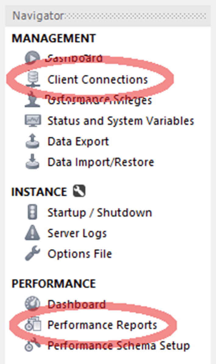
Accessing the client connections and performance reports
The rest of the section will discuss the two types of reports in more detail.
Performance Reports
The performance reports in MySQL Workbench are a great way to investigate what is happening in the instance. As the performance reports are based on the sys schema views, the information available will be the same as was discussed when going through the sys schema views.
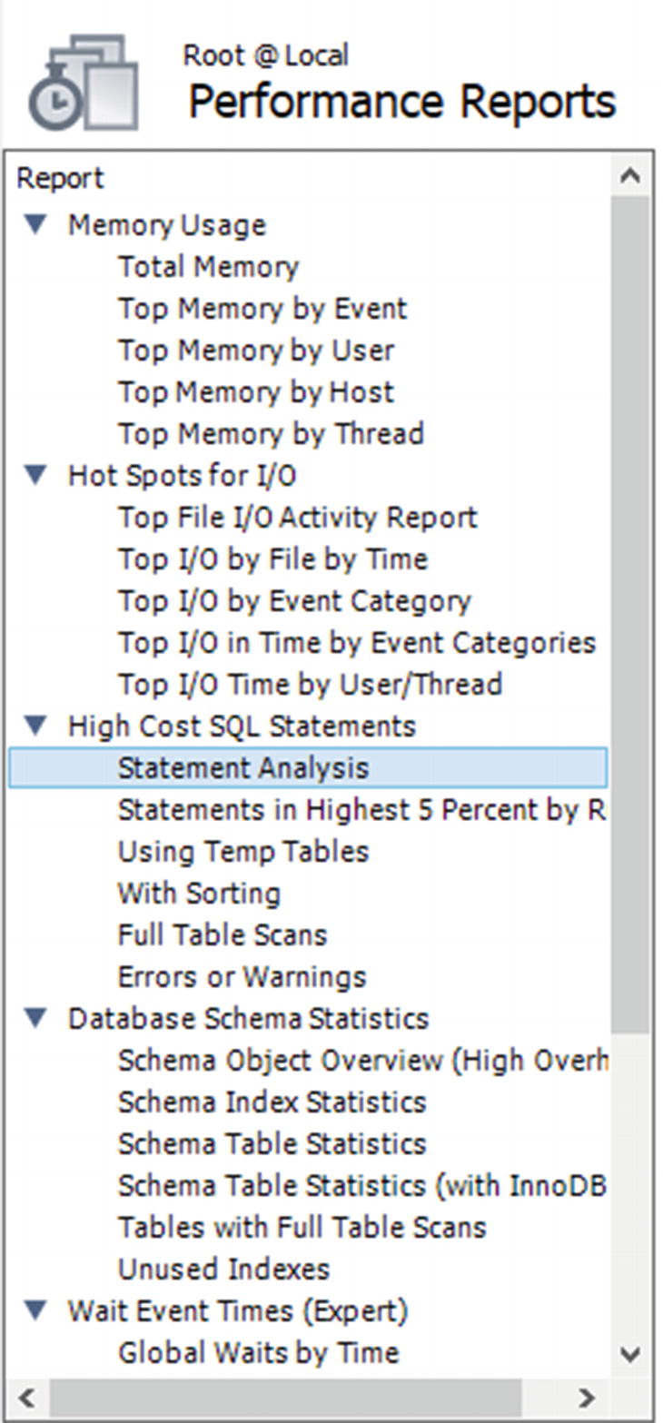
Choosing a performance report
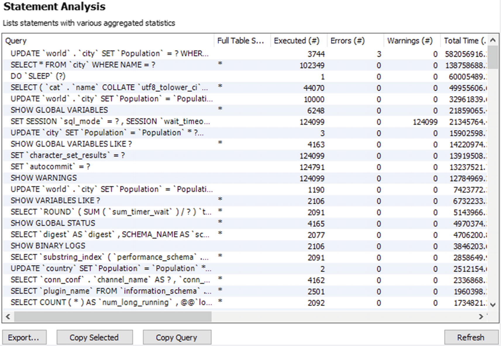
The statement statistics performance report
One advantage of the performance reports is that they use the unformatted view definitions, so you can change the ordering using the GUI. You change the ordering by clicking the column header for the column you want to order by. The order toggles between ascending and descending order each time you click the column header.
At the bottom of the report, there are buttons to help you use the report. The Export… button allows you to save the result of the report as a CSV file. The Copy Selected button copies the header and the selected rows into memory in the CSV format. The Copy Query button copies the query used for the report. This allows you to edit the query and manually execute it. For the report in Figure 19-3, the query returned is select ∗ from sys.`x$statement_analysis`. The final button is the Refresh button to the right which executes the report again.
There is no performance report based on the sys.session view. Instead you need to use the client connections report.
Client Connections Report
If you want to get a list of the connections currently connected to the instance, you need to use the client connections report. It does not include quite as much information as the sys.session view, but it does include the most essential data. The report is based on the threads table in the Performance Schema, and additionally, the program name is included if possible.
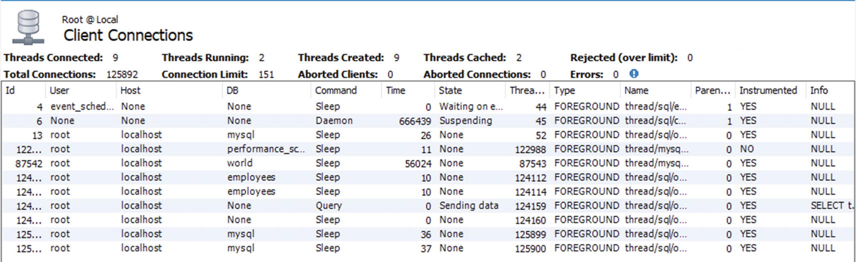
The client connections report
If you already have the client connections report or one of the performance reports open, you can reuse the connection to fetch the client connections report. That can be useful if all connections have been used up and you need to get a report of what the connections are doing. The client connections report also allows you to kill queries or connections by selecting the query and using one of the kill buttons to the lower right of the report.
While MySQL Workbench is very useful for investigating performance issues, it is primarily targeted at ad hoc investigations. For proper monitoring, you need a full monitoring solution.
MySQL Enterprise Monitor
There is not really anything replacing a full-featured monitoring solution when you need to investigate performance issues whether you are reacting to user complaints or are proactive looking to make improvements. This section will base the discussion on MySQL Enterprise Monitor (MEM). Other monitoring solutions may provide similar features.
There are three features that will be discussed in this section. The first is the Query Analyzer, then timeseries graphs, and finally ad hoc reports such as the processes and lock waits reports. You should use the various metrics in combination when you investigate an issue. For example, if you have a report of high disk I/O usage, then find the timeseries graphs showing disk I/O and determine how and when the I/O has developed. You can then use the Query Analyzer to investigate which queries were executed during this period. If the issue is still ongoing, a report like the processes report or one of the other ad hoc reports can be used to see what is going on.
The Query Analyzer
The Query Analyzer in MySQL Enterprise Monitor is one of the most important places to look when you need to investigate performance issues. MySQL Enterprise Monitor uses the events_statements_summary_by_digest table in the Performance Schema to regularly collect which queries have been executed. It then compares successive outputs to determine the statistics since the previous data collection. This is similar to what you saw in the example using the statement performance analyzer in the sys schema, just that this is happening automatically and is integrated together with the rest of the collected data.
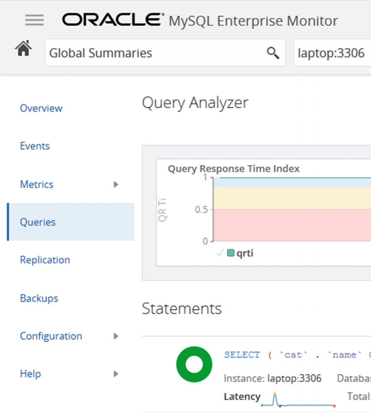
Accessing the Query Analyzer
Once you open the Query Analyzer, it will default to open with the Query Response Time index (QRTi) graph at the top and a list of queries below. The default time frame is the past hour. You can choose to display another graph or change the number of graphs. The default graph with the Query Response Time index is worth some consideration.
Optimum: When the query executes in less time than the threshold set to define optimal performance. The default threshold is 100 ms. The threshold can be configured. Green is used for the optimal time frame.
Acceptable: When the query executes in more time than the threshold for the optimal time frame but less than four times the threshold. This frame uses yellow.
Unacceptable: When the query is slower than four times the threshold for the optimal threshold. This frame uses red.
The Query Response Time index is not a perfect measure of how well the instance is performing, but for systems where the various queries are expected to have response times around the same interval, it does provide a good indication of how well the system or query performs at different times. If you have a mix of very fast OLTP queries and slow OLAP queries, it is not so good a measure of the performance.
If you spot something interesting in the graph, you can select that period and use that as the new time frame for filtering the queries. There is also the Configuration View button to the upper right of the graph that can be used to set the time frames for the graphs and queries, which graphs to show, filters for the queries, and so on.
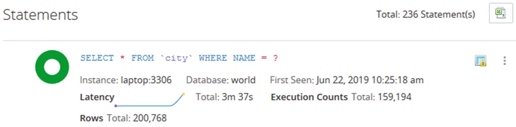
Overview of a query in the Query Analyzer
The information is high level and is meant to help you narrow down which candidate queries to look closer at for a given period. In the example, you can see that there have been almost 160,000 executions of the query to find cities by name. The first question you should ask is whether that is a reasonable amount of times to execute this query. It may be expected, but a high execution count may also be a sign of a runway process that keeps executing the same query over and over or that you need to implement caching for the query. You can also see from the green donut that all executions are in the optimal time frame with respect to the Query Response Time index.
The icon in the upper-right corner of the query area, just to the left of the three vertical dots, shows that MySQL Enterprise Monitor has flagged this query. To get the meaning of the icon, hover over the icon. The icon in this example means that the query is doing full table scans. Thus, even though the Query Response Time index looks good for the query, it is worth looking closer at the query. Whether it is acceptable that a full table scan is done depends on several factors such as the number of rows in the table and how often the query is executed. You can also see that the query latency graph shows an increase in latency at the right end of the graph suggesting the performance is degrading.
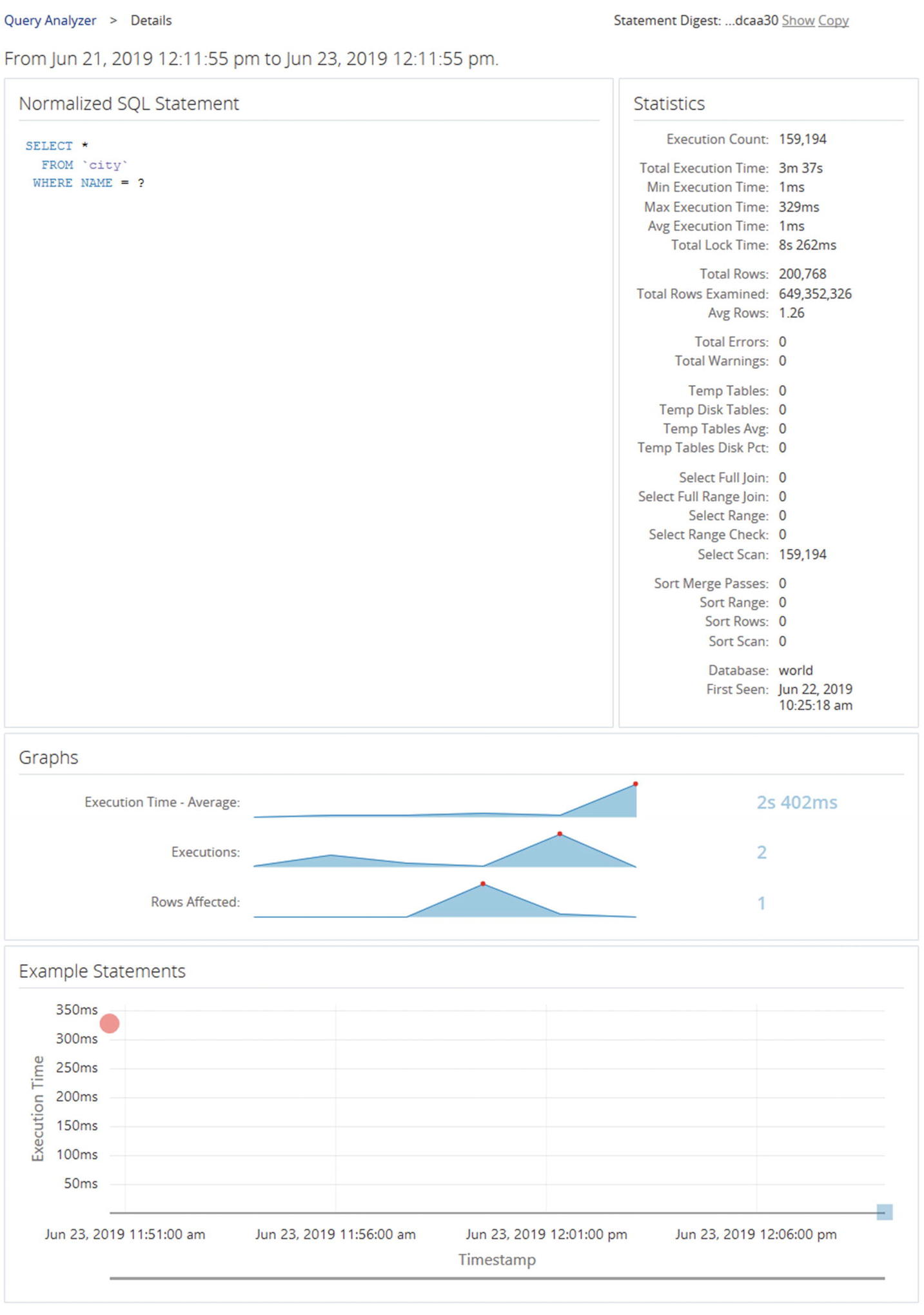
Query details from the Query Analyzer
The details include the metrics that are available from the Performance Schema digest summary. Here you can see that there are indeed much more rows examined than returned, so it is worth investigating further whether an index is required. The graphs give an idea of the development of the query execution over time.
At the bottom are examples of actual query execution latencies. In this case there are two executions included. The first is the red circle in the left of the graph. The second is the blue-greenish mark at the lower right. The color symbolized the Query Response Time index for each execution. This graph is only available if the events_statements_history_long consumer is enabled.
The Query Analyzer is great for investigating queries, but to get a higher-level summary of the activity, you need to use the timeseries graphs.
Timeseries Graphs
Timeseries graphs are what is often thought of when talking about a monitoring system. They are important to understand the overall load on the system and to spot changes over time. However, they are often not very good at finding the root cause of an issue. For that you need to analyze the queries or generate ad hoc reports to see the issue happening.
When you look at timeseries graphs, you need to consider a few things; otherwise, you may end up drawing the wrong conclusions and declare an emergency when there are no problems. First, you need to know what the metric in the graph means, like the discussion earlier in the chapter of what the I/O latencies mean. Second, remember that a change in the metric does not on its own mean there is a problem. It just means that the activity changed. If you start to execute more queries, because you enter the peak period of the day or year, it is only natural that the database activity increases and vice versa when you go to a quiet period. Similarly, if you implement a new feature such as adding an element to the start screen of the application, that is also expected to increase the amount of work performed. Third, be careful not just to consider a single graph. If you look at monitoring data without taking the other data into consideration, it is easy to make the wrong conclusions.
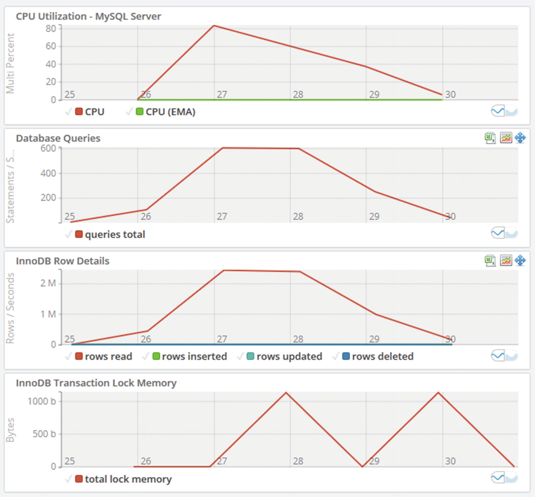
Timeseries graphs
If you look at the graphs, you can see the CPU utilization in the topmost graph suddenly increases and peaks at more than 80%. Why did that happen and is it a bad thing? The database queries graph shows that the number of statements per second increases at the same time and so does the number of rows read in the InnoDB row details graph. So the CPU usage is most likely caused by increased query activity. From there, you can go to the Query Analyzer and investigate which queries are running.
A couple of other points can be taken away from the graphs. If you look at the x-axis, the graph only covers six minutes of data. Be careful not to draw conclusions based on a very short time frame as that may not represent the true state of the system. The other thing is to remember to look at the scale of the data. Yes, the CPU usage and InnoDB transaction lock memory suddenly increase, but it happens from a base of 0. How many CPUs do the system have? If you have 96 CPUs, then using 80% of one CPU is really nothing, but if you are on a single CPU virtual machine, you have less headroom. For the transaction lock memory, if you take the y-axis into account, you can see that the “spike” is just 1 KiB of lock memory – so not something to worry about.
Sometimes you need to investigate an ongoing issue in which case the timeseries graphs and the Query Analyzer may not be able to give you the information you need. In that case you need ad hoc reports.
Ad Hoc Reports
There are several ad hoc reports available in MySQL Enterprise Monitor. Other monitoring solutions may have similar or other reports. The reports are similar to the information available from the sys schema reports that were discussed earlier in the chapter. One advantage of accessing ad hoc reports through the monitoring solution is that you can reuse the connections in case the application has used all connections available, and it provides a graphical user interface to manipulate the reports.
Table Statistics: This report shows how much each table is used based on the total latency, rows fetched, rows updated, and so on. It is equivalent to the schema_table_statistics view.
User Statistics: This report shows the activity for each username. It is equivalent to the user_summary view.
Memory Usage: This report shows the memory usage per memory type. It is equivalent to the memory_global_by_current_bytes view.
Database File I/O: This report shows the disk I/O usage. There are three options for the report: to group by file which is equivalent to the io_global_by_file_by_latency view, to group by the wait (I/O) type which is equivalent to the io_global_by_wait_by_latency view, and to group by thread which is equivalent to the io_by_thread_by_latency view. Grouping by the wait type adds the I/O-related timeseries graphs.
InnoDB Buffer Pool: This report shows what data is stored in the InnoDB buffer pool. It is based on the innodb_buffer_page Information Schema table. Since there can be a significant overhead querying the information for this report, it is recommended only to use the report on test systems.
Processes: This report shows the foreground and background threads that are currently present in MySQL. It uses the sys.processlist view which is the same as the session view except that it also includes background threads.
Lock Waits: This report has two options. You can either get a report for the InnoDB lock waits (the innodb_lock_waits view) or metadata locks (the schema_table_lock_waits view).
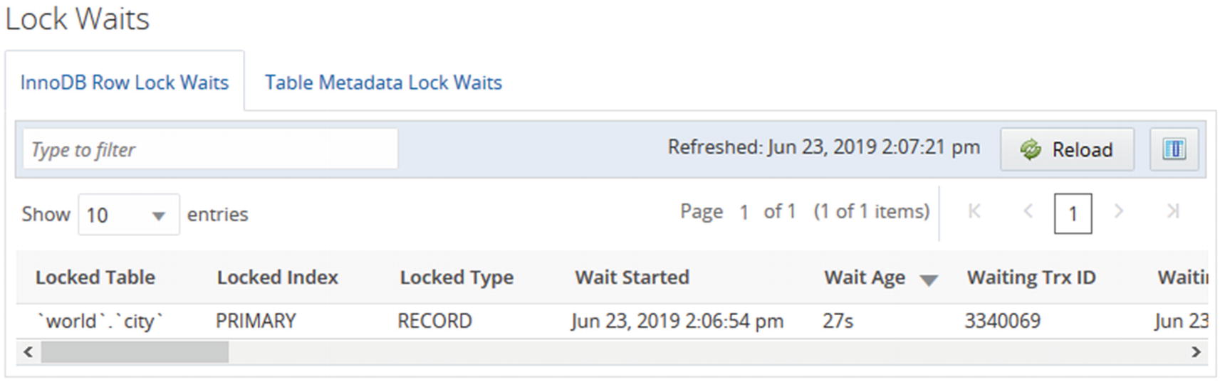
The InnoDB row lock waits report
The report shows the rows in a paginated mode, and you can change the ordering by clicking the column headers. Changing the ordering does not reload the data. If you need to reload the data, use the Reload button at the top of the screenshot.
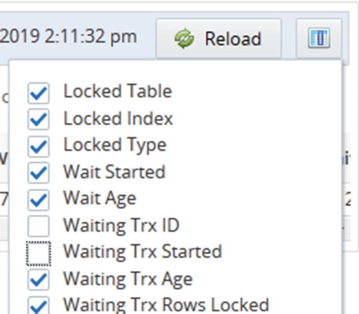
Choosing which columns to include in the report
When you toggle whether the columns are included or not, the report updates immediately without reloading the report. That means that for intermittent issues such as lock waits, you can manipulate the report without losing the data you are looking at. The same is the case if you change the ordering of the columns by dragging the column headers around.
Several of the reports have the choice between a standard column-based output and a treemap view. For the InnoDB buffer pool report, the treemap view is the only format supported. The treemap output uses rectangles with the area based on the value, so if a rectangle has twice the area of another rectangle, it means the value is twice as large. This can help visualize the data.
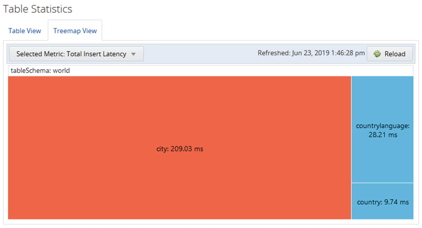
The treemap view of the total insert latency
When you look at the treemap view, you can immediately see that the amount of time spent on inserting data into the city table is much larger than for the other tables.
The ad hoc queries all deal with the state as it is at the time the report is executed. The Query Analyzer and timeseries graphs on the other hand work with what happened in the past. Another tool that shows what happened in the past is the slow query log.
The Slow Query Log
The slow query log is a trusty old tool for finding poorly performing queries and to investigate past problems in MySQL. It may seem unnecessary today where the Performance Schema has so many options to query statements that are slow, do not use indexes, or fulfill other criteria. However, the slow query log has one main advantage that it is persisted, so you can go back and use it even after MySQL has been restarted.
The slow query log is not enabled by default. You can enable and disable it using the slow_query_log option. The log can also be enabled and disabled dynamically without restarting MySQL.
There are two basic types of modes in which to use the slow query log. If you know when an issue occurred, you can check the log for slow queries at that time. One case is where queries have been piling up because of a lock issue, and you know when the issue ended. Then you can find that time in the log and look for the first query that completed with a long enough execution time to be part of the pileup issue; that query was likely the one causing the pileup possible in connection with some of the other queries finishing around or after that point in time.
The other usage mode is to use the mysqldumpslow utility to create an aggregate of the slow queries. This normalizes the queries similar to how the Performance Schema does, so similar queries will have their statistics aggregated. This mode is great to look for queries that may contribute to making the system busy.
You can choose what to sort the aggregated queries by with the -s option. You can use the total count (the c sorting value) to find the queries that are being executed the most. The more often a query is executed, the more benefit there is to optimize the query. You can use the total execution time (t) in a similar manner. If users are complaining about slow response times, the average execution time (at) is useful for sorting. If you suspect some queries return too many rows because they are missing filter conditions, you can sort the queries according to the number of rows they return (r for total rows, ar for average rows). Often it can be useful to combine the sorting option with the -r option to reverse the order and the -t to only include the first N queries. That way it is easier to focus on the queries causing the biggest impact.
You also need to remember that by default the slow query log does not log all queries, so you do not get the same insight into the workload as with the Performance Schema. You need to adjust the threshold for considering a query slow by changing the long_query_time configuration option. The option can be changed for a session, so if you have significant variations in expected execution time, you can set the global value to match the majority of queries and change per session for the connection executing queries that deviate from the normal. If you need to investigate issues that involve DDL statements, you need to make sure you enable the log_slow_admin_statements option.
The slow query log has a larger overhead than the Performance Schema. When just logging a few slow queries, the overhead is usually negligible, but it can be significant if you log many queries. Do not log all queries by setting long_query_time to 0 except on a test system or for a short period of time.
You analyze the mysqldumpslow reports in much the same way as the Performance Schema and sys schema, so it will be left as an exercise for the reader to generate reports from your systems and use them to find candidate queries for further optimization.
Summary
This chapter has explored the sources available to find queries that are candidates to be optimized. It was also discussed how to look for resource utilization that can be used to know at what times there are workloads that push the system most toward its limit. It is the queries running at that time that are the most important to focus on, though you should keep your eyes open for queries in general that do more work than they should.
The discussion started out going through the Performance Schema and considered which information is available and how to use it. Particularly the events_statements_summary_by_digest table is a gold mine when looking for queries that may have performance issues. You should however not restrict yourself to just looking at queries. You should also take table and file I/O into consideration as well as whether queries cause errors. These errors may include lock wait timeouts and deadlocks.
The sys schema provides a range of ready-made reports that you can use to find information. These reports are based on the Performance Schema, but they include filters, sorting, and formatting that make the reports easy to use, particularly as ad hoc reports when investigating an issue. It was also shown how the statement performance analyzer can be used to create a report of the queries running during a period of interest.
MySQL Workbench provides both performance reports based on the sys schema views and a client connections report based on the threads table in the Performance Schema. These features allow you to make ad hoc reports through a graphical user interface which makes it easy to change the ordering of the data and to navigate the reports.
Monitoring is one of the most important tools available to maintain a good health of your system and investigate performance problems. MySQL Enterprise Monitor was used as the base of the monitoring discussion. Particularly the Query Analyzer feature is very useful to determine which queries impact the system the most, but it should be used in conjunction with the timeseries graphs to understand the overall state of the system. You can also create ad hoc queries that can be used, for example, to investigate ongoing issues.
Finally, you should not forget the slow query log that has the advantage over the Performance Schema statement tables that it persists the recording of the slow queries. This makes it possible to investigate issues that happened before a restart. The slow query log also records the time when a query completed which is useful when a user reports that at some time the system was slow.
What do you do when you have found a query that you want to investigate further? The first step is to analyze it which will be discussed in the next chapter.